Light flavor asymmetry of nucleon sea

Abstract

The light flavor antiquark distributions of the nucleon sea are calculated in the effective chiral quark model and compared with experimental results. The contributions of the flavor-symmetric sea-quark distributions and the nuclear EMC effect are taken into account to obtain the ratio of Drell-Yan cross sections $\sigma^{\mathrm{pD}}/2\sigma^{\mathrm{pp}}$, which can match well with the results measured in the FermiLab E866/NuSea experiment. The calculated results also match the measured $\bar{d}(x)-\bar{u}(x)$ from different experiments, but unmatch the behavior of $\bar{d}(x)/\bar{u}(x)$ derived indirectly from the measurable quantity $\sigma^{\mathrm{pD}}/2\sigma^{\mathrm{pp}}$ by the FermiLab E866/NuSea Collaboration at large $x$. We suggest to measure again $\bar{d}(x)/\bar{u}(x)$ at large $x$ from precision experiments with careful experimental data treatment. We also propose an alternative procedure for experimental data treatment.

1 INTRODUCTION

The nucleon sea is an active issue in hadron physics because of its importance in understanding both the nucleon structure and properties of strong interaction. In the early days, it was usually assumed that the sea of the proton was flavor symmetric between $u\bar{u}$ and $d\bar{d}$ quark-antiquark pairs, i.e., $\bar{u}^{\mathrm{p}}(x)=\bar{d}^{\mathrm{p}}(x)$. However, this assumption was found to be unjustified by the observation of the Gottfried sum rule (GSR) gottfried1967 violation from a number of experiments pa1991 ; nmc1994 ; NA51 ; E8661998 ; pea98 ; E866 ; HERMES . There have been many studies related to theoretical explanations of these observations and the flavor asymmetry of the nucleon sea Rev .

The Gottfried sum gottfried1967 is defined as $S_{\mathrm{G}}=\int_{0}^{1}[F_{2}^{\mathrm{p}}(x)-F_{2}^{\mathrm{n}}(x)]{\mathrm{d}x/x}$, which, when expressed in terms of quark momentum distributions, takes the form

$$S_{\mathrm{G}} = \int_{0}^{1}[F_{2}^{\mathrm{p}}(x)-F_{2}^{\mathrm{n}}(x)]\frac{\mathrm{d}x}{x}$$ (1)

$$= \int_{0}^{1}\sum_{i}e_{i}^{2}[q_{i}^{\mathrm{p}}(x)+\bar{q}_{i}^{\mathrm{p}}(x)-q_{i}^{\mathrm{n}}(x)-\bar{q}_{i}^{\mathrm{n}}(x)]\mathrm{d}x,$$

where $x$ is the Bjorken variable, $F_{2}^{\mathrm{p}}(x)$ and $F_{2}^{\mathrm{n}}(x)$ are the proton and the neutron structure functions, $e_{i}$ is the charge of the quark of flavor $i$, and $q_{i}^{\mathrm{N}}$ ($\bar{q}_{i}^{\mathrm{N}}$, N=n,p) is the quark (antiquark) distribution of the nucleon. Decomposing the quark distribution into valance ($V$) and sea ($Q$ for quark and $A$ for antiquark) components, we get

$$\int_{0}^{1}q_{i}^{\mathrm{N}}(x)\mathrm{d}x=\int_{0}^{1}[V_{i}^{\mathrm{N}}(x)+Q_{i}^{\mathrm{N}}(x)]\mathrm{d}x,$$ (2)

$$\int_{0}^{1}\bar{q}_{i}^{\mathrm{N}}(x)dx=\int_{0}^{1}A_{i}^{\mathrm{N}}(x).$$ (3)

From the flavor number conservation and the isospin symmetry between the proton and the neutron, i.e., $u^{\mathrm{p}}(x)=d^{\mathrm{n}}(x)$, $\bar{u}^{\mathrm{p}}(x)=\bar{d}^{\mathrm{n}}(x)$, etc., we get

$$S_{\mathrm{G}}=\frac{1}{3}-\frac{2}{3}\int_{0}^{1}[\bar{d}^{\mathrm{p}}(x)-\bar{u}^{\mathrm{p}}(x)]\mathrm{d}x.$$ (4)

If the nucleon sea is flavor symmetric, one arrives at the GSR

$$S_{\mathrm{G}}=\frac{1}{3}.$$ (5)

The violation of the GSR was first observed by the New Muon Collaboration (NMC) pa1991 at CERN in 1991, and the reported Gottfried sum is $\int_{0}^{1}[F_{2}^{\mathrm{p}}(x)-F_{2}^{\mathrm{n}}(x)]{\mathrm{d}x/x}=0.240\pm 0.016$. In 1994 the NMC reanalyzed their data nmc1994 , and got $\int_{0}^{1}[F_{2}^{\mathrm{p}}(x)-F_{2}^{\mathrm{n}}(x)]{\mathrm{d}x/x}=0.235\pm 0.026$. Though the isospin symmetry breaking between the proton and the neutron at the parton level could also contribute m92 , at least partially, to the GSR violation, the results are usually interpreted as an indication of light flavor asymmetry of the nucleon sea Preparata:1990fd , and the excess of $d\bar{d}$ pairs over $u\bar{u}$ pairs in the nucleon sea was measured as nmc1994

$$\int_{0}^{1}[\bar{d}^{\mathrm{p}}(x)-\bar{u}^{\mathrm{p}}(x)]\mathrm{d}x=0.148\pm 0.039.$$ (6)

The Drell-Yan process Drell1971 can be used to measure the flavor distribution of the nucleon sea. The cross section of the Drell-Yan process at leading order is

$$\sigma^{\mathrm{AB}}\propto\sum_{i}e_{i}^{2}[q_{i}^{\mathrm{A}}(x_{1},Q^{2})\bar{q}_{i}^{\mathrm{B}}(x_{2},Q^{2})$$

$$+\bar{q}_{i}^{\mathrm{A}}(x_{1},Q^{2})q_{i}^{\mathrm{B}}(x_{2},Q^{2})],$$ (7)

where the sum is over all quark flavors, $e_{i}$ is the charge of the quark of flavor $i$, $q_{i}^{\mathrm{A}}~{}(\bar{q}_{i}^{\mathrm{A}})$ is the quark (antiquark) distribution of the beam, $q_{i}^{\mathrm{B}}~{}(\bar{q}_{i}^{\mathrm{B}})$ is the quark (antiquark) distribution of the target, and $x_{1}$ and $x_{2}$ are the Bjorken variables $x$ of the partons from the beam and the target respectively. Two kinematic quantities commonly used to describe Drell-Yan process are Feynman-$x$, $x_{\mathrm{F}}=x_{1}-x_{2}$, and the dilepton mass $M$, $M^{2}=Q^{2}\approx x_{1}x_{2}s$, where $Q^{2}$ and $\sqrt{s}$ are the square of the invariant momentum transferred and the center-of-mass energy of the initial nucleons respectively.

The FermiLab E772 Collaboration E772 reported an upper limit on the $\bar{d}$-$\bar{u}$ asymmetry in the range $0.04\leq x\leq 0.27$. Later, the CERN NA51 experiment NA51 measured the ratio of cross sections for muon pair production through the Drell-Yan process in $\mathrm{p}\mathrm{p}$ and $\mathrm{p}\mathrm{D}$ reactions at $y\sim 0$, with $450$ GeV/c incident protons. The Drell-Yan asymmetry is measured as $A_{\rm{DY}}=(\sigma^{\rm{pp}}-\sigma^{\rm{pn}})/(\sigma^{\rm{pp}}+\sigma^{\rm{pn}})=-0.09\pm 0.02\pm 0.025$. The ratio of $\bar{u}$ over $\bar{d}$ of the nucleon sea derived from this measurement is

$$\frac{\bar{u}^{\mathrm{p}}}{\bar{d}^{\mathrm{p}}}|_{<x>=0.18}=0.51\pm 0.04\pm 0.05.$$ (8)

However, the acceptance of NA51 spectrometer is peaked near $x_{\mathrm{F}}=0$ and $x=0.18$, and consequently we are almost impossible to determine the $x$-dependence of $\bar{d}^{\mathrm{p}}/\bar{u}^{\mathrm{p}}$ based on the NA51 experiment.

The FermiLab E866/NuSea Collaboration E866 measured the ratio of cross sections of Drell-Yan muon pairs from $800$ GeV/c proton beam scattered on liquid hydrogen and deuterium targets and extracted $\bar{d}(x)/\bar{u}(x)$ and $\bar{d}(x)-\bar{u}(x)$ in the proton sea over a wide range of $x$, and got $\int_{0}^{1}[\bar{d}(x)-\bar{u}(x)]\mathrm{d}x=0.118\pm 0.012$. However, the shape of $\bar{d}^{\mathrm{p}}(x)/\bar{u}^{\mathrm{p}}(x)$ is beyond expectation and the ratio can even be less than 1 when $x$ is large, which has received widespread attention because so large flavor asymmetry of $\bar{d}$ and $\bar{u}$ was unexpected and it is even more difficult to explain the result that $\bar{d}(x)<\bar{u}(x)$ when $x$ is large. The HERMES Collaboration HERMES measured charged hadrons from semi-inclusive deep-inelastic scattering, and reported $\bar{d}(x)-\bar{u}(x)$ over the range $0.02\leq x\leq 0.3$ and $1~{}\mathrm{GeV}^{2}/\mathrm{c}^{2}<Q^{2}<10~{}\mathrm{GeV}^{2}/\mathrm{c}^{2}$. Their result of $\bar{d}(x)-\bar{u}(x)$ is in agreement with that reported by the E866/NuSea experiment.

In 1977 Field and Feynman Field pointed out that $\bar{d}=\bar{u}$ would not strictly hold even in the perturbative Quantum Chromodynamics (QCD), due to the fact that an extra valance up quark in the proton can lead to a suppression of $g\rightarrow u\bar{u}$ relative to $g\rightarrow d\bar{d}$ via Pauli blocking. Nevertheless later calculations Ross ; Steffens indicated that the effects of Pauli blocking are very small and such large asymmetry must have a nonperturbative origin. The role of mesons in DIS was first investigated by Sullivan Sullivan . He suggested that some fraction of the sea antiquark distribution of the nucleon may be associated with the pion cloud around the nucleon core. This was the original idea of the meson cloud model. Many authors used the pion cloud mechanism Thom83 ; Kuma91 ; emh ; as ; js ; wyp or baryon-meson fluctuation picture Bo-Qiang Ma of the nucleon to explain the light flavor asymmetry of the nucleon sea. Besides, the effective chiral quark model Weinberg ; mg84 is also a method to explain the nucleon sea flavor asymmetry Eich92 ; wakamatsu and we discuss the details in Sec. 2. There are many other mechanisms to explain $\bar{d}\neq\bar{u}$, for example, chiral soliton model Pobylitsa , instanton model Dorokhov , statistical model statismodel and so on. But until now, no model can explain the $\bar{d}(x)/\bar{u}(x)<1$ behavior in the large $x$ region.

In Sec. 2, we use the effective chiral quark model Weinberg ; mg84 , with the constituent quark model hz81 and the light-cone quark-spectator-diquark model parton results respectively as the bare constituent quark distributions inputs, to calculate the quark distributions of the proton. From the isospin symmetry between the proton and the neutron, we obtain the quark distributions of the neutron. In Sec. 3, we take the symmetric quark and antiquark sea contribution and the $Q^{2}$-evolution of quark distribution into consideration, to obtain $\sigma^{\mathrm{pD}}/2\sigma^{\mathrm{pp}}$, $\bar{d}(x)-\bar{u}(x)$ and $\bar{d}(x)/\bar{u}(x)$. In Sec. 4, we discuss the possible nuclear EMC effect in the extraction of the ratio $\bar{d}(x)/\bar{u}(x)$. By taking into account such effect, the behavior of $\sigma^{\mathrm{pD}}/2\sigma^{\mathrm{pp}}$, which are really measured quantities rather than $\bar{d}(x)/\bar{u}(x)$, can match with the experimental results better when $x$ is large. Sec. 5 is devoted to some conclusions and summary.

2 THE SEA CONTENT IN THE EFFECTIVE CHIRAL QUARK MODEL

The effective chiral quark model, established by Weinberg Weinberg , and developed by Manohar and Georgi mg84 , has been widely recognized by the hadron physics society as an effective theory of QCD at the low energy scale. The effective chiral quark model has an apt description of its important degrees of freedom in terms of quarks, gluons and Goldstone (GS) bosons at momentum scales relating to hadron structure. There has been a prevailing impression that the effective chiral quark model is successful in explaining the violation of GSR from a microscopic viewpoint Eich92 ; wakamatsu . Also, this model plays an important role in explaining the proton spin crisis a89 in Refs. cl95 ; songxiaotong . A study by Ding and Xu with one of us dxm04 also shows that the strange-antistrange asymmetry within the effective chiral quark model could explain the NuTeV anomaly. We adopt the effective chiral quark model to calculate the quark and antiquark distributions of nucleons in this paper. The principles and basic formulas are almost the same as those used previously, but the options and inputs are carefully considered and some of them are differently chosen to make the results closer to the data.

The chiral symmetry at the high energy scale and its breaking at the low energy scale are the basic properties of QCD. Because the effect of the internal gluons is small in the effective chiral quark model at the low energy scale, the gluonic degrees of freedom are negligible when comparing to GS bosons and quarks. In this picture, the valence quarks contained in the nucleon fluctuate into quarks plus GS bosons, which spontaneously break chiral symmetry, and any low energy hadron properties should include this symmetry violation. The effective interaction Lagrangian is

$$L=\bar{\psi}(iD_{\mu}+V_{\mu})\gamma^{\mu}\psi+ig_{A}\bar{\psi}A_{\mu}\gamma^{\mu}\gamma_{5}\psi+\cdots,$$ (9)

where

$$\psi=\left(\begin{array}[]{c}u\\ d\\ s\\ \end{array}\right)$$ (10)

is the quark field and $D_{\mu}=\partial_{\mu}+igG_{\mu}$ is the gauge-covariant derivative of QCD, with $G_{\mu}$ standing for the gluon field, $g$ standing for the strong coupling constant and $g_{A}$ standing for the axial-vector coupling constant determined from the axial charge of the nucleon. $V_{\mu}$ and $A_{\mu}$ are the vector and the axial-vector currents which are defined by

$$\left(\begin{array}[]{c}V_{\mu}\\ A_{\mu}\\ \end{array}\right)=\frac{1}{2}(\xi^{+}\partial_{\mu}\xi\pm\xi\partial_{\mu}\xi^{+}),$$ (11)

where $\xi=\mathrm{exp}(i\Pi/f)$, and $\Pi$ has the form

$$\Pi\equiv\frac{1}{\sqrt{2}}\left(\begin{array}[]{ccc}\frac{\pi^{0}}{\sqrt{2}}+\frac{\eta}{\sqrt{6}}&\pi^{+}&K^{+}\\ \pi^{-}&-\frac{\pi^{0}}{\sqrt{2}}+\frac{\eta}{\sqrt{6}}&K^{0}\\ K^{-}&\overline{K^{0}}&\frac{-2\eta}{\sqrt{6}}\\ \end{array}\right).$$ (12)

With the expansions for $V_{\mu}$ and $A_{\mu}$ in powers of $\Pi/f$, it gives $V_{\mu}=0+O(\Pi/f)^{2}$ and $A_{\mu}=i\partial_{\mu}\Pi/f+O(\Pi/f)^{2}$, where the pseudoscalar decay constant is $f\simeq 93$ MeV. Thus, the effective interaction Lagrangian between GS bosons and quarks in the leading order becomes Eich92

$$L_{\Pi q}=-\frac{g_{A}}{f}\bar{\psi}\partial_{\mu}\Pi\gamma^{\mu}\gamma_{5}\psi.$$ (13)

We should point out that we use the perturbative expansion in the energy rather than in the effective couple constant, which can be large. Although this model contains an infinite number of terms, at a given order in the energy expansion, the low-energy theory is specified by a finite number of couplings. Therefore if the energy scale that we consider is low, the perturbative expansion is applicable regardless of the value of the coupling constant. The framework that we use in this paper is based on the time-ordered perturbative theory in the infinite momentum frame (IMF). Because all particles are on-mass-shell in this frame and the factorization of the subprocess is automatic, we neglect all possible off-mass-shell corrections. In this framework, we can express the quark distributions inside a nucleon as a convolution of a constituent quark distribution in a nucleon and the structure functions of a constituent quark. The light-front Fock decompositions of constituent quark wave functions have the following forms

$$|U\rangle=\sqrt{Z}|u_{0}\rangle+a_{\pi}|d\pi^{+}\rangle+\frac{a_{\pi}}{\sqrt{2}}|u\pi^{0}\rangle+a_{K}|sK^{+}\rangle+\frac{a_{\eta}}{\sqrt{6}}|u\eta\rangle,$$ (14)

$$|D\rangle=\sqrt{Z}|d_{0}\rangle+a_{\pi}|u\pi^{-}\rangle+\frac{a_{\pi}}{\sqrt{2}}|d\pi^{0}\rangle+a_{K}|sK^{0}\rangle+\frac{a_{\eta}}{\sqrt{6}}|d\eta\rangle.$$ (15)

Here, $Z$ is the renormalization constant for the bare constituent quarks which are massive and denoted by $|u_{0}\rangle$ and $|d_{0}\rangle$, and $|a_{\alpha}|^{2}$ are the probabilities to find GS bosons in the dressed constituent quark states ($|U\rangle$ for an $up$ quark and $|D\rangle$ for a $down$ quark), where $\alpha=\pi,K,\eta$. In the effective chiral quark model, the fluctuation of a bare constituent quark into a GS boson and a recoil bare constituent quark can be given as sw98

$$q_{j}(x)=\int^{1}_{x}\frac{\textmd{d}y}{y}P_{j\alpha/i}(y)q_{i}\left(\frac{x}{y}\right).$$ (16)

In Eq. (16), $P_{j\alpha/i}(y)$ is the splitting function for the probability to find a constituent quark $j$ carrying the light-cone momentum fraction $y$ together with a spectator GS boson $\alpha$, and it has the following form

$$P_{j\alpha/i}(y) = \frac{1}{8\pi^{2}}\left(\frac{g_{A}\overline{m}}{f}\right)^{2}$$ (17)

$$\times \int\textmd{d}k^{2}_{T}\frac{(m_{j}-m_{i}y)^{2}+k^{2}_{T}}{y^{2}(1-y)[m_{i}^{2}-M^{2}_{j\alpha}]^{2}},$$

where $m_{i},m_{j},m_{\alpha}$ are the masses of the $i$-, $j$-constituent quarks and the pseudoscalar meson $\alpha$, respectively, $\overline{m}=(m_{i}+m_{j})/2$ is the average mass of constituent quarks, and $M_{j\alpha}^{2}$ is the square of the invariant mass of the final states,

$$M^{2}_{j\alpha}=\frac{m^{2}_{j}+k^{2}_{T}}{y}+\frac{m^{2}_{\alpha}+k^{2}_{T}}{1-y}.$$ (18)

In this paper, we adopt the definition of the moment of the splitting function

$$\langle x^{n-1}P_{j\alpha/i}\rangle=\int^{1}_{0}x^{n-1}P_{j\alpha/i}(x)\textmd{d}x$$ (19)

with the first moment $\langle P_{j\alpha/i}\rangle=\langle P_{\alpha j/i}\rangle\equiv\langle P_{\alpha}\rangle=|a_{\alpha}|^{2}$ sw98 . In terms of the above notation, the renormalization constant $Z$ is given by

$$Z=1-\frac{3}{2}\langle P_{\pi}\rangle-\langle P_{K}\rangle-\frac{1}{6}\langle P_{\eta}\rangle.$$ (20)

Now we need to specify the momentum cutoff function at the quark-GS boson vertex. It is conventional to use an exponential cutoff in IMF calculations,

$$g_{A}\rightarrow g_{A}^{\prime}\textmd{exp}\bigg{[}\frac{m^{2}_{i}-M^{2}_{j\alpha}}{4\Lambda^{2}}\bigg{]},$$ (21)

with $g_{A}^{\prime}=1$ following the large $N_{c}$ argument w90 . However, $g_{A}^{\prime}=0.75$ was adopted in the original work mg84 . Such a form factor has the correct $t$ and $u$ channel symmetry, and $\Lambda$ is the cutoff parameter, which is determined by the experimental data of the Gottfried sum and the constituent quark mass inputs for the pion. This function satisfies the symmetry $P_{j\alpha/i}(y)=P_{\alpha j/i}(1-y)$.

When probing the internal structure of GS bosons, we can write the process in the following form sw98

$$q_{k}(x)=\int\frac{\textmd{d}y_{1}}{y_{1}}\frac{\textmd{d}y_{2}}{y_{2}}V_{k/\alpha}\left(\frac{x}{y_{1}}\right)P_{\alpha j/i}\left(\frac{y_{1}}{y_{2}}\right)q_{i}\left(y_{2}\right),$$ (22)

where $V_{k/\alpha}(x)$ is the quark $k$ distribution function in $\alpha$ and satisfies the normalization $\int_{0}^{1}V_{k/\alpha}(x)dx=1$. Because the mass of $\eta$ is so high and the coefficient is so small that the fluctuation of it is suppressed, the contribution of $\eta$ is not considered in our calculation. From Eqs. (14) and (15), we obtain the quark distribution functions of nucleon by using the splitting function Eq. (17) and the constituent quark distributions $u_{0}$ and $d_{0}$,

$$u(x) = Zu_{0}(x)+P_{u\pi^{-}/d}\otimes d_{0}+V_{u/\pi^{+}}\otimes P_{\pi^{+}d/u}\otimes u_{0}$$

$$+ \frac{1}{2}P_{u\pi^{0}/u}\otimes u_{0}+V_{u/K^{+}}\otimes P_{K^{+}s/u}\otimes u_{0}$$

$$+ \frac{1}{2}V_{u/\pi^{0}}\otimes(P_{\pi^{0}u/u}\otimes u_{0}+P_{\pi^{0}d/d}\otimes d_{0}),$$

$$d(x) = Zd_{0}(x)+P_{d\pi^{+}/u}\otimes u_{0}+V_{d/\pi^{-}}\otimes P_{\pi^{-}u/d}\otimes d_{0}$$ (23)

$$+ \frac{1}{2}P_{d\pi^{0}/d}\otimes d_{0}+V_{d/K^{0}}\otimes P_{K^{0}s/d}\otimes d_{0}$$

$$+ \frac{1}{2}V_{d/\pi^{0}}\otimes(P_{\pi^{0}u/u}\otimes u_{0}+P_{\pi^{0}d/d}\otimes d_{0}).~{}$$

Here, we define the notations for the convolution integral as

$$P_{j\alpha/i}\otimes q_{i}=\int_{x}^{1}\frac{\textmd{d}y}{y}P_{j\alpha/i}\left(y\right)q_{i}\left(\frac{x}{y}\right),$$ (24)

and

$$V_{k/\alpha} \otimes P_{\alpha j/i}\otimes q_{i}=$$

$$\int_{x}^{1} \frac{\textmd{d}y_{1}}{y_{1}} \int_{y_{1}}^{1}\frac{\textmd{d}y_{2}}{y_{2}}V_{k/\alpha}\left(\frac{x}{y_{1}}\right)P_{\alpha j/i}\left(\frac{y_{1}}{y_{2}}\right)q_{i}\left(y_{2}\right).$$ (25)

In the same way, we can derive the light-flavor antiquark distributions,

$$\bar{u}(x) = V_{\bar{u}/\pi^{-}}\otimes P_{\pi^{-}u/d}\otimes d_{0}$$

$$+ \frac{1}{2}V_{\bar{u}/\pi^{0}}\otimes(P_{\pi^{0}u/u}\otimes u_{0}+P_{\pi^{0}d/d}\otimes d_{0}),$$

$$\bar{d}(x) = V_{\bar{d}/\pi^{+}}\otimes P_{\pi^{+}d/u}\otimes u_{0}$$

$$+ \frac{1}{2}V_{\bar{d}/\pi^{0}}\otimes(P_{\pi^{0}u/u}\otimes u_{0}+P_{\pi^{0}d/d}\otimes d_{0}),$$

where

$$~{}~{}~{}V_{u/\pi^{+}}=V_{\bar{d}/\pi^{+}}=V_{d/\pi^{-}}=V_{\bar{u}/\pi^{-}}$$

$$=2V_{u/\pi^{0}}=2V_{\bar{u}/\pi^{0}}=2V_{d/\pi^{0}}=2V_{\bar{d}/\pi^{0}}$$

$$=\frac{1}{2}V_{\pi}\left(x\right),$$ (27)

and

$$V_{u/K^{+}}=V_{d/K^{0}}.$$

From above equations, we can reexamine the valence quark distributions $u_{v}(x)=u(x)-\bar{u}(x)$ and $d_{v}(x)=d(x)-\bar{d}(x)$, which satisfy the correct normalization with the renormalization constant $Z$. We should point out that in the chiral quark model, antiquarks are produced in the process of the splitting of Goldstone bosons unless higher order effects are considered. Since Goldstone bosons are spin-0 particles without polarization, antiquarks are unpolarized, and this feature is compatible with the available experimental data Hermes .

In this paper, we choose $m_{u}=m_{d}=330$ MeV, $m_{s}=480$ MeV, $m_{\pi^{\pm}}=m_{\pi^{0}}=140$ MeV and $m_{K^{+}}=m_{K^{0}}=495$ MeV. Employing the quark distributions of the effective chiral quark model, we get the Gottfried sum determined by the difference between the proton and the neutron structure functions,

$$S_{G} = \int^{1}_{0}\frac{\mathrm{d}x}{x}[F^{p}_{2}(x)-F^{n}_{2}(x)]$$ (28)

$$= \frac{1}{3}\int_{0}^{1}\mathrm{d}x[u(x)+\bar{u}(x)-d(x)-\bar{d}(x)]$$

$$= \frac{1}{3}(Z-\frac{1}{2}\left<P_{\pi}\right>+\left<P_{K}\right>+\frac{1}{6}\left<P_{\eta}\right>)$$

$$= \frac{1}{3}(1-2\left<P_{\pi}\right>).$$

From the above equation and the experimental value of Gottfried sum nmc1994 , we can find that the appropriate value for $\Lambda_{\pi}$ is $1500$ MeV. At the same time, $\langle P_{\pi}\rangle=0.149$, $\langle P_{K}\rangle=0.085$, $\langle P_{\eta}\rangle=0.063$ and $Z=0.682$. But for $K$ and $\eta$ mesons, the terms $\langle P_{K}\rangle$ and $\langle P_{\eta}\rangle$ in the Gottfried sum cancel out those terms in $Z=1-\frac{3}{2}\langle P_{\pi}\rangle-\langle P_{K}\rangle-\frac{1}{6}\langle P_{\eta}\rangle$, so the value of $\Lambda$ can not be determined from Eq. (28) or experimental data. It is natural to assume that the cutoffs are same for $\pi$, $K$ and $\eta$ mesons in the effective chiral quark model, $\Lambda_{\pi}=\Lambda_{K}=1500$ MeV sw98 ; Szcz96 , which is different from the traditional meson cloud model.

In this paper, the parton distributions for mesons are taken from the parametrization from GRS98 given by Gluck-Reya-Stratmann grs98 because the results from parametrization can be closer to reality than those from models,

$$V_{\pi}(x)=0.942x^{-0.501}(1+0.632\sqrt{x})(1-x)^{0.367},$$

$$V_{u/K^{+}}(x)=V_{d/K^{0}}(x)=0.541(1-x)^{0.17}V_{\pi}(x).$$ (29)

We also need inputs of constituent-quark distributions $u_{0}$ and $d_{0}$. But there is no proper parametrization of them because they cannot be directly measured in the experiment. Therefore, we have to choose some models as inputs. In this paper the constituent quark model distributions hz81 and the light-cone quark-spectator-diquark model distributions parton are adopted as two different kinds of inputs of constituent quark distributions. The constituent quark model distributions have the following forms

$$u_{0}(x) = \frac{2}{\textmd{B}[c_{1}+1,c_{1}+c_{2}+2]}x^{c_{1}}(1-x)^{c_{1}+c_{2}+1},$$

$$d_{0}(x) = \frac{1}{\textmd{B}[c_{2}+1,2c_{1}+2]}x^{c_{2}}(1-x)^{2c_{1}+1},$$ (30)

where $B[i,j]$ is the Euler beta function, and $c_{1}=0.65$ and $c_{2}=0.35$ adopted from Ref. hz81 ; kko99 can satisfy the number sum rules

$$\int^{1}_{0}u_{0}(x)\textmd{d}x=2,~{}~{}~{}~{}\int^{1}_{0}d_{0}(x)\textmd{d}x=1,$$ (31)

and the momentum sum rule

$$\int_{0}^{1}xu_{0}(x)\textmd{d}x+\int_{0}^{1}xd_{0}(x)\textmd{d}x=1.$$ (32)

It is pointed out that there are other different values for $c_{1}$ and $c_{2}$ suggested by Ref. hy02 . The light-cone quark-spectator-diquark model distributions parton are

$$u_{0}(x) = \frac{1}{2}a_{S}(x)+\frac{1}{6}a_{V}(x),~{}~{}$$

$$d_{0}(x) = \frac{1}{3}a_{V}(x).~{}~{}$$ (33)

where $a_{D}(x)\propto\int[{\rm d}^{2}{\bf k}_{\perp}]|\varphi_{D}(x,{\bf k}_{\perp})|^{2}$ ($D=S$ or $V$) is normalized such that $\int_{0}^{1}dxa_{D}(x)=3$ and denotes the amplitude for the quark $q$ being scattered while the spectator is in the diquark state $D$. We adopt the Brodsky-Huang-Lepage prescription BHL for the light-cone momentum space wave function of the quark-spectator-diquark

$$\varphi_{D}(x,{\bf k}_{\perp})=A_{D}\exp\{-\frac{1}{8\beta^{2}_{D}}[\frac{m^{2}_{q}+{\bf k}^{2}_{\perp}}{x}+\frac{m^{2}_{D}+{\bf k}^{2}_{\perp}}{1-x}]\}.$$ (34)

where ${\bf k}_{\perp}$ is the internal quark transversal momentum, $m_{q}$ and $m_{D}$ are the masses of the quark $q$ and spectator $D$, and $\beta_{D}$ is the harmonic oscillator scale parameter. In this paper we simply adopt $m_{q}=330$ MeV, $\beta_{D}=330$ MeV, $m_{S}=600$ MeV and $m_{V}=800$ MeV as often adopted in literature. In the light-cone quark-spectator-diquark model, the number sum rule Eq. (31) is still satisfied but the momentum sum rule Eq. (32) is violated. It should be noticed that in this paper we adopt the quark-spectator-diquark model, i.e., when any quark is probed, the other part of the target is served as a spectator with quantum numbers of a diquark. Thus, some gluon effects may exist inside the spectators. This means that partial momentum can be carried by gluons at the initial point within the quark-spectator-diquark model. Hence there is no need to require the momentum sum rule Eq. (32) by quarks as in the constituent quark model, where the nucleon momentum is distributed among constituent quarks at the initial point.

3 ADDITIONAL SYMMETRIC SEA CONTRIBUTIONS

As is well-known, the quark distributions measured by experiments at certain $Q^{2}$ include not only non-perturbative intrinsic sea but also perturbative extrinsic sea Bo-Qiang Ma . Although the antiquark content in the nucleon mainly comes from the intrinsic sea, the extrinsic sea should also be considered from a strict sense when we want to investigate the distributions of quarks and antiquarks. Therefore, we take into account additional contribution from the symmetric sea before we use our quark distributions to compare with experimental data.

We should point out that the quark distribution functions we obtain in the front can only be proper at a certain $Q_{0}^{2}$, because the values of parameters in the model do not evolve according to $Q^{2}$. In the experiment of the E866/NuSea Collaboration, $Q^{2}$ varies from about $21$ GeV${}^{2}/$c² to more than $160$ GeV${}^{2}/$c², so the change of $Q^{2}$ should be considered carefully. In this paper, we choose $Q_{0}=0.7~{}$GeV/c. For simplicity, we also assume that the quark distribution functions we get have the same evolution behavior with that of parametrization we adopt,

$$q\left(x,Q^{2}\right)=q\left(x,Q_{0}^{2}\right)\frac{q^{\mathrm{para}}\left(x,Q^{2}\right)}{q^{\mathrm{para}}\left(x,Q_{0}^{2}\right)},$$ (35)

where $q=u$, $d$, $\bar{u}$, $\bar{d}$. The $q^{\mathrm{para}}$ stands for the quark distribution of flavor $q$ from parametrization.

It is found that most parametrizations of parton distributions after the experiment of E866/NuSea Collaboration had been considerably affected by it, so we adopt an earlier parametrization, namely CTEQ4 parametrization cteq4 . In this paper we will use $\bar{u}$ as the criterion. Other methods to take the contribution of symmetric sea may also work, and our method is a feasible choice. As we can see, the $\bar{u}(x)$ we derived from the model can be larger than that of CTEQ4 parameterization when $x$ is large, so we should not add symmetric sea contribution to $\bar{u}$ and $\bar{d}$ any more when they are larger than the result from parameterization. Specifically, if $\bar{u}^{\mathrm{model}}(x)<\bar{u}^{\mathrm{para}}(x)$, we estimate the symmetric sea contribution $\delta\bar{u}(x)=\delta\bar{d}(x)=\delta u(x)=\delta d(x)=\bar{u}^{\mathrm{para}}(x)-\bar{u}^{\mathrm{model}}(x)$, otherwise we set the symmetric sea to be zero. Intuitively, the flavor symmetric sea perturbative extrinsic can be thought as arising from the splitting of gluons to quark-antiquark pairs, thus they are flavor symmetric. Similar consideration has also been adopted to confront the calculated strange and antistrange distributions with experimental observations in the calculation of the strange-antistrange asymmetry in the chiral quark model dxm04 .

We compare the parton distributions derived above with the CTEQ4 parametrization and find that $\bar{u}$ and $\bar{d}$ quark distributions can match well while that $u$ and $d$ quark distributions really vary. Thus, we will adopt two methods to compare results with experimental data in the following: (1) we use parton distributions of both quarks and antiquarks from the model in the calculation, and this is denoted as “Model”; (2) we use parton distributions of $\bar{u}$ and $\bar{d}$ from the model while the distributions of $u$ and $d$ are parametrization results from CTEQ4 directly, and this is denoted as “Q.Para.”.

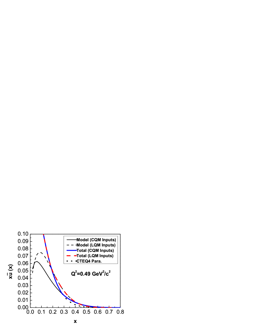
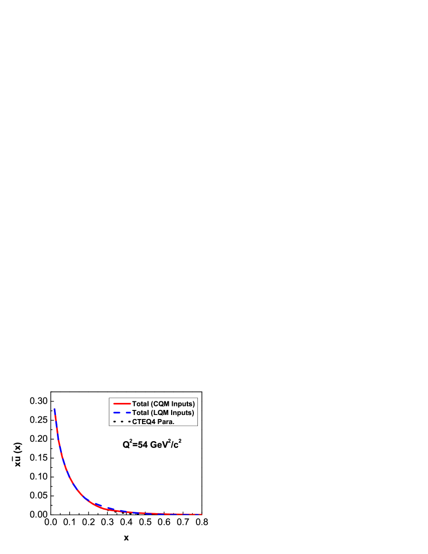
Figure 1: Distributions for $x\bar{u}(x)$, with $Q^{2}=0.49~{}\mathrm{GeV}^{2}/\mathrm{c}^{2}$ for the left part and $Q^{2}=54~{}\mathrm{GeV}^{2}/\mathrm{c}^{2}$ for the right part. The dotted curve is the result from CTEQ4 parametrization. The thin solid and dashed curves are the model calculation results with the constituent quark model (CQM) and the light-cone quark-spectator-diquark model (LQM) as inputs. The thick corresponding curves are the corresponding results with chiral quark model results plus the symmetric sea contributions.

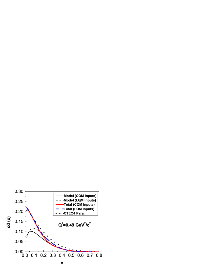
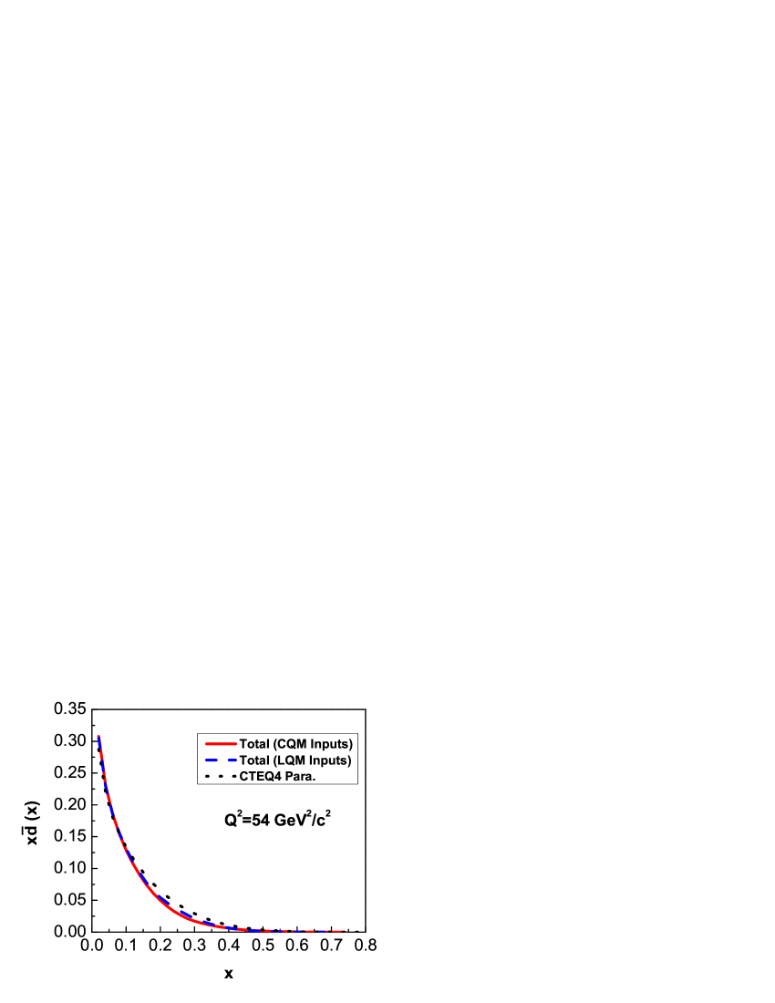
Figure 2: Distributions for $x\bar{d}(x)$, with $Q^{2}=0.49~{}\mathrm{GeV}^{2}/\mathrm{c}^{2}$ for the left part and $Q^{2}=54~{}\mathrm{GeV}^{2}/\mathrm{c}^{2}$ for the right part. The dotted curve is the result from CTEQ4 parametrization. The thin solid and dashed curves are the model calculation results with the constituent quark model (CQM) and the light-cone quark-spectator-diquark model (LQM) as inputs. The thick corresponding curves are the corresponding results with chiral quark model results plus the symmetric sea contributions.

The forms of cross sections we take are

$$\sigma^{\mathrm{pp}} \propto \frac{4}{9}u(x_{1})\bar{u}(x_{2})+\frac{1}{9}d(x_{1})\bar{d}(x_{2})$$ (36)

$$+ \frac{4}{9}\bar{u}(x_{1})u(x_{2})+\frac{1}{9}\bar{d}(x_{1})d(x_{2}),$$

and

$$\sigma^{\mathrm{pn}} \propto \frac{4}{9}u(x_{1})\bar{d}(x_{2})+\frac{1}{9}d(x_{1})\bar{u}(x_{2})$$ (37)

$$+ \frac{4}{9}\bar{u}(x_{1})d(x_{2})+\frac{1}{9}\bar{d}(x_{1})u(x_{2}).$$

The influence of heavier quarks is not included as their contributions can be reasonably neglected. With all these taken into consideration, we can get the results shown in Fig. 3 and Fig. 4. We find the results are quite good except when $x$ is large, regardless of the constituent quark distribution inputs and the methods we adopt. Accordingly, the approach taken by us should be reasonable.

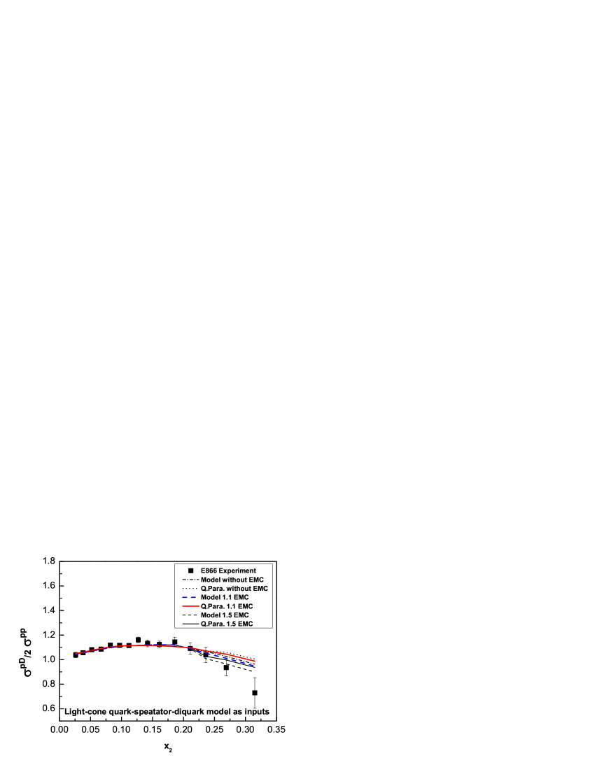
Figure 3: The Drell-Yan cross section ratio $\sigma^{\mathrm{pD}}/2\sigma^{\mathrm{pp}}$ versus $x_{2}$. The data are taken from E866/NuSea E866 experiment. The following curves are results from model with the light-cone quark-spectator-diquark model (LQM) as inputs plus symmetric sea contributions. The thin dash-dotted (dotted) curve is the result that the quark distribution from the chiral quark model (CTEQ4 parametrization) without EMC effect. The thick dashed (solid) curve is the corresponding result with EMC effect for the parameter $\xi=1.1$. The thin dashed (solid) curve is the corresponding result with EMC effect for the parameter $\xi=1.5$.

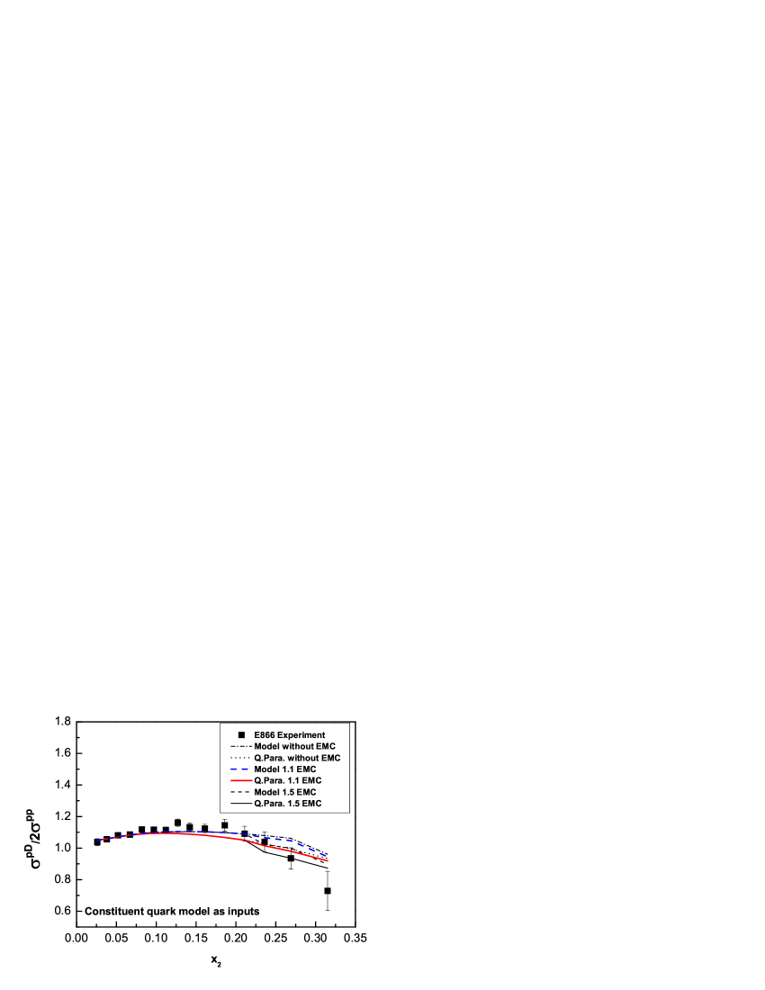
Figure 4: The Drell-Yan cross section ratio $\sigma^{\mathrm{pD}}/2\sigma^{\mathrm{pp}}$ versus $x_{2}$. The data are taken from E866/NuSea E866 experiment. The following curves are results from model with the constituent quark model (CQM) as inputs plus symmetric sea contributions. The thin dash-dotted (dotted) curve is the result that the quark distribution from the chiral quark model (CTEQ4 parametrization) without EMC effect. The thick dashed (solid) curve is the corresponding result with EMC effect for the parameter $\xi=1.1$. The thin dashed (solid) curve is the corresponding result with EMC effect for the parameter $\xi=1.5$.

4 DISCUSSION ON NUCLEAR EMC EFFECT

In 1982, the European Muon Collaboration (EMC) at CERN EMCA ; EMC found that the structure-function ratio of bound nucleon to free nucleon, in the form of $F^{\mathrm{A}}_{2}(x,Q^{2})/\\ F^{\mathrm{D}}_{2}(x,Q^{2})$, is not consistent with the expectation by assuming that a nuclei is composed by almost free nucleons with Fermi motion correction taken into account, and such phenomenon was confirmed by E139 collaboration at SLAC SLAC . This discovery, which is called the nuclear EMC effect, has received extensive attention by the nuclear and hadronic physics society. There are many models describing EMC effect now LEST ; ME ; Jaffe ; Carlson ; Vary ; FEC ; RLJ ; FECB ; ONachtmann , and a good review can be found in Ref. BLMA . All these models can qualitatively describe the data in the mediate $x$ region. The inclusive deep inelastic scattering (DIS) data are expressed as $F^{\mathrm{A}}_{2}(x,Q^{2})/F^{\mathrm{D}}_{2}(x,Q^{2})$, which can be written in the naive parton model as

$$\frac{F^{\mathrm{A}}_{2}(x,Q^{2})}{F^{\mathrm{D}}_{2}(x,Q^{2})}=\frac{\Sigma_{i}{e_{i}^{2}\left[q_{i}(x,Q^{2},\mathrm{A})+\bar{q}_{i}(x,Q^{2},\mathrm{A})\right]}}{\Sigma_{i}{e_{i}^{2}\left[q_{i}(x,Q^{2})+\bar{q}_{i}(x,Q^{2})\right]}},$$ (38)

where $e_{i}$ denotes the charge of the partons with flavor $i$, and $q(x,Q^{2})$ is the parton distribution function of the nucleon.

In the analysis of the E866/NuSea Collaboration, the nuclear effects in deuterium were assumed to be negligible. As discussed above, the calculated results of $\sigma^{\mathrm{pD}}/2\sigma^{\mathrm{pp}}$ cannot describe the experimental data well when $x$ is large, and this is just the region where the nuclear EMC effect may begin to work. So we will take the EMC effect into account to check how the results can be changed. In this paper, we choose the so-called $Q^{2}$-rescaling model Jaffe ; FECB ; FEC ; RLJ . In this model, the quark of a bound nucleon in the nuclear medium is considered to have different confinement size compared with that of the quark in the free nucleon, and consequently $q^{\mathrm{A}}(x,Q^{2})$ is related with $q^{\mathrm{N}}(x,Q^{2})$ (the parton distribution in the free nucleon) by the relation

$$q^{\mathrm{A}}\left(x,Q^{2}\right)=q^{\mathrm{N}}\left(x,\xi\left(Q^{2}\right)Q^{2}\right).$$ (39)

At $Q\approx 12.5$ GeV/c, we adopt $\xi=1.1$ given in the original work FECB . We show the ratio of $F_{2}^{\mathrm{D}}(x)$ in deuterium and that in a free proton plus a free neutron (denoted as p+n) in FIG.5. We assume furthermore that the nuclear EMC effect only takes effect when $x>0.22$. To show the dependence of the rescaling factor $\xi$, we also adopt a larger value $\xi=1.5$ as a comparison. Then we can see that the behavior of cross section ratio at large $x$ is visibly improved. In addition, we find that the cross section ratio at $\langle x_{2}\rangle=0.315$ is smaller than 1. We also display $\bar{d}(x)-\bar{u}(x)$ and $\bar{d}(x)/\bar{u}(x)$ in Fig.6 and Fig.7 respectively. As we can see, the behavior of $\bar{d}(x)-\bar{u}(x)$ we derived can match well with the experimental data and parametrization from CTEQ4, however, $\bar{d}(x)/\bar{u}(x)$ we get can match with experiment at small $x$ but is not compatible with the experiment at large $x$, and especially we could not get the ratio smaller than 1 in the region we consider. It is worthy to remind that all known models have the result that $\bar{d}(x)/\bar{u}(x)$ is larger than 1 over all $x$ range.

It is found that we can adopt an alternative procedure to deal with $u$ quark and $d$ quark to compare the result with the experiment. We assume $u(x)=u^{\mathrm{para}}(x)$ and $d(x)=d_{v}(x)+\bar{d}(x)$, where $d_{v}=d^{\mathrm{para}}-{\bar{d}}^{\mathrm{para}}$ is the valance $d$ quark distribution, and $\bar{d}$ is the result we get from the chiral quark model with symmetric sea quark distribution added. The result is denoted as “$\mathrm{D}_{\mathrm{v}}.\mathrm{Para}.$” and displayed in Fig. 8. We find that this result can also match well with the experimental data.

So we suggest a procedure for experimental data treatment to derive $\bar{d}(x)/\bar{u}(x)$ and $\bar{d}(x)-\bar{u}(x)$ from the cross section ratio $\sigma^{\mathrm{pD}}/2\sigma^{\mathrm{pp}}$: first assume $u(x)=u^{\mathrm{para}}(x)$, $\bar{u}(x)={\bar{u}}^{\mathrm{para}}(x)$ and $d(x)=d^{\mathrm{para}}(x)-{\bar{d}}^{\mathrm{para}}(x)+\bar{d}(x)$, then the experimental data is used to fit the behavior of $\bar{d}(x)$. This procedure might give results more compatible with model predictions than the method adopted in the E866/NuSea analysis.

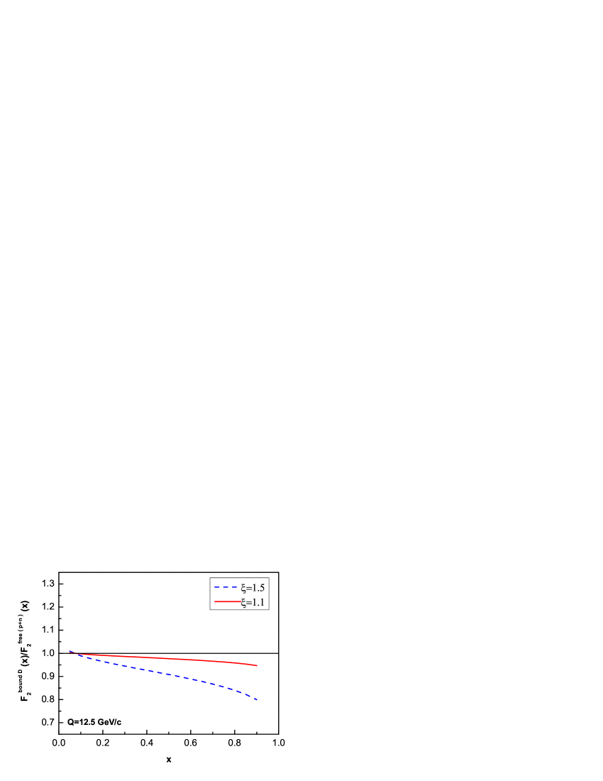
Figure 5: The ratio of bound deuterium $F_{2}^{\mathrm{D}}(x)$ compared to free $F_{2}^{\mathrm{p}+\mathrm{n}}(x)$. The solid (dashed) curve is the result with $\xi=1.1$ ($\xi=1.5$).

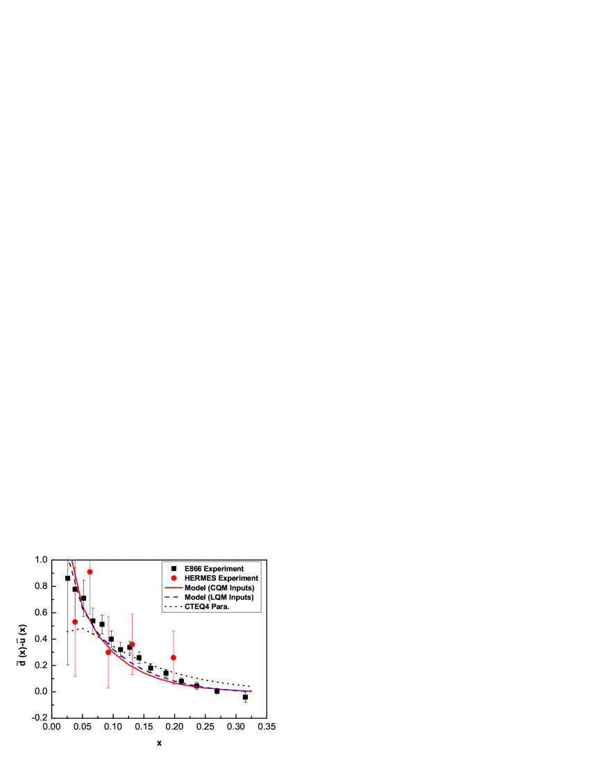
Figure 6: The distribution for $\bar{d}(x)-\bar{u}(x)$. The data are from HERMES HERMES and E866/NuSea E866 experiments. The solid and dashed curves are the model calculation results in the effective chiral quark model with the constituent quark model (CQM) and the light-cone quark-spectator-diquark model (LQM) as bare quark distribution inputs respectively. The dotted curve is the result from CTEQ4 parametrization. All the values are scaled to fixed $Q^{2}=54~{}\mathrm{GeV}^{2}/\mathrm{c}^{2}$.

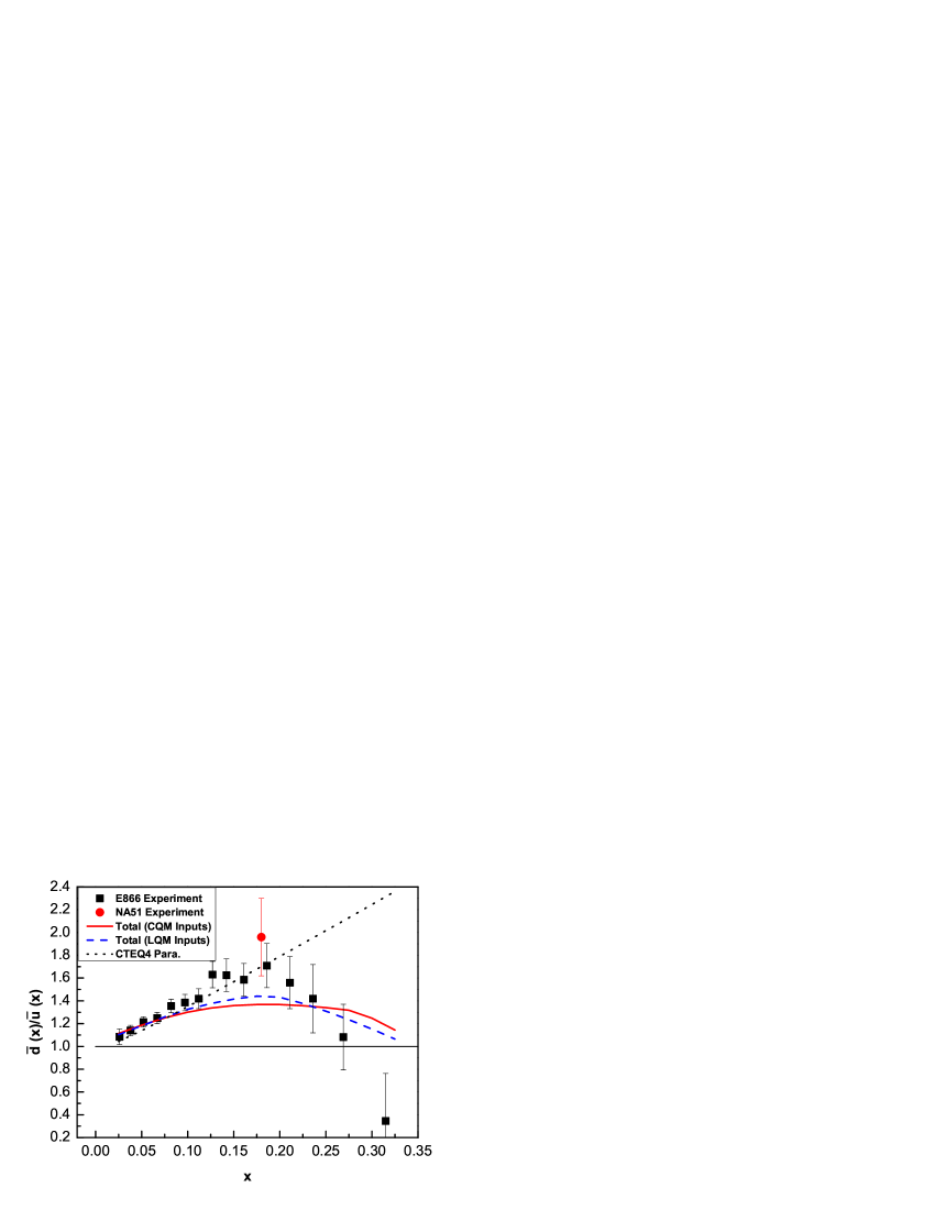
Figure 7: The distribution for $\bar{d}(x)/\bar{u}(x)$. The data are from NA51 NA51 and E866/NuSea E866 experiments. The solid and dashed curves are the model calculation results in the effective chiral quark model with the constituent quark model (CQM) and the light-cone quark-spectator-diquark model (LQM) as bare quark distribution inputs plus symmetric sea contributions. The dotted curve is the result from CTEQ4 parametrization. All the values are scaled to fixed $Q^{2}=54~{}\mathrm{GeV}^{2}/\mathrm{c}^{2}$.

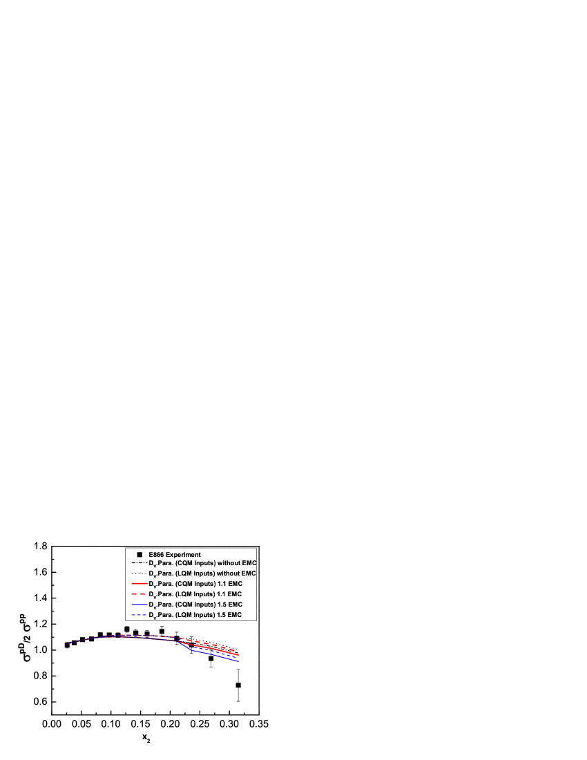
Figure 8: The Drell-Yan cross section ratio $\sigma^{\mathrm{pD}}/2\sigma^{\mathrm{pp}}$ versus $x_{2}$. The data are taken from E866/NuSea E866 experiment. $u(x)$, $\bar{u}(x)$, $d_{v}(x)$ are obtained by adding CTEQ4 parametrization and symmetric sea contributions. The thin dash-dotted and dotted curves are the results with $\bar{d}(x)$ derived from the chiral quark model with constituent quark model (CQM) and light-cone quark-spectator-diquark model (LQM) as bare quark distribution inputs without EMC effect. The thick solid and dashed curve are the corresponding results with EMC effect for the parameter $\xi=1.1$. The thin solid and dashed curves are the corresponding results with EMC effect for the parameter $\xi=1.5$.

5 RESULT AND CONCLUSION

In this work, we calculate the light flavor quark and antiquark distributions within the effective chiral quark model by using the constituent quark model and the light-cone quark-spectator-diquark model as inputs respectively, and revise the results by taking into consideration the symmetric nucleon sea contributions, the $Q^{2}$-evolution and the nuclear EMC effect. The distributions of $\sigma^{\mathrm{pD}}/2\sigma^{\mathrm{pp}}$ and $\bar{d}(x)-\bar{u}(x)$ match with the experimental data, and $\bar{d}(x)/\bar{u}(x)$ is compatible with the experiment at small $x$, while the behavior of $\bar{d}(x)/\bar{u}(x)$ in large $x$ region is different from the experimental result. However, the result directly measured in E866 experiment was only $\sigma^{\mathrm{pD}}/2\sigma^{\mathrm{pp}}$, whereas $\overline{d}(x)/\overline{u}(x)$ was derived indirectly from $\sigma^{\mathrm{pD}}/2\sigma^{\mathrm{pp}}$ with several assumptions. Although it is entirely possible that the analysis of E866/NuSea Collaboration was correct, it is also possible that the analysis of them was based on some excessive assumptions. For example, the assumption of $\bar{u}(x)+\bar{d}(x)$ fixed as parametrization may have a strong influence on the ratio $\bar{d}(x)/\bar{u}(x)$ derived from data of cross sections. In addition, it is worth noting that the nuclear EMC effect should be considered carefully when $x$ is large. Therefore, without ruling out these possibilities and considering all we discussed before carefully, the results of $\bar{d}(x)/\bar{u}(x)$ extracted from other quantities might be not so reliable as the results of $\sigma^{\mathrm{pD}}/2\sigma^{\mathrm{pp}}$. We also suggest an alternative procedure to derive $\bar{d}(x)/\bar{u}(x)$ and $\bar{d}(x)-\bar{u}(x)$ from the experimental data of $\sigma^{\mathrm{pD}}/2\sigma^{\mathrm{pp}}$. Thus it is important that more precision experiments should be carried out to enable more direct and accurate determination of sea quark and antiquark distributions.

References

• (1) K. Gottfried, Phys. Rev. Lett. 18, 1174 (1967).
• (2) New Muon Collaboration, P. Amaudruz et al., Phys. Rev. Lett. 66, 2712 (1991).
• (3) New Muon Collaboration, M. Arneodo et al., Phys. Rev. D 50, R1 (1994).
• (4) NA51 Collaboration, A. Baldit et al., Phys. Lett. B 332, 244 (1994).
• (5) Fermilab E866/NuSea Collaboration, E. A. Hawker et al., Phys. Rev. Lett. 80, 3715 (1998).
• (6) FNAL E866/NuSea Collaboration, J.-C. Peng et al., Phys. Rev. D 58, 092004 (1998).
• (7) FNAL E866/NuSea Collaboration, R. S. Towell et al., Phys. Rev. D 64, 052002 (2001).
• (8) HERMES Collaboration, K. Ackerstaff et al., Phys. Rev. Lett. 81, 5519 (1998).
• (9) For reviews, see, e.g., S. Kumano, Phys. Rept. 303, 183 (1998); G. T. Garvey and J. C. Peng, Prog. Part. Nucl. Phys. 47, 203 (2001).
• (10) B.-Q. Ma, Phys. Lett. B 274, 111 (1992); B.-Q. Ma, A. Schäfer, and W. Greiner, Phys. Rev. D 47, 51 (1993); H. Song, X. Zhang and B.-Q. Ma, Phys. Rev. D 82, 113011 (2010).
• (11) G. Preparata, P. G. Ratcliffe and J. Soffer, Phys. Rev. Lett. 66, 687 (1991).
• (12) S. D. Drell, T. M. Yan, Ann. Phys. 66, 578 (1971).
• (13) P. L. McGaughey et al., Phys. Rev. Lett. 69, 1726 (1992).
• (14) R. D. Field and R. P. Feynman, Phys. Rev. D 15, 2590 (1977).
• (15) D. A. Ross and C. T. Sachrajda, Nucl. Phys. B 149, 497 (1979).
• (16) F. M. Steffens and A. W. Thomas, Phys. Rev. C 55, 900 (1997).
• (17) J. D. Sullivan, Phys. Rev. D 5, 1732 (1972).
• (18) A. W. Thomas, Phys. Lett. B 126, 97 (1983).
• (19) S. Kumano, Phys. Rev. D 43, 59 (1991); D 43, 3067 (1991); S. Kumano and J. T. Londergan, Phys. Rev. D 44, 717 (1991).
• (20) E. M. Henley and G. A. Miller, Phys. Lett. B 251, 453 (1990).
• (21) A. Signal and A. W. Thomas, Mod. Phys. Lett. A 6, 271 (1991).
• (22) J. Stern and G. Cl$\acute{\mathrm{e}}$ment, Phys. Lett. B 264, 426 (1991).
• (23) W.-Y. P. Hwang, J. Speth, and G. E. Brown, Z. Phys. A 339, 383 (1991); W.-Y. P. Hwang and J. Speth, Phys. Rev. D 46, 1198 (1992).
• (24) S. J. Brodsky and B.-Q. Ma, Phys. Lett. B 381, 317 (1996).
• (25) S. Weinberg, Physica A 96, 327 (1979).
• (26) A. Manohar and H. Georgi, Nucl. Phys. B 234, 189 (1984).
• (27) E. J. Eichten, I. Hinchliffe, and C. Quigg, Phys. Rev. D 45, 2269 (1992).
• (28) M. Wakamatsu, Phys. Lett. B 269, 394 (1991).
• (29) P. V. Pobylitsa, M. V. Polyakov, K. Goeke, T. Watabe, and C. Weiss, Phys. Rev. D 59, 034024 (1999).
• (30) A. E. Dorokhov and N. I. Kochelev, Phys. Lett. B 259, 335 (1991); B 304, 167 (1993).
• (31) See, $e.g.$, Y.-H. Zhang, L. Shao, and B.-Q. Ma, Phys. Lett. B 671, 30 (2009); L. Shao, Y.-J. Zhang, and B.-Q. Ma, Phys. Lett. B 686, 136 (2010); and references therein. For a more realistic parametrization with a statistical model, please see, C. R. V. Bourrely, J. Soffer and F. Buccella, Eur. Phys. J.  C 41, 327 (2005).
• (32) R. C. Hwa and M. S. Zahir, Phys. Rev. D 23, 2539 (1981).
• (33) B.-Q. Ma, Phys. Lett. B 375, 320 (1996); B.-Q. Ma and A. Schafer, Phys. Lett. B 378, 307 (1996).
• (34) J. Ashman et al., Phys. Lett. B 206, 364 (1988); Nucl. Phys. B 328, 1 (1989).
• (35) T. P. Cheng and L.-F. Li, Phys. Rev. Lett. 74, 2872 (1995).
• (36) X. Song, J. S. McCarthy, and H. J. Weber, Phys. Rev. D 55, 2624 (1997).
• (37) Y. Ding, R.-G. Xu, and B.-Q. Ma, Phys. Lett. B 607, 101 (2005); Phys. Rev. D 71, 094014 (2005)
• (38) K. Suzuki and W. Weise, Nucl. Phys. A 634, 141 (1998).
• (39) S. Weinberg, Phys. Rev. Lett. 65, 1181 (1990).
• (40) See, e.g., A. Airapetian et al. [HERMES Collaboration], Phys. Rev. Lett. 92, 012005 (2004); A. Airapetian et al. [HERMES Collaboration], Phys. Rev. D 71, 012003 (2005).
• (41) A. Szczurek, A. J. Buchmann and A. Faessler, J. Phys. G 22, 1741 (1996).
• (42) M. Glück, E. Reya, and M. Stratmann, Eur. Phys. J. C 2, 159 (1998).
• (43) H. W. Kua, L. C. Kwek, and C. H. Oh, Phys. Rev. D 59, 074025 (1999).
• (44) R. C. Hwa and C. B. Yang, Phys. Rev. C 66, 025204 (2002); C 66, 025205 (2002).
• (45) S. J. Brodsky, T. Huang, and G. P. Lepage, in: Particles and Fields, eds. A. Z. Capri and A. N. Kamal (Plenum, New York, 1983), p. 143.
• (46) H. L. Lai et al., Phys. Rev. D 55, 1280 (1997).
• (47) J. J. Aubert et al., Phys. Lett. B 105, 322 (1981).
• (48) CERN NA2/EMC, J. J. Aubert et al., Phys. Lett. B 123, 275 (1983).
• (49) E139, R. G. Arnold et al., Phys. Rev. Lett 52, 727 (1984).
• (50) C. H. Llewellyn Smith, Phys. Lett. B 128, 107 (1983).
• (51) M. Ericson and A. W. Thomas, Phys. Lett. B 128, 112 (1983).
• (52) R. L. Jaffe, Phys. Rev. Lett. 50, 228 (1983).
• (53) C. E. Carlson, T. J. Havens, Phys. Rev. Lett. 51, 261 (1983).
• (54) H. J. Pirner and J. P. Vary, Phys. Rev. Lett. 46, 1376(1981)
• (55) F. E. Close, R. G. Roberts, and G. G. Ross, Phys. Lett. B 129, 346 (1983).
• (56) R. L. Jaffe, F. E. Close, R. G. Roberts, and G. G. Ross, Phys. Lett. B 134, 449 (1984).
• (57) F. E. Close, R. L. Jaffe, R. G. Roberts, and G. G. Ross, Phys. Rev. D 31, 1004 (1985).
• (58) O. Nachtmann and H. J. Pirner, Z. Phys. C 21, 277 (1984).
• (59) B. Lu and B.-Q. Ma, Phys. Rev. C 74, 055202 (2006); Y. Zhang, L. Shao and B.-Q. Ma, Nucl. Phys. A 828, 390 (2009); and references therein.