The Infrared Properties of Embedded Super Star Clusters: Predictions from Three-Dimensional Radiative Transfer Models

Abstract

With high-resolution infrared data becoming available that can probe the formation of high-mass stellar clusters for the first time, appropriate models that make testable predictions of these objects are necessary. We utilize a three-dimensional radiative transfer code, including a hierarchically clumped dusty envelope, to study the earliest stages of super star cluster evolution. We explore a range of parameter space in geometric sequences that mimic the hypothesized evolution of an embedded super star cluster. The inclusion of a hierarchically clumped medium can make the envelope porous, in accordance with previous models and supporting observational evidence. The infrared luminosity inferred from observations can differ by a factor of two from the true value in the clumpiest envelopes depending on the viewing angle. The infrared spectral energy distribution (SED) also varies with viewing angle for clumpy envelopes, creating a range in possible observable infrared colors and magnitudes, silicate feature depths and dust continua. General observable features of cluster evolution differ between envelopes that are relatively opaque or transparent to mid-infrared photons. For optically thick envelopes, evolution is marked by a gradual decline of the $9.8$µm  silicate absorption feature depth and a corresponding increase in the visual/ultraviolet flux. For the optically thin envelopes, clusters typically begin with a strong hot dust component and silicates in emission, and these features gradually fade until the mid-infrared PAH features are predominant. For the models with a smooth dust distribution, the Spitzer MIPS or Herschel PACS [$70$]-[$160$] color is a good probe of the stellar mass relative to the total mass, or star formation efficiency. Likewise, the IRAC/MIPS [$3.6$]-[$24$] color can be used to constrain the R_in and R_out values of the envelope. However, clumpiness confuses the general trends seen in the smooth dust distribution models, making it harder to determine a unique set of envelope properties. Nevertheless, good diagnostic colors were found for each of the input parameters: again, the [$70$]-[$160$] color can be used to separate models with different star formation efficiencies; the Spitzer IRAC/MIPS [$8.0$]-[$24$] color is able to constrain R_in and R_out values; and the IRAC [$3.6$]-[$5.8$] color is sensitive to the fraction of the dust distributed in clumps. Finally, in a comparison of this model set to IRAS data of ultracompact Hii regions, we find good agreement, suggesting that these models are physically relevant, and will provide useful diagnostic ability for datasets of resolved, embedded SSCs with the advent of high-resolution infrared telescopes like James Webb Space Telescope.

1 INTRODUCTION

Super star clusters (SSCs) are massive young star clusters with high stellar densities ($\gtrsim 10^{3}$ stars pc^-3) that form under extreme pressures, often found in merging galaxy systems, galactic nuclei, and blue compact dwarf galaxies (Whitmore, 2002, and references therein). With masses typically in excess of $10^{5}M_{\sun}$, they are the most massive type of stellar cluster known. Studies of the most nearby analogues Westerlund $1$ (Clark et al., 2005) and R$136$ (Bosch et al., 2009) show that these objects are consistent with expectations that they are globular cluster progenitors; this expectation is strengthened by numerous studies of SSC populations outside the Local Group (e.g. Schweizer et al., 1996; Holtzman et al., 1992; O’Connell et al., 1994; Conti & Vacca, 1994; Johnson et al., 1999). Because of their high density of massive stars, models show that SSCs have the ability to disperse metals from supernovae ejecta to large distances, trigger further star formation episodes, and act as a launching mechanism for super-galactic winds (Wünsch et al., 2008; Murray et al., 2010). Therefore SSCs can have a major impact on their host galaxies.

Tracking the early evolution of SSCs requires long wavelength observations due to the dust-enshrouding birth envelopes that surround them at young ages. Embedded SSCs were first detected in the radio (e.g. Kobulnicky & Johnson, 1999; Turner et al., 2000) in low-metallicity blue compact dwarf galaxies (BCDs) as compact sources with high ionizing fluxes. Numerous other examples have also been found in the infrared, in starbursts such as Arp $220$ (Shioya et al., 2001) and again in BCDs (Sauvage & Plante, 2003).

Radio observations have confirmed the masses of embedded SSCs to be in the range found for their optical counterparts. Furthermore, the calculated high ionizing fluxes are equivalent to hundreds or thousands of O-stars and electron densities are $\sim 10^{3-4}$cm^-3 (Beck et al., 2002; Johnson et al., 2003; Johnson & Kobulnicky, 2003). These densities are similar to those found in Galactic HII regions, but are significantly lower than typical densities associated with Active Galactic Nucleus Broad Line Regions ($>10^{8}$cm^-3) suggesting that SSCs are also heated by young stars in a starburst environment, and not AGN.

Despite advances made this last decade in understanding embedded SSCs as starburst events, their early evolution is still poorly understood. Properties such as the mass and physical size of the clouds from which they are formed and the amount of gas that is turned into stars (i.e. the star formation efficiency; Ashman & Zepf, 2001) are not well-constrained. In addition, the most recent radio, near-infrared, and ultraviolet data on these objects suggest that the thick envelopes are porous, allowing a significant fraction of UV light to leak from the system (Reines et al., 2008; Johnson et al., 2009; Thuan et al., 2005). This project is a first attempt at modeling the infrared spectral energy distributions of embedded super star clusters. By investigating a large variation in the values of the input parameters in a hierarchically clumpy and porous envelope, these models can be used to constrain the dusty envelope geometry and star formation efficiency of embedded super star clusters.

The decision to model embedded SSCs in the infrared is based on the fact that they are most visible in the infrared and radio; at these young ages, hot stars heat the dust in the circum-cluster envelope and excite free-free radio emission inside the Hii region. Therefore these wavelengths are essential for studying the dust properties during the embedded phase, the dust mass, and the envelope geometry. The radiative transfer models presented in this work offer predictions about what we expect embedded SSCs to look like in the infrared and what wavelength observations offer the best diagnostic capability. With telescopes like JWST on the horizon, its high spatial resolution and mid-infrared sensitivity making it far better than existing infrared space facilities (Sonneborn, 2008), we may finally be entering a period when questions about initial dust mass and geometry of a SSC’s embedded phase can be answered on a global scale. In the near term, observations using Herschel and Spitzer may be used to probe unresolved embedded SSCs, and these models can be used to estimate their physical size and geometry.

In this paper we present simulated infrared images, SEDs, and colors of embedded SSCs along a geometric sequence that mimics the evolution of a young embedded super star cluster. We discuss the models in detail in §2, then present model images, SEDs and colors in §3. We compare unresolved populations to the models in §4, discuss the limitations of these models when comparing to resolved populations in §5, and conclude in §6.

2 MODELS

2.1 The Radiative Transfer Method

The models presented in this paper calculate radiative transfer from thermal dust grains and stochastic small grains, and scattering from the dust. The code simulates a three-dimensional geometry, and is based on previous work on thermal dust grains in two dimensions (see Whitney et al., 2003; Chakrabarti & Whitney, 2009), updated to include three dimensions and clumpy dust distributions (Indebetouw et al., 2006), and stochastic emission from polycyclic aromatic hydrocarbons and very small grains (PAHs/VSGs; Wood et al., 2008).

The code uses a Monte-Carlo technique that issues ‘photon packets’ into a dusty envelope from a central source. Packets that encounter large grains either change the temperature in the grid space in which the encounter occurs, according to the prescription of Lucy (1999), or are scattered according to a modified Henyey-Greenstein function (Cornette & Shanks, 1992). A small number of packets encounter PAHs/VSGs, and are re-emitted according to emissivity templates from Draine & Li (2007); see Wood et al. (2008) for details about emission from PAHs/VSGs in our models.

Embedded SSCs are believed to have porous envelopes that allow a significant portion of the ultraviolet (UV) light to escape from the system (supporting observational evidence is provided in §2.5 from Thuan et al., 2005; Reines et al., 2008; Johnson et al., 2009). To account for this fact, we have included a hierarchically clumped density structure for the dusty envelope, using the prescription of Elmegreen (1997).

In order to confine the parameter space investigated in this model set, we have varied only four input parameters that most influence the output spectral energy distribution: the inner and outer dust radii in a spherical geometry; the mass in stars divided by the total cluster mass (i.e. the ‘star formation efficiency’ or SFE; Ashman & Zepf, 2001); and the fraction of dust that is smoothly, as opposed to fractally, distributed. The many other parameters that remain fixed, such as the central star cluster mass, the IMF, the central source luminosity and age, the dust species used, the volume fractal dimension adopted, and the radial dust distribution exponent, are all described in §2.2 to §2.4.

2.2 The Dust Composition

We use the standard dust model size distribution derived in Kim et al. (1994) that fits an extinction curve with R${}_{V}=4$ using the prescription of Cardelli et al. (1989). The size distribution is not a simple power law, but is derived from a Maximum Entropy Method solution, which gives the best solution compatible with the extinction data. The chosen R_V value has been found to be appropriate for the more dense regions of molecular clouds (Whittet et al., 2001) and therefore we make the assumption that it will also fit embedded SSCs.

We adopt the dielectric functions of astronomical silicate and graphite grains from Laor & Draine (1993). Our grain model includes a layer of water ice on the grains, covering the outer $5$% in radius. The ice mantle increases the opacity of the grains at all wavelengths, but the change is most pronounced longward of 35µm. The slope of the opacity with wavelength is the same in the infrared for grains with and without the ice mantle, so any error introduced by the inclusion of an ice mantle is a scalar factor at the wavelengths of concern in this paper. The ice dielectric function is from Warren (1984).

The PAHs/VSGs are templates from Draine & Li (2007). The energy density of the radiation field relative to the interstellar radiation field (ISRF) can vary between $0.5\leq U\leq 10^{7}$ and the ionization fraction is that used in Draine & Li (2007) to constrain the models to reproduce the observed Milky Way spectrum. Only grains that are $\leq 200$Å  in size are considered small grains. Grains larger than this are assumed to thermalize after photon interactions, and are therefore considered large grains. The PAH/VSG mass fraction in dust used in this paper is $3.55$%, which is the average value found for $65$ galaxies in the SINGS survey (Draine et al., 2007). This is therefore an acceptable value to expect for extragalactic embedded SSCs.

2.3 The Central Source

In these models, the central cluster is treated as a point source with the spectrum of a $10^{6}$ M_☉ star cluster, produced by the Starburst99 spectral synthesis models (Leitherer et al., 1999). The input metallicity is solar and the initial mass function is a Salpeter IMF (Salpeter, 1955); changing these parameters was found to have little effect on the overall shape of the resulting infrared SED, validating the decision to hold them constant. The age is set to $1$ Myr throughout the geometric sequence to ensure that the UV luminosity remains constant. Since evolution is expected to take place in less than three or four million years, prescribing a fixed age is warranted - see §2.5 for a discussion about the evolutionary pace for embedded super star clusters. The instantaneous starburst mode was chosen, without continuum emission. The luminosity of the source is $1.6\times 10^{9}$L_☉.

2.4 The Envelope Properties

The dust and gas around the central source is distributed spherically with variable inner and outer radii and envelope mass. The initial envelope mass is set for star formation efficiencies (SFEs) of $5$%, $10$%, $15$%, $25$%, and $50$%, which is a large range of possible values based on observations of star-forming regions (Bonnell et al., 2010; Murray et al., 2010). The dust can be distributed fractally and smoothly, and the percentage of dust that is smoothly distributed is varied from between $100$% smooth to $1$% smooth (i.e. $0$% to $99$% clumpy).

The models mimic a cluster’s evolution by moving the inner radius out towards the outer radius in a geometric sequence; Table 1 lists the sequence for the three possible outer radii we have chosen, and Figure 1 shows how the geometric progression roughly follows what is expected for a real SSC. At very young ages, each star will realistically inhabit its own compact Hii region, but as the cluster evolves, these compact regions will grow and merge into a single, large cavity. Assuming a stationary stellar wind as in the semi-analytical and numerical models presented by Tenorio-Tagle et al. (2007), this cavity will grow and disperse, eventually leaving the central SSC exposed. The initial inner radius of the models, correlated to intra-cluster dust, is $0.1$pc, and moves out to the outer radius, which remains fixed.

The SFE values from $5$% to $50$% presume initial cocoon masses in the range $1.9\times 10^{7}$M_☉ down to $1\times 10^{6}$M_☉. For a given SFE value and outer radius, the average mass density is constant with radius, so that the mass of the shell in a geometric sequence scales with the inner and outer radii as: $M\propto R_{out}^{3}-R_{in}^{3}$. The average mass densities range from $10^{5}$ cm^-3 at the densest to $10$ cm^-3 at the least dense, where the densest models are for a SFE of $5$% and an outer radius of $25$pc while the least dense models are for a SFE of $50$% and an outer radius of $100$pc.

The envelope is assumed to have a standard dust-to-gas ratio of $0.01$. It is furthermore seeded with PAHs/VSGs to a depth equal to $A_{V}=1.5$ from the ionizing source. This is because the UV flux is sufficiently attenuated after this depth that we expect very little UV heating of small grains in the rest of the envelope. Comparisons between models run with PAHs/VSGs throughout the dusty envelopes and models PAHs/VSGs in to a depth of $A_{V}=1.5$ show that PAH/VSG emission changes only slightly for models where $A_{V}\lesssim 250$.

There are five clumpy dust fractions presented: $0$, $0.1$, $0.5$, $0.9$, & $0.99$ clumpy. The spread in clumpy fraction is the complete range of conceivable clumpy values that could be found. The volume fractal dimension was chosen as the best value from Elmegreen (1997) which matched the turbulent intercloud medium, D=2.3. The fractal length L is taken to be 3.792 so that the maximum density of the clumps can be computed per hierarchic level, $\rho(h)=L^{(3-D)h+HD}$ where $h$ is the hierarchical level in question and $H$ is the maximum hierarchical level, which we have set equal to five; higher $H$ values create fractal sizes smaller than the resolution elements in our three-dimensional grid.

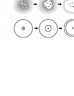
Figure 1: A cartoon illustrating the early stages of a super star cluster’s evolution and our corresponding model estimates. The smallest inner radius presented in this paper, $R_{\rm in}=0.1$ pc, is likely to correspond to intra-cluster dust in a real cluster (left-most figure), which will only exist while the constituent stars still have individual cocoons.

2.5 Supporting Observational Evidence for the Model Parameter Choices

The model parameters were chosen to be consistent with observations of embedded SSCs, and the parameter space is corroborated with observational evidence from the literature in this section.

With regard to dust grains types, the PAH models from Draine & Li (2007) are the most suitable available to date. Ongoing research (Draine & Li, 2007; Galliano et al., 2008) that accounts for different PAH ionization fractions and redder exciting sources than those used here would likely change individual PAH band fluxes. However, since we are not interested in PAH ratios in this work, the inclusion of these processes does not impact the results of this study.

The ice mantle on the dust grains is suitable for dense, cold regions, such as young star formation regions, where a large part of the dust is not being heated by the embedded stars and the water-ice cannot be sublimated from the grains. At any optical depth it has been shown that the water-ice features will be masked and therefore hard to detect (Robinson & Maldoni, 2010). Since there is observational evidence for water associated with compact, young star clusters (Brogan et al., 2010) and the slope of the opacity functions with and without water ice are the same, we have left the dust with ice mantles throughout the entire geometric sequence.

Fixing the cluster age is based on upper limits of the time it takes for a cluster to emerge from its envelope. Observations with HST show optically visible clusters with ages of just a few Myr (e.g. Johnson et al., 2000). Radio observations have also suggested the same approximate age, so we can assume a fiducial emergence timescale of about three Myr for a super star cluster (Whitmore, 2002; Kobulnicky & Johnson, 1999). Since the UV continuum, which most affects the resulting infrared SED, does not significantly change between ages of $0$ and $~{}3$-$4$ Myr, setting the cluster age to $1$ Myr throughout the sequence is warranted in order to limit the number of free parameters.

The models are run under the assumption that the central star cluster is a point source and the envelope is perfectly spherical; this is a necessary simplification to confine the parameter space in this study. However, the high stellar densities and small half-light radii discovered for optically-visible SSCs (Tacconi-Garman et al., 1996; de Marchi et al., 1997) suggest that the central source is fairly localized in its formation envelope. Furthermore, placing dust to within $0.1$pc of the central point source will produce the high dust temperatures expected from intracluster dust in a real embedded SSC. Dust sublimation is not a concern even for these most embedded model phases: the dust sublimation radius, assuming a sublimation temperature of $1600$K, is $0.03$pc, well within the smallest inner radius value adopted.

The outer radii of $25$, $50$, and $100$pc were chosen based on estimates from observational results. Vacca, Johnson, & Conti (2002) model infrared and radio observations of ‘ultra-dense’ Hii regions in Henize 2-10 as scaled-up versions of Galactic ultra-compact Hii regions to derive their radial size. Hunt et al. (2005) based their estimates on models of global dwarf galaxy SEDs for which the radii of the actively star-forming regions are derived based on infrared luminosities and temperatures.

Lastly, in order to be consistent with the growing body of evidence that suggests that the ISM is clumpy in a large variety of environments, a clumpy envelope was included around the central star cluster. That the ISM is not uniform is well established (e.g. Verschuur, 1995; Elmegreen & Efremov, 1997; Kim et al., 2008). In star formation environments, recent work has begun to show that the same is true. Thuan et al. (2005) shows that the molecular hydrogen in a BCD galaxy is clumpy because emission is visible in the near-IR, which is sensitive to dense H₂, but not in the UV, which is sensitive to diffuse H₂. Reines et al. (2008) and Johnson et al. (2009) show that for different clusters, more than $40$% and $50$% of the UV flux is detected outside the embedded sources. This could either be because the ISRF is very strong around the clusters or because there is light leaking from the clusters. Most recently, model-dependent results by Eldridge & Relaño (2010) shows that about $50$% of the ionizing flux is leaving the giant Hii region NGC$604$, though this latter result is highly dependent on ages derived from observations of Wolf-Rayet stars.

3 RESULTS

3.1 Simulated Images

Images of the clusters at several stages along the geometric sequence are shown in Figure 2 in near-IR (J, H, and K bands), mid-IR (Spitzer IRAC 3.6µm, 4.5µm, and 8.0µm  bands; Fazio et el., 2004), and far-IR (Spitzer MIPS 24µm, 70µm, and 160µm bands; Rieke et al., 2004) light from left to right. They were created from the SFE $=10$% models with an outer radius of $50$pc, clumpy dust fraction of $0.9$ and inner radii of $1$, $5$, $20$, and $45$pc from top to bottom.

One of the striking features of these simulations is that a significant amount of the near-IR light can escape the clumpy envelope, as seen by the scattered light on the inside of the cloud surfaces. Due to the scattered light, the near-IR images appear blue in color, because scattering favors bluer photons (in this case, J-band photons are scattered more regularly than K-band photons). The mid-IR band images, sensitive to warm dust and PAH/VSG emission, appear red because of the dominant PAH feature and high dust continuum in the 8µm band. As the inner radius moves outward, the MIR colors become more red because the inner dust temperature becomes lower, removing what little hot dust radiation in the small-wavelength bands there was. Additionally the hole appears to be the brightest feature in the mid-IR because the shell is being lit up by the central source. The far-IR bands probe both sides of the infrared dust peak, with the 24µm  emission showing hotter dust and 70 and 160µm  bands showing cold dust emission. Since the dust peak is typically near 70µm, these images therefore appear green.

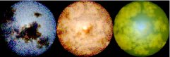
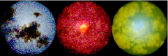
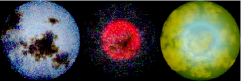
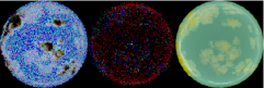
Figure 2: Simulated color images for a geometric (pseudo-evolutionary) sequence of a natal SSC for a SFE of $10$%, outer radius $=50$ pc, and clumpy fraction $=90$%. Images are shown for an inner radius of the cocoon of $1$ pc, $5$ pc, $20$ pc, and $45$ pc, from top to bottom respectively. The colors shown are for combinations of J, H,and K (left), IRAC $3.6$µm, $4.5$µm, and $8$µm (middle), and MIPS $24$µm, $70$µm, and $160$µm (right).

3.2 The Change in Ultraviolet Flux with Clumpy Dust Fraction

Motivated by observations suggesting that roughly $50$% of the UV flux leaks from embedded star clusters (see Reines et al., 2008; Johnson et al., 2009, for details on the observations), we plot the fraction of UV light lost as a function of the R_in/R_out ratio for the $99$% clumpy models in Figure 3.

Figure 3 shows that R_in/R_out ratios $\gtrsim 0.5$ generally reproduce the results, depending on the SFE and R_out values adopted. The very high SFE values, such as $50$%, always allows a large fraction of the ultraviolet photons out of the envelope because of its low optical depth. The clumpiness will also have an effect on the fraction of UV light leakage, and generally less light will leak from envelopes with smaller clumpy fractions.

Since the radio sources studied in Reines et al. (2008) and Johnson et al. (2009) are obscure, however, their findings are probably for low-SFE, moderately evolved regions where the optical extinction for a corresponding model is about A${}_{V}\thicksim 30-50$ on average. The UV light leakage would therefore take place along those sightlines exhibiting minimal extinction, A${}_{V}\lesssim 1$.

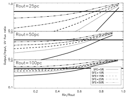
Figure 3: The fraction of UV light that escapes from the $99$% clumpy embedding envelope as a function of R_in/R_out. The horizontal line is at a value of $0.5$, signifying $50$% of the UV flux is not being reprocessed by the dust, and is only meant to help guide the eye. The solid line is for a SFE of $5$%, dotted line for $10$%, dashed line for $15$%, dash-dot line for $25$%, and dash-dot-dot for $50$%.

3.3 Infrared Variation with Viewing Angle

The clumpy dust distribution creates variations in infrared luminosity and certain spectral features depending on the viewing angle. In a general sense, clumpier media show the most variation in spectral features and luminosity compared to smoother media.

Figure 4 demonstrates how the infrared luminosity derived from a random sightline will be incorrect due to a clumpy envelope. The infrared luminosity inferred from a single sightline observation, plotted as stars in the figure and defined as the $3$-$1000$µm  integrated luminosity, can vary from roughly half to nearly twice the true infrared luminosity for a clumpy dust distribution. The true infrared luminosities are plotted as diamonds and are the infrared luminosities summed over all viewing angles for a model. For smooth dust distributions with thick envelopes, the input central source luminosity is equal to the true infrared luminosity. The infrared luminosities are compared to the stellar cluster’s input luminosity of $1.604\times 10^{9}$L_☉, plotted as the solid horizontal line.

If a clump is along the line of sight in front of the central source, the optical depth will appear to be high and the $9.8$ and $17$µm  silicate absorption features will be deeper in the infrared spectrum. However, clumps that are behind the central source will reflect light, and silicate emission features will therefore be evident. This is illustrated in Figure 5, which shows that the features of the infrared spectrum of a source inside a clumpy envelope are highly sightline-dependent. The average spectrum is also shown for comparison.

Figure 4: The computed infrared luminosity (3-1000µm) plotted versus the fraction of dust that is in clumps for an optically thick (top) and an optically thin (bottom) model. R_out is $25$pc for both panels. The horizontal line is the input stellar cluster luminosity, which matches the $L_{IR}$ for optically thick models. The $L_{IR}$ computed along each sightline, assuming a spherical, smooth distribution, is plotted with stars, while the $L_{IR}$ values determined by adding up all sightlines for a model are shown as diamonds (this is the correct infrared luminosity). The clumpier models, as well as showing a larger dispersion in computed infrared luminosity values, also exhibit lower infrared luminosities in general, because the clumpy envelope allows ultraviolet photons to exit the envelope (see Figure 3).

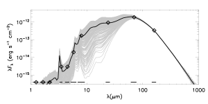
Figure 5: The variation of the SED for a given model due to the viewing angle of the observer. For this example, the model shown has R${}_{\rm out}=25$ pc, R${}_{\rm in}=3$ pc, a clumpy fraction of 0.90, and a 10% SFE. The mean SED is shown with a black line, and the near-IR and Spitzer observing bands are indicated with diamonds, with $\Delta\lambda$ for each band given at the bottom.

3.4 Spectral Energy Distribution Properties

The output spectral energy distributions all generally have four components: ($1$) an extincted stellar spectrum from the central source; ($2$) thermal dust emission that peaks between $40$ and $70$µm; ($3$) silicate emission or absorption features; and ($4$) the PAH features visible in the mid-IR. Figure 6 shows the smooth dust SEDs for a geometric sequence as an example of how these four main components are expected to change as the cluster evolves. The geometric sequences for all SFE and R_out values are given in Figures 7 and 8 for the smooth and $99$% clumpy dust distributions. In Figure 8, the gray spectra are individual sightline SEDs for each R_in value, while the colors are the sightline-averaged values.

For the most dense models, including low SFE values and small R_in values, the starlight is largely absorbed by the envelope. For clumpy envelopes, many sightlines allow optical and UV photons to pass through so that a stellar continuum is visible, while the clumps have very high extinction values. For smooth dust distributions the starlight is largely absorbed along all sightlines. The A_V values for smooth distributions compared to the average values and ranges found in clumpy solutions, are listed in Table 2 for the R${}_{in}=0.1$pc models. The average A_V values for evolved stages in the geometric sequence are relatively small for all models (roughly less than $2$), hence the spectra of clumpy and smooth models at high SFE value and large inner radii are similar.

The wavelength of the far-IR peak of the thermal grain emission depends on the predominant temperature of the dust in a model envelope. For the high column density envelopes, which have low SFE values and small R_in values, the UV light is absorbed in the inner portions of the envelope so that much of the envelope remains quite cold. Therefore, low SFE values and small R_in values tend to produce infrared peaks at about $60$µm. For the optically thin models with high SFE values and large inner radii, a large proportion of the dust is being heated by the cluster, so the far-IR peak moves to shorter wavelengths.

Silicate absorption is directly proportional to the optical depth, so that the deepest silicate features appear in the largest column-depth models. Silicates in emission, as was described in § 3.3, appear in clumpy models where sightlines include dust clumps illuminated behind the central source, which re-emit absorbed starlight as $10$µm  light that is unblocked by any intervening clouds.

The PAH features are almost ubiquitous in the model SEDs. The early stages in the geometric sequence appear to have reduced emission from the PAHs for two reasons. The first reason is that for the high density models, there is very little volume from which the PAHs can be excited; PAHs are only excited by UV photons to a depth of A${}_{V}=1.5$. The second reason is because the thermal hot dust component dominates the mid-IR flux for the early stage models, which lowers the measured equivalent widths of these features. For later stages on the geometric sequence, the PAH emission is relatively constant along the sequence because as the ultraviolet flux on the inner surface of the envelope decreases as r^-2, the surface area available to excite PAH molecules increases as r².

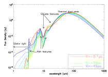
Figure 6: The spectra shown are along the geometric sequence in Table 1 for R${}_{out}=50$pc and a smooth dust distribution. As R_in increases towards R_out, the silicate features, most noticeably the one at $\sim 9.8$µm, become shallower. The PAH features are about the same throughout the sequence. The envelopes with small inner radii are more opaque to short-wave radiation and reprocess it to longer wavelengths. Therefore less flux between $1$-$5$ µm  is measured and more flux at $100$ µm, shifting the peak of the SED to the red. The stellar light is less extincted at larger R_in values.

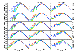
Figure 7: The infrared SEDs of all of the geometric sequences using a smooth dust distribution are shown; the range in R_in values from small to large are as in Figure 6.

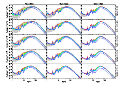
Figure 8: The infrared SEDs of all the geometric sequences using a $99$% clumpy dust distribution, with the sightline-average data shown in colors as in Figures 6 and 7 and the individual sightline data shown in gray scale.

3.5 Infrared Colors as Tracers of the Input Parameters

The model SEDs have been convolved with numerous filter sets for comparison to photometric observations. These include the four IRAS bands ($12$, $25$, $60$ and $100$µm), three standard near-IR bands (J, H, and K), Spitzer IRAC bands ($3.6$, $4.5$, $5.8$, and $8.0$µm), Spitzer MIPS bands ($24$, $70$, and $160$µm), Herschel PACS bands($70$, $100$, and $160$µm) and Herschel SPIRE bands ($250$, $350$, and $500$µm).

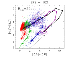
Figure 9: Using the mid-IR Spitzer/IRAC colors, the geometric sequence for R${}_{out}=25$pc and SFE$=10$% is shown for smooth models (black line), $10$% clumpy models (purple), $50$% clumpy models (blue), $90$% clumpy models (green), and $99$% clumpy models (red). The geometric sequences begin towards the bottom with R${}_{in}=0.1$pc and follow the arrows around the turn-around to their termination at R${}_{in}=24$pc. The solid lines and diamonds trace out the sightline-averaged colors, and the dots represent individual sightlines. While even the individual average tracks often overlap, the different sightlines add a significant uncertainty to any interpretation of these data.

As an example of how colors can be used to plot the data, we show the IRAC colors for the R${}_{out}=25$pc and SFE$=10$% models for all clumpiness values and all R_in values in Figure 9. There are degeneracies in the model average values at late evolutionary stages, and the individual sightlines make the interpretation of data extremely difficult.

Because the clumpy dust distributions create degeneracies in the SEDs, diagnostics to recover the input parameters were developed using the smooth dust distribution models first. In Figure 10 the [$3.6$]-[$24$] color is plotted against the R_in/R_out. Red, green, and blue are used to designate models with different R_out values (red, green, and blue for $100$, $50$, and $25$pc, respectively), and the plotting symbols are for the five different SFE values considered. Although there is significant overlap between the colors, the tracks are separate over most of the R_in/R_out values for each individual SFE value. The [$70$]-[$160$] color can be used to roughly determine the SFE value as shown in Figure 11; the bars represent the model dispersions. There is significant overlap between dispersion in SFE values of $10$% to $25$%, but [$70$]-[$160$] values of $>0.9$ represent very low SFE values ($<10$%), values between $\sim-1.0$ and $-1.5$ represent SFE values between $10$% and $25$%, and values $>-1.6$ will be for SFE of $50$% or greater.

Colors that can best be used to recover the input parameters for the entire, clumpy suite of models were also investigated. Given that the value of the input parameters and the viewing angle can both significantly change an embedded source’s SED and colors, there is a need to determine which, if any, photometric measurements can be used to reliably constrain the physical geometry. For a given input parameter (SFE, clumpiness, R_in, or R_out), the following calculation was made: for each color, the mean color and standard deviation was measured with the input parameter fixed and everything else (i.e. the other input parameters and all viewing angles) variable. This was done at each fixed input parameter value (e.g. for each of the five different SFE values). Finally the difference in the means is divided by the greatest of the standard deviations - this is a measure of how much the input parameter affects the color, compared to the other input parameters and the viewing angle ambiguities.

This analysis is related to a Principal Component Analysis, but adjusted to our goal of finding the minimal set of colors with maximal physical diagnostic power. Rather than solving freely for eigenvectors of the model set in color space, which may not directly correspond to the physical variables, we hypothesize that a principal component exists for which the eigenvalue would directly correspond to a physical parameter, and then measure the projection of that hypothetical component onto each of our color axes. This process allows of course that there is no such ‘physically diagnostic principal component,’ in which case the variation of all colors with the physical parameter would be small compared to the standard deviation in the color due to other causes.

Figures 12 to 14 are plots of infrared color versus infrared color where the grayscale shows the value of the quotient for determining the best diagnostic color described above. Values in the figures near zero indicate little spread in the average color for each input parameter value, while values at the maximum have relatively large spreads in average color values across the input parameter values, as well as small standard deviations from the mean. These are therefore the best colors for separating input parameter values: ($1$) [$70$]-[$160$] for SFE (Figure 12); ($2$) [$3.6$]-[$5.8$] for fraction of dust in a clumpy distribution (Figure 13); and ($3$) [$8.0$]-[$24$] for both R_out and the R_in/R_out ratio (Figure 14).

Figures 15, 16, and 17 plot these most useful colors’ average values and standard deviations for the whole suite of models versus the input parameters. For SFE (Figure 15), as with the smooth dust distribution models, there is overlap in the [$70$]-[$160$] color between the various SFE values. The overlap is still most significant between $10$ and $25$%, for which color values between $-1.5$ and $-0.9$ would all be valid. Color values above $-0.9$ match the $5$% SFE, and color values below $-1.5$ match the $50$% SFE. For the smooth dust fraction, within the error bars in the [$3.6$]-[$5.8$] versus smooth dust fraction plot (Figure 16) the color values are still degenerate, and using thermal radio data (such as was presented in Reines et al., 2008) is a more reliable metric for determining the fraction of ultraviolet light lost from an embedded star cluster. However, because the standard deviations in color of the clumpiest fractions are small compared to the smooth models (due to the large differences in the input parameter values being explored), a large, statistical study of embedded star clusters, for which average color values and standard deviations could be computed, could potentially be used to discern between the different smooth dust fraction values. For R_in/R_out (Figure 17), colors are still intractable for small R_in/R_out values. For R_in/R${}_{out}>0.4$, the [$8.0$]-[$24$] can be used both to distinguish between different R_in/R_out values and to distinguish between the different R_out values.

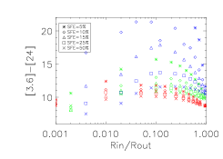
Figure 10: The [$3.6$]-[$24$] color is plotted versus the ratio of the inner and outer envelope radii for the three different outer radius values considered, $25$, $50$, and $100$pc (shown in blue, green, and red, respectively) using the smooth dust distribution models only. If the star formation efficiency (SFE) can be determined using the [$70$]-[$160$] color as shown in Figure 11, then the R_in/R_out value can be estimated using this plot.

Figure 11: The [$70$]-[$160$] color is used to separate different SFE values for the models with a smooth dust distribution. The bars shown are the dispersion and there is a fair bit of overlap between the models. One can only expect, therefore, to be able to roughly determine the SFE for the smooth models.

Figure 12: Determining the best color (y-axis magnitude minus x-axis magnitude) for recovering the star formation efficiency (SFE). In order to determine the best color for discriminating between different SFE values, this calculation was made: the spread in the mean color values between the different SFE values was divided by the greatest standard deviation of each SFE value was computed. The maximum resulting value is the most discriminating color (see §3.5). Each color is the y-axis magnitude minus x-axis magnitude, and the best color was found to be [$70$]-[$160$]. How well this ‘best’ color helps to determine the SFE is shown in Figure 15, and discussed fully in §3.5.

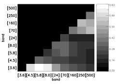
Figure 13: Determining the best color for recovering the fraction of dust in a smooth distribution in the envelope. Using the criterion described in §3.5, the best color for recovering the percentage of dust that is smooth was found to be [$3.6$]-[$5.8$]. However, as shown in Figure 16, even this ‘best’ color cannot be used to discriminate between the average values.

Figure 14: Determining the best color for recovering the R_out ratio. The best discriminator found for R_out, which also well separates and R_in/R_out ratios, is [$8.0$]-[$24$], and is shown in Figure 17.

Figure 15: The [$70$]-[$160$] color that can best be used to recover the SFE value. The diamonds are the average values over the entire dataset, and the error bars represent the one-$\sigma$ errors at each SFE value.

Figure 16: The [$3.6$]-[$5.8$] color that was found to best recover the fraction of dust that is smoothly distributed in the envelope. Given the 1-$\sigma$ error bars for the smoothest models (i.e. there is such a great diversity in this color due to the input parameters) it is only possible to separate the smooth from the clumpy models in a statistical sample where the standard deviation in the color could be measured.

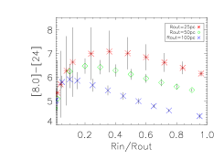
Figure 17: For envelopes with R_in/R${}_{out}\gtrsim 0.4$ the [$8.0$]-[$24$] color can be used to determine both the R_out value, because they are well separated from each other, and the R_in/R_out ratio.

4 COMPARISONS TO OBSERVATIONS

In the Milky Way, individual embedded massive stars are surrounded by what have been identified as “Ultracompact Hii Regions” (UCHiis), and it is hypothesized that the constituent massive stars in embedded SSCs will also be surrounded by UCHii regions. For this reason we compare our models to a sample of resolved embedded massive stars in order to test whether our models have reproduced, to first order, the necessary features of embedded massive stars. The sample is an IRAS sample studied in Wood & Churchwell (1989), in which it was found that 60% of the brightest IRAS sources ($>10^{4}$ Jy at 100µm) in the color range of their galactic survey are UCHii regions. Wood & Churchwell (1989) also found that galactic UCHii regions strictly obey a set of color criteria in the infrared with $log(F_{60\micron}/F_{12\micron})>1.30$ and $log(F_{25\micron}/F_{12\micron})>0.57$, while very few other types of objects had IRAS colors fitting these criteria. Therefore, these color criteria appear to be relatively robust for identifying UCHii regions, and we might expect natal SSCs to obey these criteria as well.

We have convolved our model results with the IRAS filter profiles, and Figure 18 shows the IRAS colors from a subset of our models compared to field objects (plus signs) and UCHii regions (diamonds) from the Kurtz, Churchwell, & Wood (1994) survey (which includes the Wood & Churchwell (1989) sample). In this figure, we focus on only the family of models with a 10% stellar mass component and a relative fraction of clumpy dust of 90%, although the other model families have IRAS colors that are included in the range represented by the models shown. Models with R${}_{out}=25$ pc are shown as red points, R${}_{out}=50$ pc as green points, and R${}_{out}=100$ pc as purple points. The values of R_in used are those shown in Table 1, and all sight-lines are shown for each set of model parameters, which produces additional scatter.

There is good agreement between our models and the UCHiis sample shown in Figure 18. There are a few of points to lower left and upper right that are not traced by our models. The lower left points have very hot dust in the inner portions of their envelopes, and might be modeled with a smaller R_in value that puts the hot dust closer to the heating source. The points to upper right seem to be an extension of the basic trend of increasing R_in. It is therefore possible that we could reproduce these UCHiis if we simply assumed a lower mass cutoff to our cluster which would lower the UV flux incident on the inner envelope.

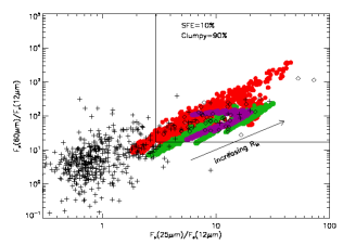
Figure 18: The IRAS colors from a subset of our models assuming 10% SFE and clumpy fraction = 0.9 compared to field objects (plus signs) and UCHii regions (diamonds) from the Kurtz, Churchwell, & Wood (1994) survey. Models with R${}_{\rm out}=25$ pc are shown as red points, R${}_{\rm out}=50$ pc as green points, and R${}_{\rm out}=100$ pc as purple points. The values of R_in used are those shown in Table 1, and all sight lines are shown for each set of model parameters.

5 KNOWN LIMITATIONS

Here we discuss some of the limitations of the models as a guide for future improvements.

($1$) The models assume that the central star cluster is a point source. While optical measurements have discovered half-light radii of super star clusters of $1.7$pc on average (de Marchi et al., 1997), which is significantly smaller than the assumed outer envelope radii, it is nevertheless more realistic to place several ultracompact Hii regions at the center of the envelope (see Figure 1). The intracluster dust would be heated at early evolutionary stages if multiple, smaller clusters were used, creating a hotter dust component than is seen with the current models.

($2$) Variations in metallicity have not been considered. For small changes in metallicity (i.e. down to half or third solar metallicity), we expect the dust-to-gas ratio to scale with metallicity. However, more extreme environments, like blue compact dwarf galaxies, where metallicities are often much lower than this, show dust in excess to what is expected from their metallicity alone (T. X. Thuan, private communication). Accounting for very low metallicities is therefore a complicated issue that is probably best handled on an individual basis.

($3$) The evolutionary sequences presented in this paper do not allow the central star cluster to evolve. As described in §2.5, the time between cluster formation and the dispersal of the embedding envelope is short, on the order of $~{}3-4$ Myr. However, the dispersal rate is not well known, so we have not made any attempt to place time stamps on the evolutionary sequence presented here. Hydrodynamical models are needed to answer this problem, and several hydrodynamical and semi-analytical studies of super star clusters already exist (e.g. Tenorio-Tagle et al., 2005, 2007; Wünsch et al., 2007, 2008). The rate at which the envelope is dispersed could potentially be answered by similar studies of a super star cluster’s embedded phase.

($4$) This work has concentrated solely on the dust emission and absorption in embedded super star clusters. Inclusion of nebular line emission in the model spectra could be useful if line diagnostics could be identified that break the model degeneracies.

($5$) The models do not include an interstellar radiation field (ISRF) incident on the outside of the dusty envelope. An ISRF would heat the dust on the outside of the envelope and provide an additional component to the starlight visible in the UV/optical/near-IR regime. This could affect the [$3.6$]-[$5.8$] color used to distinguish between different fractions of clumpy dust. The heating of the outer envelope could affect the far-IR fluxes as well.

6 SUMMARY

We present SEDs and colors of embedded SSCs created using spherical three-dimensional models. By varying the input parameters according to a series of evolutionary sequences, we have created a suite of models that can be used to constrain the evolutionary state of an embedded super star cluster. The main conclusions of the study are:

($1$) A hierarchically clumped medium is suitable for recreating the porous environments observed around embedded super star clusters (e.g. Johnson et al., 2009);

($2$) The infrared luminosity derived from a single sightline observation of a clumpy envelope can be wrong by as much as a factor of two from the true value;

($3$) The infrared SED also varies with sightline in these clumpy models, which has an impact on the near- and mid-infrared colors and magnitudes, the strength of the observed silicate features, and the dust continuum measured at these wavelengths;

($4$) For the smooth dust distribution models, the evolutionary sequences that begin with mid-infrared obscure envelopes (A${}_{V}\gtrsim 50$) are marked by a gradual decline in the silicate absorption features at $9.8$ and $17$µm  and a corresponding increase in the visual and ultraviolet flux as the cluster envelope evolves. Those sequences that begin with infrared-transparent envelopes (A${}_{V}<50$) instead have a predominant hot dust component and silicates in emission at early stages that eventually both fade away as the inner envelope radius moves outward. The clumpy envelope acts to confuse these general trends, making it harder to determine envelope properties.

($5$) Several diagnostic colors were found to constrain the envelope properties. The Spitzer MIPS [$70$]-[$160$] color is found to be a good diagnostic of the star formation efficiency, particularly at separating very low and high values (such as $5$% and $50$%) from more moderate values (between $10$% and $25$%). The [$3.6$]-[$5.8$] color can be used to determine the fraction of clumpy dust in the envelope for large samples of embedded super star clusters, but not for individual sources (see §3.5 for details). In order to determine the R_in and R_out values, the [$8.0$]-[$24$] color can be used for R_in/R${}_{out}\gtrsim 0.4$. Below this value the data is degenerate for all colors.

($6$) The model IRAS colors trace the same area of color space as ultracompact Hii regions, the Galactic analogues to extragalactic embedded super star clusters, suggesting that the models will also be useful when data of resolved, embedded super star clusters become available.

Table 1: The geometric sequences

R${}_{\rm out}=25$pc	R${}_{\rm out}=50$pc	R${}_{\rm out}=100$pc
Rin	Rin	Rin
0.1pc	0.1pc	0.1pc
0.5pc	0.5pc	1.0pc
1.0pc	1.0pc	5.0pc
2.0pc	5.0pc	10pc
3.0pc	10pc	15pc
6.0pc	15pc	25pc
9.0pc	20pc	35pc
12pc	25pc	45pc
15pc	30pc	55pc
18pc	35pc	65pc
21pc	40pc	75pc
24pc	45pc	95pc

Note. — Each sequence is run using clumpy dust fractions of 0.0, 0.1, 0.5, 0.9, and 0.99, and SFEs of 5%, 10%, 15%, 25%, and 50%, resulting in a total of 900 models. Stellar cluster mass of $10^{6}M_{\odot}$, source luminosity $\sim 1.6\times 10^{9}L_{\odot}$, Salpeter IMF $1-100M_{\odot}$, age 1 Myr, $Z_{\odot}$.

Table 2: A table of average A_V values and ranges for the R${}_{in}=0.1$pc models

SFE(%)	Rout	Smooth	$10$% clumpy	$50$% clumpy	$90$% clumpy	$99$% clumpy
5	25	490	474 (441-569)	411 (245-885)	348 (49.1-1200)	334 (4.92-1270)
5	50	123	119 (111-143)	103 (61.4-221)	87.0 (12.3-300)	83.4 (1.24-318)
5	100	30.8	29.8 (27.6-35.7)	25.8 (15.4-55.4)	21.8 (3.09-75.1)	20.9 (0.310-79.5)
10	25	232	225 (209-270)	195 (116-419)	165 (23.2-569)	158 (2.34-603)
10	50	58.2	56.3 (52.4-67.5)	48.8 (29.1-105)	41.2 (5.83-142)	39.5 (0.587-151)
10	100	14.6	14.1 (13.1-16.9)	12.2 (7.30-26.2)	10.3 (1.47-35.6)	9.88 (0.147-37.7)
15	25	146	142 (132-170)	123 (73.2-264)	104 (14.6-358)	99.5 (1.48-379)
15	50	36.7	35.5 (33.0-42.5)	30.7 (18.3-66.1)	26.0 (3.68-89.6)	24.9 (0.369-94.8)
15	100	9.18	8.88 (8.27-10.7)	7.69 (4.60-16.5)	6.50 (0.925-22.4)	6.23 (0.0925-23.7)
25	25	77.5	75.0 (69.7-89.9)	64.9 (38.7-140)	54.9 (7.76-190)	52.7 (0.781-201)
25	50	19.4	18.8 (17.5-22.5)	16.3 (9.71-35.0)	13.7 (1.95-47.4)	13.2 (0.196-50.2)
25	100	4.87	4.71 (4.38-5.65)	4.08 (2.44-8.76)	3.44 (0.490-11.9)	3.30 (0.0490-12.6)
50	25	25.8	25.0 (23.2-30.0)	21.7 (12.9-46.6)	18.3 (2.59-63.2)	17.6 (0.260-67.0)
50	50	6.48	6.27 (5.83-7.52)	5.43 (3.25-11.7)	4.59 (0.652-15.8)	4.40 (0.0652-16.7)
50	100	1.63	1.58 (1.47-1.89)	1.36 (0.816-2.93)	1.15 (0.163-3.96)	1.10 (0.0163-4.20)

Note. — The R_in value is $0.1$pc for all of these values. The range in A_V values depending on sightline are in parentheses for the clumpy models, with the average values shown first.

References

- Ashman & Zepf (2001) Ashman, K. M. & Zepf, S. E. 2001, AJ, 122, 1888
- Beck et al. (2002) Beck, S.C., Turner, J. L., Langland-Shula, L. E., Meier, D. S., Crosthwaite, L. P., Gorjian, V. 2002, AJ, 124, 251
- Bonnell et al. (2010) Bonnell, I. A., Smith, R. J., Clark, P. C., & Bate, M. R. 2010, MNRAS, in press. arXiv:1009.1152.
- Bosch et al. (2009) Bosch, G., Terlevich, E., & Terlevich, R. 2009, AJ, 137, 3437.
- Brogan et al. (2010) Brogan, C., Johnson, K., & Darling, J. 2010, ApJ, 716, 51.
- Cardelli et al. (1989) Cardelli, J. A., Clayton, G. C., & Mathis, J. S. 1989, ApJ, 345, 245
- Clark et al. (2005) Clark, J. S., Negueruela, I., Crowther, P. A., & Goodwin, S. P. 2005, A&A, 434, 949.
- Chakrabarti & Whitney (2009) Chakrabarti, S. & Whitney, B. A. 2009, ApJ, 690, 1432
- Conti & Vacca (1994) Conti, P. S., & Vacca, W. D. 1994, ApJ, 423, L97
- Cornette & Shanks (1992) Cornette, W. M. & Shanks, J. G. 1992 Applied Optics, 31, 3152
- de Marchi et al. (1997) de Marchi, G., Clampin, M., Greggio, L., Leitherer, C., Nota, A., & Tosi, M. 1997, ApJ, 479, L27.
- Draine et al. (2007) Draine, B. T.,Dale, D. A., Bendo, G., Gordon, K. D., Smith, J. D. T., Armus, L., Engelbracht, C. W., Helou, G., Kennicutt, R. C., Li, A., Roussel, H., Walter, F., Calzetti, D., Moustakas, J., Murphy, E. J., Rieke, G. H., Bot, C., Hollenbach, D. J., Sheth, K. & Teplitz, H. I. 2007, ApJ, 663, 866
- Draine & Li (2007) Draine, B. T., & Li, A. 2007, ApJ, 657, 810
- Eldridge & Relaño (2010) Eldridge, J. J., & Relaño, M. 2010, MNRAS, submitted. arXiv:1009.1871.
- Elmegreen (1997) Elmegreen, B. G. 1997, ApJ, 477, 196
- Elmegreen & Efremov (1997) Elmegreen, B. G., & Efremov, Y. N. 1997, ApJ, 480, 235.
- Fazio et el. (2004) Fazio, G. G. et al. 2004, ApJS, 154, 10
- Galliano et al. (2008) Galliano, F., Madden, S. C., Tielens, A. G. G. M., Peeters, E., & Jones, A. P. 2008, ApJ, 679, 310.
- Holtzman et al. (1992) Holtzman, J. A., Faber, S. M., Shaya, E. J., Lauer, T. R., Groth, E. J., Hunter, D. A., Baum, W. A., Ewald, S. P., Hester, J. J., Light, R. M., Lynds, C. R., O’Neil, E. J., & Westphal, J. A. 1992, AJ, 103, 691
- Hunt et al. (2005) Hunt, L., Bianchi, S., & Maiolino, R. 2005, A&A, 434, 849
- Indebetouw et al. (2006) Indebetouw, R., Whitney, B. A., Johnson, K. E, & Wood, K. 2006, ApJ, 636, 362
- Johnson et al. (1999) Johnson, K. E., Vacca, W. D., Leitherer, C., Conti, P. S., & Lipsky, S. J. 1999, AJ, 117, 1708
- Johnson et al. (2000) Johnson, K. E., Leitherer, C., Vacca, W. D., & Conti, P. S. 2000, AJ, 120, 1273
- Johnson et al. (2003) Johnson, K. E., Indebetouw, R., & Pisano, D. J. 2003, AJ, 126, 101
- Johnson & Kobulnicky (2003) Johnson, K. E. & Kobulnicky, H. A. 2003, ApJ, 597, 923
- Johnson et al. (2009) Johnson, K. E., Hunt, L. K., Reines, A. E. 2009, AJ, 137, 3788
- Kim et al. (1994) Kim, S.-H., Martin, P. G., & Hendry, P. D. 1993, ApJ, 422, 164
- Kim et al. (2008) Kim, Y., Rieke, G. H., Krause, O., Misselt, K., Indebetouw, R., & Johnson, K. E. 2008, ApJ, 678, 287.
- Kobulnicky & Johnson (1999) Kobulnicky, H. A. & Johnson, K. E. 1999, ApJ, 527, 154
- Kurtz, Churchwell, & Wood (1994) Kurtz, S., Churchwell, E., Wood, D. O. S. 1994, ApJS, 91, 659
- Laor & Draine (1993) Laor, A. & Draine, B. T. 1993, ApJ, 402, 441
- Leitherer et al. (1999) Leitherer, C., Schaerer, D., Goldader, J. D., González Delgado, R. M., Robert, C., Kune, D. F., de Mello, D. F., Devost, D., Heckman, T. M. 1999, ApJS, 123, 3
- Lucy (1999) Lucy, L. B. 1999, A&A, 344, 282
- Murray et al. (2010) Murray, N., Quataert, E., & Thompson, T. A. 2010, ApJ, 709, 191.
- Murray et al. (2010) Murray, N., Menard, B., & Thompson, T. A. 2010, ApJ, submitted. arXiv:1005.4419
- O’Connell et al. (1994) O’Connell, R. W., Gallagher, J. S., & Hunter, D. A. 1994, 433, 65
- Reines et al. (2008) Reines, A. E., Johnson, K. E., & Hunt, L. K. 2008, AJ, 135, 2222
- Rieke et al. (2004) Rieke, G., et al. 2004, ApJS, 154, 25.
- Robinson & Maldoni (2010) Robinson, G., & Maldoni, M. M. 2010, MNRAS, 408, 1956.
- Salpeter (1955) Salpeter, E. E. 1955, ApJ, 121, 161
- Sauvage & Plante (2003) Sauvage, M., & Plante, S. 2003, Ap&SS, 284, 941
- Schweizer et al. (1996) Schweizer, F., Miller, B. Y., Whitmore, B. C., & Fall, S. M. 1996, AJ, 112, 1839
- Shioya et al. (2001) Shioya, Y., Taniguchi, Y., & Trentham, N. 2001, MNRAS, 321, 11.
- Sonneborn (2008) Sonneborn, G. 2008, IAU Symposium 250, 491
- Tacconi-Garman et al. (1996) Tacconi-Garman, L. E., Sternberg, A., & Eckart, A. 1996, AJ, 112, 918.
- Tenorio-Tagle et al. (2005) Tenorio-Tagle, G., Silich, S., Rodríguez-González, A., Muñoz-Tuñón, C. 2005, ApJ, 620, 217.
- Tenorio-Tagle et al. (2007) Tenorio-Tagle, G., Wünsch, R., Silich, S., Palous̆, J. 2007, ApJ, 658, 1196.
- Thuan et al. (2005) Thuan, T. X., Lecavelier des Etangs, A., & Izotov, Y. I. 2005, ApJ, 621, 269.
- Turner et al. (2000) Turner, J. L., Beck, S. C., & Ho, P. T. P. 2000, ApJ, 532, 109
- Vacca, Johnson, & Conti (2002) Vacca, W. D., Johnson, K. E., & Conti, P. S. 2002, AJ, 123, 772
- Verschuur (1995) Verschuur, G. L. 1995, Ap&SS, 227, 187
- Warren (1984) Warren, S. G. 1984, Appl. Opt., 23, 1206
- Whitmore (2002) Whitmore, B. C. 2002, in: A Decade of Hubble Space Telescope Science, M. Livio, K. Noll, M. Stiavelli, Eds. (Cambride Univ. Press, Cambridge, 2002), pp. 153-180
- Whitney et al. (2003) Whitney, B. A., Wood, K., Bjorkman, J. E., & Wolff, M. J. 2003, ApJ, 591, 1049
- Whittet et al. (2001) Whittet, D. C. B., Gerakines, P. A., Hough, J. H., & Shenoy, S. S. 2001, ApJ, 547, 872
- Wood & Churchwell (1989) Wood, D. O. S. & Churchwell, E. 1989, ApJ, 340, 265
- Wood et al. (2008) Wood, K., Whitney, B. A., Robitaille, T., & Draine, B. T. 2008, ApJ, 688, 1118
- Wünsch et al. (2007) Wünsch, R., Silich, S., Palous̆, J., Tenorio-Tagle, G. 2007, A&A, 471, 579.
- Wünsch et al. (2008) Wünsch, R., Teonorio-Tagle, G., Palous̆, J., & Silich, S. 2008, AJ, 135, 2222.