Generalized Belief Propagation for the
Noiseless Capacity and Information Rates of Run-Length Limited Constraints

Abstract

The performance of the generalized belief propagation algorithm to compute the noiseless capacity and mutual information rates of finite-size two-dimensional and three-dimensional run-length limited constraints is investigated. In both cases, the problem is reduced to estimating the partition function of graphical models with cycles. The partition function is then estimated using the region-based free energy approximation technique. For each constraint, a method is proposed to choose the basic regions and to construct the region graph which provides the graphical framework to run the generalized belief propagation algorithm. Simulation results for the noiseless capacity of different constraints as a function of the size of the channel are reported. In the cases that tight lower and upper bounds on the Shannon capacity exist, convergence to the Shannon capacity is discussed. For noisy constrained channels, simulation results are reported for mutual information rates as a function of signal-to-noise ratio.

I Introduction

Run-length limited (RLL) constraints are widely used in magnetic and optical recording systems. Such constraints reduce the effect of inter-symbol interference and help in timing control. In track-oriented storage systems constraints are defined in one dimension.

We say a binary one-dimensional (1-D) sequence satisfies the $(d,k)$-RLL constraint if the runs of $0$’s have length at most $k$ and the runs of $0$’s between successive $1$’s have length at least $d$. We suppose that $0\leq d<k\leq\infty$.

The Shannon capacity of a 1-D $(d,k)$-RLL constraint is defined as

$$C_{1D}^{(d,k)}\stackrel{{\scriptstyle\scriptscriptstyle\bigtriangleup}}{{=}}\lim_{m\to\infty}\frac{\log_{2}Z(m)}{m},$$ (1)

where $Z(m)$ denotes the number of binary 1-D sequences of length $m$ that satisfy the $(d,k)$-RLL constraint, see [1, 2].

With the rise in demand for larger storage in smaller size and with recent developments in page-oriented storage systems, such as holographic data storage, two-dimensional (2-D) constraints have become more of interest [3]. In these systems, data is organized on a surface and constraints are defined in two dimensions.

A 2-D binary array satisfies the $(d_{1},k_{1},d_{2},k_{2})$-RLL constraint if it satisfies a $(d_{1},k_{1})$-RLL constraint horizontally and a $(d_{2},k_{2})$-RLL constraint vertically. If a 2-D binary array satisfies a 1-D $(d,k)$-RLL constraint both horizontally and vertically, we simply say that it satisfies a 2-D $(d,k)$-RLL constraint.

Example: 2-D $(2,\infty)$-RLL constraint:

The 2-D $(2,\infty)$-RLL constraint is satisfied in the following 2-D binary array segment. In words, in every row and every column of the array there are at least two $0$’s between successive $1$’s; but the runs of $0$’s can be of any length (however, $1$’s can be diagonally adjacent).

$\ldots 0100100001001000100000100010\ldots$$\ldots 1000010000100010000100000100\ldots$$\ldots 0001000010000001000000010001\ldots$$\ldots 0100100100010000001000100000\ldots$

The Shannon capacity of a 2-D $(d_{1},k_{1},d_{2},k_{2})$-RLL constraint is defined as

$$C_{2D}^{(d_{1},k_{1},d_{2},k_{2})}\stackrel{{\scriptstyle\scriptscriptstyle\bigtriangleup}}{{=}}\lim_{m,n\to\infty}\frac{\log_{2}Z(m,n)}{mn},$$ (2)

where $Z(m,n)$ denotes the number of 2-D binary arrays of size $m\times n$ that satisfy the $(d_{1},k_{1},d_{2},k_{2})$-RLL constraint.

Similarly, the Shannon capacity can be defined for higher dimensional constrained channels. For example, the Shannon capacity in three dimensions $C_{3D}^{(d_{1},k_{1},d_{2},k_{2},d_{3},k_{3})}$ depends on $Z(m,n,q)$, the number of three-dimensional (3-D) binary arrays of size $m\times n\times q$ that satisfy a $(d_{1},k_{1},d_{2},k_{2},d_{3},k_{3})$-RLL constraint.

The noiseless capacity of a constrained channel is an important quantity that provides an upper bound to the information rate of any encoder that maps arbitrary binary input into binary data that satisfies a given constraint. There are a number of techniques to compute the 1-D Shannon capacity (for example combinatorial or algebraic approaches) [1]. In contrast to the 1-D capacity, except for a few cases, exact values of two and higher dimensional (positive) Shannon capacities are not known, see [4, 5, 7, 6, 8, 9].

For noisy 1-D constrained channels, simulation-based techniques proposed in [16, 17] can be used to compute mutual information rates. However, computing mutual information rates of noisy 2-D RLL constraints has been an unsolved problem.

In this paper, the goal is to apply the generalized belief propagation (GBP) algorithm [10] for the above-mentioned problems, namely, to compute an estimate of the capacity of noiseless 2-D and 3-D RLL constrained channels and mutual information rates of noisy 2-D constrained channels. For both problems GBP turns out to yield very good approximate results.

Preliminary versions of the material of this paper have appeared in [11] and [12]. In [11], we applied GBP to compute the noiseless capacity of 2-D and 3-D RLL constrained channels. In [12], GBP was applied to compute mutual information rates of a 2-D $(1,\infty)$-RLL constrained channel with relatively small size and only at high signal-to-noise ratio (SNR). In this paper, we show that both problems reduce to estimating the partition function of graphical models with cycles. We then apply GBP to both problems and consider new constraints and larger sizes of grid.

Our main motivations for this research were the successful application of GBP for information rates of 2-D finite-state channels with memory in [13], Kikuchi approximation for decoding of LDPC codes and partial-response channels in [14], and tree-based Gibbs sampling for the noiseless capacity and information rates of 2-D constrained channels in [15, 12].

The outline of the paper is as follows. In Section II, we consider the problem of computing the partition function and discuss how this problem is related to computing the noiseless capacity and information rates of constrained channels. Region graphs, GBP, and region-based free energy are outlined in Section III. Section IV discusses the capacity of noiseless 2-D constraints. Numerical values and simulation results for the capacity of noiseless 2-D and 3-D RLL constraints are reported in Section IV-A. In Section V, we apply GBP to compute mutual information rates of noisy 2-D RLL constraints and report numerical experiments for mutual information rates in Section V-A.

II Problem Set-up

Consider a 2-D channel of size $N=m\times m$ with a set of $\textbf{X}=\{X_{1},X_{2},\ldots,X_{N}\}$ random variables. Let $x_{i}$ denote a realization of $X_{i}$ and let x denote $\{x_{1},x_{2},\ldots,x_{N}\}$. We assume that each $X_{i}$ takes values in a finite set $\mathcal{X}_{i}$. Also let $\mathcal{X}$ be the Cartesian product $\mathcal{X}\stackrel{{\scriptstyle\scriptscriptstyle\bigtriangleup}}{{=}}\mathcal{X}_{1}\times\mathcal{X}_{2}\times\ldots\times\mathcal{X}_{N}$.

In constrained channels, not all sequences of symbols from the channel alphabet $\mathcal{X}$ are admissible. Let $\mathcal{S}_{\textbf{X}}\subset\mathcal{X}$ be the set of admissible input sequences. We define the indicator function

$$f(\textbf{x})\stackrel{{\scriptstyle\scriptscriptstyle\bigtriangleup}}{{=}}\left\{\begin{array}[]{rl}1,&\textbf{x}\in\mathcal{S}_{\textbf{X}}\\ 0,&\textbf{x}\notin\mathcal{S}_{\textbf{X}}\end{array}\right.$$ (3)

The partition function $Z$ is defined as

$$Z\stackrel{{\scriptstyle\scriptscriptstyle\bigtriangleup}}{{=}}\sum_{\textbf{x}\in\mathcal{X}}f(\textbf{x}).$$ (4)

With the above definitions, $Z=|\mathcal{S}_{\textbf{X}}|$ is the number of sequences that satisfy a given constraint. Therefore, computing the capacity of constrained channels as expressed in (2), is closely related to computing the partition function as in (4).

Also note that with the above definitions

$$p(\textbf{x})=\frac{f(\textbf{x})}{Z}$$ (5)

is a probability mass function on $\mathcal{X}$.

For a noisy 2-D channel, let X be the input and $\textbf{Y}=\{Y_{1},Y_{2},\ldots,Y_{N}\}$ be the output of the channel. The mutual information rate is

$$\frac{1}{N}I(\textbf{X};\textbf{Y})=\frac{1}{N}\big{(}H(\textbf{Y})-H(\textbf{Y}|\textbf{X})\big{)}.$$ (6)

Let us suppose that $H(\textbf{Y}|\textbf{X})$ is analytically available. In this case, the problem of estimating the mutual information rate reduces to estimating the entropy of the channel output, which is

$$H(\textbf{Y})=-\operatorname{E}\big{[}\log p(\textbf{Y})\big{]}.$$ (7)

As in [16], we can approximate the expectation in (7) by drawing $L$ samples $\textbf{y}^{(1)},\textbf{y}^{(2)},\ldots,\textbf{y}^{(L)}$ according to $p(\textbf{y})$ and use the empirical average as

$$H(\textbf{Y})\approx-\frac{1}{L}\sum_{\ell=1}^{L}\log(p(\textbf{y}^{(\ell)})).$$ (8)

Therefore, the problem of estimating the mutual information rate reduces to computing $p(\textbf{y}^{(\ell)})$ for $\ell=1,2,\ldots,L$.

We will compute $p(\textbf{y}^{(\ell)})$ based on

$$p(\textbf{y}^{(\ell)})=\sum_{\textbf{x}\in\mathcal{X}}p(\textbf{x})p(\textbf{y}^{(\ell)}|\textbf{x}),$$ (9)

which for a fixed $\textbf{y}^{(\ell)}$ has also the form (4) and therefore requires the computation of a partition function.

RLL constraints impose restrictions on the values of variables that can be verified locally. For example, in a 2-D $(1,\infty)$-RLL constraint no two (horizontally or vertically) adjacent variables can both have the value $1$. The indicator function of this constraint factors into a product of kernels of the form

$$\kappa_{a}(x_{i},x_{j})=\left\{\begin{array}[]{ll}0,&\text{if $x_{i}=x_{j}=1$}\\ 1,&\text{else,}\end{array}\right.$$ (10)

with one such kernel for each adjacent pair $(x_{i},x_{j})$.

The factorization with kernels as in (10) can be represented with a graphical model. In this paper, we focus on graphical models defined in terms of Forney factor graphs. Fig. 1 shows the Forney factor graph of a 2-D $(1,\infty)$-RLL constraint where the boxes labeled “$=$” are equality constraints [19]. (Fig. 1 may also be viewed as a factor graph as in [18] where the boxes labeled “$=$” are the variable nodes).

In general, we suppose that the indicator function $f(\textbf{x})$ of an RLL constraint factors into a product of non-negative local kernels each having some subset of x as arguments; i.e.

$$f(\textbf{x})=\prod_{a}f_{a}(\textbf{x}_{a}),$$ (11)

where $\textbf{x}_{a}$ is a subset of x and each kernel $f_{a}(\textbf{x}_{a})$ has elements of $\textbf{x}_{a}$ as arguments.

In this case, the partition function in (4) can be written as

$$Z=\sum_{\textbf{x}\in\mathcal{X}}\prod_{a}f_{a}(\textbf{x}_{a}).$$ (12)

If the factorization in (11) yields a cycle-free factor graph (with not too many states), the sum in (12), or equivalently the sum in (4), can be computed efficiently by the sum-product message passing algorithm [18]. However, for the examples we study in this paper, like the Forney factor graph of a 2-D $(1,\infty)$-RLL constraint in Fig. 1, factor graphs contain (many short) cycles. In such cases computing $Z$ requires a sum with an exponential number of terms and therefore we are interested in applying approximate methods.

Due to the presence of many short cycles in the factor graph representation of 2-D and 3-D RLL constraints, loopy belief propagation often fails to converge. As a result, we apply GBP to estimate $Z$, which then leads to estimating the noiseless capacity and mutual information rates of RLL constraints.

Figure 1: Forney factor graph for a 2-D $(1,\infty)$-RLL constraint.

III GBP and the region graph method

In statistical physics, $Z$ defined in (4) is known as the partition function and the Helmholtz free energy is defined as

$$F_{H}\stackrel{{\scriptstyle\scriptscriptstyle\bigtriangleup}}{{=}}-\ln(Z).$$ (13)

The partition function and the Helmholtz free energy are important quantities in statistical physics since they carry information about all thermodynamic properties of a system.

A number of techniques have been developed in statistical physics to approximate the free energy. The method that we apply in this paper is known as the region-based free energy approximation, in particular we use the cluster variation method to select a valid set of regions and counting numbers, see [10] and [20] for more details.

We start by introducing the region graph representation of our problem. Such a region graph will provide a graphical framework for GBP algorithm. For each RLL constraint, the size of the basic region is chosen based on the constraint parameters. For a 2-D $(d_{1},k_{1},d_{2},k_{2})$-RLL constraint with finite $k_{1}$ and $k_{2}$, the width and the height of the basic region is chosen as

$$W_{R} = k_{1}+1$$

$$H_{R} = k_{2}+1,$$

and for the infinite case, the size is chosen as

$$W_{R} = d_{1}+1$$

$$H_{R} = d_{2}+1.$$

Such a choice for the basic regions seems plausible since the validity of a given array can be determined by verifying the constraints in each region and sliding the basic regions along the rows and along the columns of the array. For a 2-D $(1,\infty)$-RLL constraint, Fig. 2 shows the basic regions and Fig. 3 shows the region graph and the counting numbers associated with each region.

After forming the region graph using the cluster variation method, we perform GBP on this graph by sending messages between the regions while performing exact computations inside each region.

We will need the region-based free energy to estimate the number of arrays that satisfy a given constraint. Therefore, we operate GBP on the corresponding region graph until convergence and use the obtained region beliefs $\{b_{R}({\bf x}_{R})\}$ to compute the region-based free energy $\hat{F}_{H}$ (as an estimate of $F_{H}$). The region-based free energy $\hat{F}_{H}$ can then be used to estimate the partition function $Z$ using (13). We compute $\hat{F}_{H}$ as

$$\hat{F}_{H}\!\!\! = \!\!\!\!\min_{\{b_{R}\}}F_{\mathcal{R}}(\{b_{R}({\bf x}_{R})\})$$ (14)

$$= \!\!\!\!\!\sum_{R\in\mathcal{R}}\!\!\!c_{R}\!\sum_{{\bf x}_{R}}b_{R}({\bf x}_{R})\Big{(}\!\ln b_{R}({\bf x}_{R})-\ln\!\!\!\prod_{a\in A_{R}}\!\!f_{a}({\bf x}_{a})\!\Big{)}$$

Here $\mathcal{R}$ denotes the set of all regions, $c_{R}$ is the counting number, ${\bf x}_{R}$ stands for the set of variables in region $R$, and $A_{R}$ is the set of factors in region $R$. See Fig. 3.

Figure 2: Basic region of size $2\times 2$ for a 2-D $(1,\infty)$-RLL constraint.

Figure 3: The region graph for Forney factor graph in Fig. 2.

IV Capacity of Noiseless 2-D RLL Constraints

For a 2-D RLL constrained channel of width $m$ and of size $N=m\times m$, we run GBP on the corresponding region graph to compute $\hat{F}_{H}$ and an estimate of $Z$. We can then compute

$$C(m,m)=\frac{\log_{2}Z(m,m)}{m\times m},$$ (15)

where $Z(m,m)$ denotes the number of 2-D binary arrays of size $m\times m$ that satisfy the constraint.

In our numerical experiments in Section IV-A, for different RLL constraints we show convergence of $C(m,m)$ to the Shannon capacity as $m$ increases.

For example, let us consider a 2-D $(1,\infty)$-RLL constraint with corresponding Forney factor graph in Fig. 1. For this constraint, we chose basic regions with size $2\times 2$ in a sliding window manner over the factor graph, see Fig. 2. Starting from such basic regions, we applied the cluster variation method on the factor graph in Fig. 2 to obtain the corresponding region graph depicted in Fig. 3. The counting numbers $\{c_{R}\}$ are shown next to each region.

Figure 4: Estimated capacity (in bits per symbol) vs. channel width $m$ for a 2-D $(1,\infty)$-RLL constraint. The horizontal dotted line shows the Shannon capacity for this channel as in (16).

Figure 5: Estimated capacities (in bits per symbol) vs. channel width $m$ for a class of 2-D $(1,\infty,d,\infty)$-RLL constraints with $d=(1,2,3,4)$.

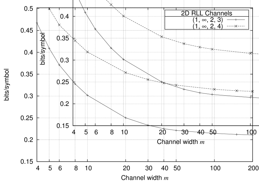
Figure 6: Estimated capacity (in bits per symbol) vs. channel width $m$ for a 2-D $(1,\infty,2,4)$-RLL and $(1,\infty,2,3)$-RLL constraints.

Figure 7: Estimated capacity (in bits per symbol) vs. channel width $m$ for a 2-D $(2,\infty)$-RLL constraint.

Figure 8: Estimated capacity (in bits per symbol) vs. channel width $m$ for a 3-D $(1,\infty)$-RLL constraint. The horizontal dotted lines show upper and lower bounds on the Shannon capacity for this channel as in (18).

IV-A Numerical Experiments

Here we present the numerical results of applying GBP to estimate the finite-sized noiseless capacity of RLL constraints.

Tight lower and upper bounds were given for the Shannon capacity of a 2-D $(1,\infty)$-RLL constraint in [4]. The bounds were further improved in [22] and [23], now known to nine decimal digits.

$$0.5878911617...\leq C_{2D}^{(1,\infty)}\leq 0.5878911618...$$ (16)

For this constraint, Fig. 5 shows $C(m,m)$ defined in (15) versus the channel width $m$ over the interval $[2,300]$. The estimation was performed using the parent-to-child and two-way GBP algorithms. The two algorithms give almost identical results. The horizontal line in Fig. 5 shows the Shannon capacity for this channel in (16). For a channel of width $300$, the estimated noiseless capacity is about $0.5884$.

Shown in Fig. 5 are plots of $C(m,m)$ for 2-D $(1,\infty,d,\infty)$-RLL constraints with $d=(1,2,3,4)$ from top to bottom, versus the channel width $m$ over the interval $[2,200]$. Fig. 7 shows the plots of $C(m,m)$ for 2-D $(1,\infty,2,4)$-RLL and $(1,\infty,2,3)$-RLL constraints versus $m$ over the interval $[4,200]$. From our simulation results, for a channel of width $200$ the estimated noiseless capacities for 2-D $(1,\infty,d,\infty)$-RLL constraints with $d=(2,3,4)$ are about $(0.4994,0.4346,0.3864)$ and the estimated noiseless capacities for 2-D $(1,\infty,2,4)$-RLL and $(1,\infty,2,3)$-RLL are about $(0.3106,0.2109)$. To the best of our knowledge, no theoretical upper or lower bounds exist for these constraints. All plots are obtained using the parent-to-child algorithm. Note that 2-D $(1,\infty,1,\infty)$-RLL plot in Fig. 5 is the same as the plot in Fig. 5.

Also shown in Fig. 7 is the plot of $C(m,m)$ for a 2-D $(2,\infty)$-RLL constraint versus $m$ over the interval $[3,400]$. For a channel of width $400$, the estimated noiseless capacity is about $0.4462$. Best known lower and upper bounds for the Shannon capacity of a 2-D $(2,\infty)$-RLL constraint are given in [8] and [9] respectively, as

$$0.4453\leq C_{2D}^{(2,\infty)}\leq 0.4457$$ (17)

Our proposed method can be generalized to compute the noiseless capacity of 3-D and higher dimensional RLL constraints. For a 3-D $(1,\infty)$-RLL constraint the following lower and upper bounds were introduced in [23]

$$0.5225017418...\leq C_{3D}^{(1,\infty)}\leq 0.5268808478...$$ (18)

Fig. 8 shows the noiseless capacity estimates of a 3-D $(1,\infty)$-RLL constraint, obtained using the parent-to-child algorithm, versus the channel width $m$. The horizontal dotted lines show the upper and lower bounds for the Shannon capacity. For a channel of width $m=40$ the GBP estimated capacity is about $0.5267$ which falls within these bounds.

Simulation results and numerical values for the noiseless capacity of many other 2-D RLL constraints are reported in [21].

IV-B Bounds for the Shannon Capacity

For any finite $m$, it is possible to compute lower and upper bounds on the Shannon (infinite-size) capacity using $C(m,m)$ the capacity of a 2-D RLL constrained channel of width $m$.

For example, consider a 2-D $(1,\infty)$-RLL constraint with local kernels as in (10). From tiling the whole plane with $m\times m$ squares, it is clear that $C(m,m)$ is an upper bound for the Shannon capacity $C_{2D}^{(1,\infty)}$. On the other hand, by tiling the plane with $m\times m$ squares separated by all-zero guard rows and all-zero guard columns, we obtain $(\frac{m}{m+1})^{2}C(m,m)\leq C_{2D}^{(1,\infty)}$.

From Fig. 5, the estimated capacity at $m=300$ is about $C(300,300)=0.5884$, we thus obtain the following lower and upper bounds for the Shannon capacity

$$0.5844\leq C_{2D}^{(1,\infty)}\leq 0.5884.$$

Note that although GBP performs remarkably well for 2-D constrained channels, it is an approximate algorithm which yields approximations to the lower and upper bounds to the Shannon capacity. However in order to achieve a desired precision, the bounds could provide a criterion for choosing the value of $m$.

Figure 9: Extension of Fig. 1 to a Forney factor graph of $p(\textbf{x},\textbf{y})$ with $p(\textbf{y}|\textbf{x})$ as in (22).

V Information Rates of Noisy 2-D RLL Constraints

As explained in Section II, the problem of computing mutual information rates reduces to computing the output probability. Therefore, the remaining tasks are

1. Drawing input samples $\textbf{x}^{(1)},\textbf{x}^{(2)},\ldots,\textbf{x}^{(L)}$ from $\mathcal{S}_{\textbf{X}}$ according to $p(\textbf{x})$ and therefrom creating output samples $\textbf{y}^{(1)},\textbf{y}^{(2)},\ldots,\textbf{y}^{(L)}$.

2. Computing $p(\textbf{y}^{(\ell)})$ for each $\ell=1,2,\ldots,L$.

We will compute $p(\textbf{y}^{(\ell)})$ based on

$$p(\textbf{y}^{(\ell)})=\sum_{\textbf{x}\in\mathcal{S}_{\textbf{X}}}p(\textbf{x})p(\textbf{y}^{(\ell)}|\textbf{x}),$$ (19)

where $p(\textbf{x})$ is a probability mass function on $\mathcal{S}_{\textbf{X}}$.

Let us assume uniform distribution over the admissible channel input configurations. Therefore we have

$$p(\textbf{x}) = |\mathcal{S}_{\textbf{X}}|^{-1}$$ (20)

$$= 2^{-NC_{2D}},$$ (21)

we also assume the channel is memoryless and $p(\textbf{y}|\textbf{x})$ factors as

$$p(\textbf{y}|\textbf{x})=\prod_{i=1}^{N}p(y_{i}|x_{i}).$$ (22)

For such a noisy 2-D constrained channel, the corresponding Forney factor graph, as an extension of Fig. 1, is shown in Fig. 9.

Using (21) and (22), we can rewrite (19) as

$$p(\textbf{y}^{(\ell)}) = 2^{-NC_{2D}}\sum_{\textbf{x}\in\mathcal{S}_{\textbf{X}}}\prod_{i=1}^{N}p(y^{(\ell)}_{i}|x_{i}),$$ (23)

$$= 2^{-NC_{2D}}Z(\textbf{y}^{(\ell)}),$$ (24)

where $Z(\textbf{y}^{(\ell)})$ has the same form as the sum in (12).

The input samples $\textbf{x}^{(1)},\textbf{x}^{(2)},\ldots,\textbf{x}^{(L)}$ are generated as follows. We run GBP on Fig. 3 until convergence to compute the region beliefs $\{b_{R}(\textbf{x}_{R})\}$ at each region $R$. The region beliefs are GBP approximations to the corresponding marginals $\{p_{R}(\textbf{x}_{R})\}$. In our numerical experiments, each sample $\textbf{x}^{(\ell)}$ is then generated piecewise sequentially according to the beliefs $b_{R}(\textbf{x}_{R})$ in basic regions. For example, in the region graph of Fig. 3, after computing $b_{R}(x_{1},x_{2},x_{4},x_{5})$, sample $x_{1}$ is drawn according to $b_{R}(x_{1})$, sample $x_{2}$ is drawn according to $b_{R}(x_{2}|x_{1})$, etc. The input samples $\textbf{x}^{(1)},\textbf{x}^{(2)},\ldots,\textbf{x}^{(L)}$ are then used to create output $\textbf{y}^{(1)},\textbf{y}^{(2)},\ldots,\textbf{y}^{(L)}$ using (22).

The beliefs are directly proportional to the factor nodes involved in each region, which guarantees that the samples are drawn from $\mathcal{S}_{\textbf{X}}$. Moreover, since beliefs are good approximations to the marginal probabilities, one expects that the samples are drawn from a distribution close to $p(\textbf{x})$, see [10].

In order to compute $Z(\textbf{y}^{(\ell)})$, as in Section III, we start from the factor graph in Fig. 9 to build the region graph representing the problem and run GBP on this region graph. Finally, the estimated $p(\textbf{y}^{(1)}),p(\textbf{y}^{(2)}),\ldots,p(\textbf{y}^{(L)})$ are used to compute an estimate of $H(\textbf{Y})$ as in (8).

V-A Numerical Experiments

In our numerical experiments we consider $(1,\infty)$-RLL and $(2,\infty)$-RLL constrained channels with size $N=30\times 30$ and input alphabet $\mathcal{X}=\{-1,+1\}^{N}$.

Noise is assumed to be i.i.d.  zero mean Gaussian with variance $\sigma^{2}$ and independent of the input. We thus have

$$H(\textbf{Y}|\textbf{X})=\frac{N}{2}\log(2\pi e\sigma^{2}),$$ (25)

and $p(\textbf{y}|\textbf{x})$ in (22) has kernels of the form

$$p(y_{i}|x_{i})=\frac{1}{\sqrt{2\pi\sigma^{2}}}\exp\!\bigg{(}-\frac{1}{2\sigma^{2}}\Big{(}y_{i}-x_{i}\Big{)}^{2}\bigg{)}.$$ (26)

SNR is defined as

$$\text{SNR}\stackrel{{\scriptstyle\scriptscriptstyle\bigtriangleup}}{{=}}10\log_{10}\frac{1}{\sigma^{2}}$$ (27)

Shown in Fig. 11 is the estimated information rate vs. SNR over the interval $[-10,10]$ dB for a noisy 2-D $(1,\infty)$-RLL constraint. The horizontal dotted line shows the estimated noiseless capacity which can be read from Fig. 5 and is about $0.5943$ for this size of channel.

Illustrated in Fig. 11 is the estimated information rate vs. SNR over the interval $[-10,10]$ dB for a noisy 2-D $(2,\infty)$-RLL channel. The horizontal dotted line shows the estimated noiseless capacity which can be read from Fig. 7 and is about $0.4552$ for this size of channel.

The simulation results were obtained by averaging over $L=1000$ realizations of the channel output.

Simulation results and numerical values for mutual information rates of many other 2-D RLL constraints are reported in [21].

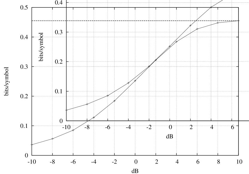
Figure 10: Estimated information rate (in bits per symbol) vs. SNR (in dB) for a $30\times 30$ channel with a $(1,\infty)$-RLL constraint and additive white Gaussian noise.

Figure 11: Estimated information rate (in bits per symbol) vs. SNR (in dB) for a $30\times 30$ channel with a $(2,\infty)$-RLL constraint and additive white Gaussian noise.

VI Concluding remarks

We proposed a GBP-based method to estimate the noiseless capacity and mutual information rates of RLL constraints in two and three dimensions. For noiseless RLL constraints, the method was applied to estimate the finite-size capacity of different constraints and to show convergence to the Shannon capacity as the size of the channel increases. In particular, the proposed method can be used to estimate the noiseless capacity of RLL constraints in the cases that the capacity is not known to a useful accuracy. The method was also applied to estimate mutual information rates of noisy RLL constraints with additive white Gaussian noise and with a uniform distribution over the admissible input configurations. Our simulation results show mutual information rates of different constraints as a function of SNR.

References

- [1] K. A. Schouhamer Immink, Codes for Mass Data Storage Systems. Eindhoven: Shannon Foundation Publishers, 2004.
- [2] C. E. Shannon, “A mathematical theory of communications,” Bell Sys. Tech. Journal, vol. 27, pp. 379–423, July 1948.
- [3] P. H. Siegel, “Information-theoretic limits of two-dimensional optical recording channels,” in Optical Data Storage (Proc. of SPIE, Vol. 6282, Eds. Ryuichi Katayama and Tuviah E. Schlesinger), Montreal, Quebec, Canada, April 2006.
- [4] N. J. Calkin and H.S. Wilf, ‘The number of independent sets in a grid graph,” SIAM J. Discr. Math., vol. 11, pp. 54–60, Feb. 1998.
- [5] S. Forchhammer and T.V. Laursen, “Entropy of bit-stuffing-induced measures for two-dimensional checkerboard constraints,” IEEE Trans. Inform. Theory, vol. 53, pp. 1537–1546, April 2007.
- [6] H. Ito, A. Kato, Z. Nagy, and K. Zeger, ‘Zero capacity region of multidimensional run length constraints,” The Electronic Journal of Combinatorics, vol. 6(1), 1999.
- [7] K. Kato and K. Zeger, ‘On the capacity of two-dimensional run-length constrained channels,” IEEE Trans. Inform. Theory, vol. 45, pp. 1527–1540, July 1999.
- [8] E. Ordentlich and R. M. Roth, “Approximate enumerative coding for 2-D constraints through ratios of matrix products,” Proc. 2009 IEEE Int. Symp. on Information Theory, Seoul, Korea, pp. 1050–1054.
- [9] I. Tal and R. M. Roth, “Concave programming upper bounds on the capacity of 2-D constraints,” IEEE Trans. Inform. Theory, vol. 57, pp. 381–391, Jan. 2011.
- [10] J. S. Yedidia, W. T. Freeman, and Y. Weiss. “Constructing free energy approximations and generalized belief propagation algorithms,” IEEE Trans. Inform. Theory, vol. 51, pp. 2282–2312, July 2005.
- [11] G. Sabato and M. Molkaraie, “Generalized belief propagation algorithm for the capacity of multi-dimensional run-length limited constraints,” Proc. 2010 IEEE Int. Symp. on Information Theory, Austin, USA, June 13–18, pp. 1213–1217.
- [12] M. Molkaraie and H.-A. Loeliger, “Estimating the information rate of noisy constrained 2-D channels,” Proc. 2010 IEEE Int. Symp. on Information Theory, Austin, USA, June 13–18, pp. 1678–1682.
- [13] O. Shental, N. Shental, S. Shamai (Shitz), I. Kanter, A. J. Weiss, and Y. Weiss, “Discrete-input two-dimensional Gaussian channels with memory: estimation and information rates via graphical models and statistical mechanics,” IEEE Trans. Inform. Theory, vol. 54, pp. 1500–1513, April 2008.
- [14] P. Pakzad and V. Anantharam, “Kikuchi approximation method for joint decoding of LDPC codes and partial-response channels,” IEEE Trans. Communications, vol. 54, pp. 1149–1153, July 2006.
- [15] H.-A. Loeliger and M. Molkaraie, “Estimating the partition function of 2-D fields and the capacity of constrained noiseless 2-D channels using tree-based Gibbs sampling,” Proc. 2009 IEEE Information Theory Workshop, Taormina, Italy, Oct. 11–16, pp. 228–232.
- [16] D. Arnold, H.-A. Loeliger, P. O. Vontobel, A. Kavčić, and W. Zeng, “Simulation-based computation of information rates for channels with memory,” IEEE Trans. Inform. Theory, vol. 52, no. 8, pp. 3498–3508, August 2006.
- [17] H. D. Pfister, J.-B. Soriaga, and P. H. Siegel, “On the achievable information rates of finite-state ISI channels,” in Proc. 2001 IEEE Globecom, San Antonio, USA, Nov. 25–29, pp. 2992–2996.
- [18] F. R. Kschischang, B. J. Frey, and H.-A. Loeliger, “Factor graphs and the sum-product algorithm,” IEEE Trans. Inform. Theory, vol. 47, pp. 498–519, Feb. 2001.
- [19] H.-A. Loeliger, “An introduction to factor graphs,” IEEE Signal Proc. Mag., Jan. 2004, pp. 28–41.
- [20] M. Welling, “On the choice of regions for generalized belief propagation,” Proc. 2004 conference on Uncertainty in artificial intelligence, Banff, Canada, pp. 585–592.
- [21] G. Sabato, Simulation-based techniques to study two-dimensional ISI channels and constrained systems. Master thesis, Dept. Inform. Techn. & Electr. Eng, ETH Zürich, Switzerland, 2009.
- [22] W. Weeks and R. E. Blahut, “The capacity and coding gain of certain checkerboard codes,” IEEE Trans. Inform. Theory, vol. 44, pp. 1193–1203, May 1998.
- [23] Z. Nagy and K. Zeger, ‘Capacity bounds for the three-dimensional run-length limited channels,” IEEE Trans. Inform. Theory, vol. 46, pp. 1030–1033, May 2000.