Atmospheric time constant with MASS and FADE

Abstract

The approximate nature of the adaptive-optics time constant measurements with MASS is examined. The calibration coefficient C derived from numerical simulations of polychromatic scintillation shows dependence on the height of the turbulence layer, wind speed, and seeing. The previously recommended value of C=1.27 is a good match to typical conditions, while C can vary from 0.6 to 1.6 in other circumstances. For two nights, MASS was compared with the time constant measured with adaptive optics, and the expected agreement was found. We show that the single-layer approximation used in some AO systems to derive the AO time constant can give wrong results. A better approach is to estimate it from the speed of focus variation (the FADE method). The analysis of the speed of scintillation developed recently by V. Kornilov will lead to more accurate measurements of the AO time constant with MASS.

1 Definitions and context

The adaptive optics atmospheric time constant $\tau_{0}$ depends on the wind speed and turbulence profiles. It is defined as

$$\tau_{0}=0.314r_{0}/\overline{V}_{5/3}=0.057\;\lambda_{0}^{6/5}\left[\int_{o}^{\infty}C_{n}^{2}(h)\;V^{5/3}(h)\;{\rm d}h\right]^{-3/5},$$ (1)

where $C_{n}^{2}(h)$ is the vertical profile of the refractive index structure constant, $V(h)$ is the vertical profile of the modulus of the wind speed, $h$ is the altitude above site. In the following we always assume that $\tau_{0}$ refers to the wavelength $\lambda_{0}=0.5$ $\mu$m and observations at zenith. As the correction for the zenith distance depends on the unknown wind direction, it is simply ignored [9].

The MASS instrument implements an approximate method [6] of estimating $\tau_{0}$ from the differential-exposure scintillation index, DESI. The $\sigma^{2}_{DESI}$ is computed for the smallest 2-cm MASS aperture as a differential index between 1 ms and 3 ms exposures. A formula

$$\tau_{MASS}=0.175\,{\rm ms}\;(\sigma^{2}_{DESI})^{-0.6}$$ (2)

has been suggested on the basis of limited data on real turbulence profiles. This formula is implemented in the standard MASS data processing

We found later by means of simulations that $\tau_{MASS}$ calculated from (2) needs a corrective coefficient around $C=1.27$ The true time constant could be derived from the MASS data by applying this correction and adding the contribution of the ground layer (GL) which is not sensed by MASS (but measured with MASS-DIMM). Therefore, the AO time constant is estimated by MASS-DIMM as

$$\tau_{0}^{-5/3}=(1.27\,\tau_{MASS})^{-5/3}+(0.057)^{-5/3}\lambda_{0}^{-2}\;V_{GL}^{5/3}\;(C_{n}^{2}{\rm d}h)_{GL}.$$ (3)

The intrinsic accuracy of such estimate was evaluated to be $\pm 20$% or better.

Travouillon et al. [9] have derived a somewhat different correction factor $C=1.73$ by calculating $\tau_{0}$ from the turbulence profile measured by MASS and using NCEP wind velocities. Even larger factors of 2.45 and 2.11 were determined in Ref. 7 by the same method. This prompted a re-investigation of this matter by doing new simulations and comparing with alternative techniques.

2 Numerical simulations

We simulate one phase screen at a given height $h$ and calculate the intensity at the ground by means of the program simatmpoly.pro. The intensity pattern is a weighted sum for several wavelengths. Here we approximate the spectral response of MASS by 4 wavelengths of [400,450,500,550] nm with weights [0.31, 0.885, 0.60, 0.27]. This should mimic the response of TMT MASS-DIMMs, as studied by Kornilov [4]. He found for these instruments effective wavelength 474 nm and the bandwidth 99 nm (response curve without.crv). For our 4-wavelength approximation, the effective wavelength and bandwidth are 470 nm and 116 nm, respectively. The simulation does not include the light-source spectrum, assuming it flat.

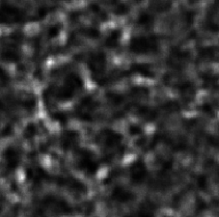
Figure 1: Fragment of the simulated scintillation pattern produced on the ground by a turbulent layer at 10 km with $0.5^{\prime\prime}$ seeing. The scintillation index is 0.27, the size of the fragment is 0.5 m.

The simulated intensity distributions (Fig. 1) are saved in a binary file. In the previous simulator they were used in a Monte-Carlo approach where the 2-cm MASS aperture was “dragged” through the intensity screen, while 1-ms and 3-ms exposure time was emulated by suitable blurring of the aperture in one direction and by 3x binning. Here we take a more direct approach and calculate DESI with the spatial filter

$$P(f_{x})={\rm sinc}(f_{x}b)-{\rm sinc}(3f_{x}b),$$ (4)

where $f_{x}$ is the component of spatial frequency, $b=Vt_{exp}$ is the blur in the x-direction caused by the wind speed $V$ during exposure time $t_{exp}=1$ ms and ${\rm sinc}(x)=\sin(\pi x)/(\pi x)$. The circular aperture of diameter $d$ implies the filter

$$A(f)=\frac{2J_{1}(\pi fd)}{\pi fd}.$$ (5)

The energy spectrum of the intensity is multiplied by the combined filter $(AP)^{2}$ and summed over all frequencies to get the DESI index. By omitting all filters, we obtain the raw scintillation index, by using only filter $A$ – the scintillation index in the 2-cm aperture. Results for a test case were compared with previous simulations and found to be in agreement, validating the code.

Considering that the calculation of intensity distribution is the most time-consuming task, we simulate the intensity screen for a given seeing and propagation distance and then calculate DESI and $\tau_{MASS}$ for a set of 12 wind speeds, from 10 m/s to 65 m/s, by changing only the filter $P$. The calculation is repeated for 3 distances to the layer, 5, 10, and 15 km, and for 5 values of seeing $\varepsilon$, from $0.3^{\prime\prime}$ to $1.5^{\prime\prime}$. Therefore we cover a wide range of conditions, with a varying degree of saturated scintillation. The largest scintillation index is 0.94 (layer at 15 km, seeing $1.5^{\prime\prime}$). In each case, the true time constant at $\lambda_{0}$ is known, $\tau_{0}=0.31r_{0}/V=0.31(0.101/\varepsilon)/V$. We determine the corrective coefficient $C=\tau_{0}/\tau_{MASS}$ for each case.

Figure 2: Correction factor $C$ as a function of the wind speed for a single turbulent layer at distance 5 km (left) and 10 km (right). The turbulence strength of the layer (seeing) is from $0.3^{\prime\prime}$ to $1.5^{\prime\prime}$. The dotted horizontal line shows $C=1.27$.

Figure 3: Left: Correction factor $C$ as a function of the wind speed for a single turbulent layer at distance 15 km. Right: all values of $\tau_{MASS}$ plotted against $\tau_{0}$, the dotted line corresponds to $C=1.27$.

This study clearly shows that estimates of $\tau_{0}$ from DESI are approximate and can be off by as much as two times. No single corrective coefficient $C$ can be derived, it varies from 0.6 to 1.6. For typical conditions ($V=30$ m/s, turbulence at 200 mb), $C=1.27$ appears to be a good choice.

3 Comparison of MASS with FADE

Any working AO system provides real-time data on turbulence from which the AO time constant can be derived. For example, the covariance of atmospheric defocus falls to 1/2 of its maximum for a time lag $t_{0.5}=0.30D/V$. It follows that $\tau_{0}=1.05t_{0.5}(r_{0}/D)$. A method of estimating $\tau_{0}$ from half-time correlation of Zernike aberrations has been proposed by Fusco et al. [1] and implemented in the NAOS at Paranal. It is valid for a single turbulent layer, but the authors argue that for several layers some “average” wind speed will result from $t_{0.5}$. This is not quite true, as we will see in a moment.

Theory [2, 8] shows that the temporal structure function (SF) of defocus $D_{4}(t)$ produced by a combination of several atmospheric layers has the form

$$D_{4}(t)\approx 1.94D^{5/3}\sum_{i}r_{0,i}^{-5/3}K_{4}(2V_{i}t/D,\epsilon)+N,$$ (6)

where $D$ is the telescope diameter, $\epsilon$ is the central obscuration ratio, $r_{0,i}$ and $V_{i}$ are the Fried parameters and wind speeds of the layers, $N$ is the term caused by the measurement noise. The function $K(x,y)$ is defined in Ref. 8. It has a quadratic initial part at $t\ll t_{0.5}$, where small focus changes are proportional to time. In this short-exposure regime, the speed of defocus variation is related to the integral of $V^{2}(h)C_{n}^{2}(h){\rm d}h$ – the 2-nd moment of the wind speed $\overline{V}_{2}$. It is rather close to the 5/3rd moment $\overline{V}_{5/3}$ used in the definition of $\tau_{0}$. The method to estimate $\tau_{0}$ from the speed of focus variation is called FADE (FAst DEfocus) [2, 8]. It is resumed by a simple formula

$$D_{4}(t)\approx 0.036(D/r_{0})^{-1/3}(t/\tau_{0})^{2}.$$ (7)

Figure 4: Left: example of the measured defocus SF (line) and its model by two layers (asterisks). The vertical axis in rad² at 500 nm wavelength. Right: SF of defocus for two layers with $1^{\prime\prime}$ and $0.4^{\prime\prime}$ seeing moving at 10 and 60 m/s, respectively. the dotted line shows half-saturation and corresponds to $t_{0.5}$.

Figure 4 shows the SF of defocus measured with the SOAR Adaptive Module (SAM) on October 2009. In this case $D=4.1$ m, $\epsilon=0.24$. Taking the wind speed of 50 m/s, we estimate $t_{0.5}\sim 25$ ms, or 6 loop cycles of SAM. Therefore, the temporal sampling of SAM (4.2 ms) is adequate for applying the FADE technique. By fitting the initial part of the SF with a two-layer model (6), we derive the defocus speed and $\tau_{0}$.

A simple test case presented in Fig. 4, right, shows why the half-time method can give wrong results. The $t_{0.5}=0.105$ s is essentially determined here by the strongest and slowest layer, leading to the estimate $\tau_{0}=2.39$ ms. The actual time constant $\tau_{0}=1.15$ ms is mostly produced by the weak and fast layer which makes the dominant contribution to the speed of defocus and to the shape of the initial (quadratic) SF. The error of the half-time method to estimate $\tau_{0}$ in this case is 2.1 times.

So far, the SAM data were collected and processed for two nights, August 31 and October 2, 2009 (hereafter nights 1 and 2). AO loop data were recorded several times during $\sim 12$ s. Atmospheric variations of defocus were derived from the signals of the corrector (DM), accounting for the frequency response of the closed AO loop. Voltages are transformed into Zernike coefficients in radians at $\lambda_{0}$. The variance of the low-order Zernike coefficients is used to estimate the Fried parameter $r_{0}$ (seeing).

Derivation of $\tau_{0}$ from the loop data involves few subtleties. First, we suppress all frequencies above 45 Hz because the data show focus vibration at 46 Hz (this low-pass filtering has little effect on the results, however). Second, the estimates depend on the maximum time lag used in the model-fitting. This length was varied from just 4 first points to 0.1 s and 0.4 s. With increasing lag, the estimates $\tau_{0,SAM}$ also become larger, see Table 1. The fitted models show that on night 1 there was a fast-moving layer.

Table 1: Average parameters from the FADE model fits

Parameter	Night 1			Night 2
	4pt	0.1s	0.3s	4pt	0.1s	0.3s
$\tau_{0,MASS}/\tau_{0,SAM}$	0.73	0.83	0.91	1.42	1.25	1.02
$\overline{V}$, m/s	30.5	36.6	27.6	24.6	27.8	19.0
$V_{layer2}$, m/s	-	63.9	47.1	-	64.9	32.8

The MASS-DIMM monitor at Cerro Pachón provided data for comparison with FADE. We used the ground wind speed and applied the formula (3) with $C=1.27$ to get $\tau_{0,MASS}$. The seeing on the night 1 was fast and bad, while the conditions on the night 2 (Fig. 5, right) were closer to typical, but only 4 hours were clear. Different structure of turbulence on these two nights leads to different systematics between MASS and FADE (Fig. 5, left). We cannot tell whether $C=1.27$ has to be increased or decreased, it is “about right”.

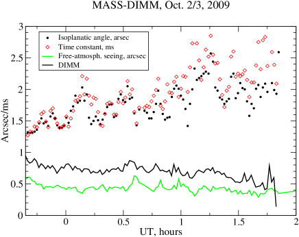
Figure 5: Left: Comparison of simultaneous $\tau_{0}$ from FADE (fitting 0.1 s) and MASS; the dashed line shows equality. Right: Summary plot of atmospheric conditions on October 2, 2009 from the Cerro Pachón MASS-DIMM site monitor.

4 Conclusions and further work

This study reveals, once again, the approximate nature of $\tau_{0}$ measurements from DESI implemented in the MASS software. Depending on the turbulence and wind profiles, the bias of MASS $\tau_{0}$ with the recommended correction factor $C=1.27$ can be either positive or negative. Attempts to find the best calibration coefficient are hampered by the above-mentioned dependence on conditions. Our simulations show that the correction factor $C=1.73$ found by Travouillon et al. [9] is too high. However, the simulations do not account for the spectrum of the star; if it moves the effective spectral response of MASS blue-wards, the correction factor will be larger.

Despite obvious shortcomings of the DESI method, it has a strong appeal, being a simple and no-cost addition to the MASS instrument. Considerable data on $\tau_{0}$ have been accumulated to date for many sites worldwide. We can do a better job on $\tau_{0}$ with MASS. Recent analysis by Kornilov [5] uses the short-exposure approximation, where the dependence on wind is quadratic and separates from the spatial dependence. This permits to find optimum linear combinations of signals from MASS apertures and their pairwise covariances to cancel the height dependence, similarly to what is done for the free-atmosphere seeing and isoplanatic angle. By comparing this new method with DESI for one site, Kornilov finds $C\approx 1.7$.

The second important improvement consists in using a longer effective exposure time when the turbulence is slow. This is possible with the new MASS software which records relevant statistical information. Unfortunately, this information is lost in the archival MASS data that cannot be cured post-factum; on good nights with slow turbulence when the DESI signal is weak, the $\tau_{0}$ derived from it is noisy and biased [9].

Finally, it becomes clear that for all turbulence-dependent optical parameters (scintillation, Zernike aberrations, and even differential image motion) the speed of their temporal variation is directly related to the wind-speed 2nd moment $\overline{V}_{2}$, and hence can be used to measure $\tau_{0}$. It is a practical matter to choose one or the other optical tracer for which the speed of variation can be measured accurately. The advantage of defocus in this respect is that, for a given aperture, it produces the strongest signal while remaining isotropic and immune to the instrument shake. But a DIMM with two or, preferably, 4 apertures could also be a promising solution for measuring $\tau_{0}$, if a suitable theoretical analysis of its response is done.

- [1] Fusco T., Rousset G., Rabaud D. et al. “NAOS on-line characterization of turbulence parameters and adaptive optics performance,” 2004, J. Opt. A: Pure Appl. Opt., 6, 585
- [2] Kellerer, A., Tokovinin, A. “Atmospheric coherence time in interferometry: definition and measurement,” 2007, A&A, 461, 775
- [3] Kornilov, V., Tokovinin, A., Voziakova, O. et al. “MASS: a monitor of the vertical turbulence distribution,” 2003, Proc. SPIE 4839, 837-845
- [4] Kornilov, V. “The verification of the MASS spectral response,” September 14, 2006 http://www.ctio.noao.edu/ atokovin/profiler/mass_spectral_band_eng.pdf
- [5] Kornilov, V. “Scintillation in the short-exposure regime and atmospheric coherence time from the MASS instrument,” 2011, in preparation.
- [6] Tokovinin, A. “Measurement of seeing and atmospheric time constant by differential scintillations,” 2002, Appl. Optics, 41, 957
- [7] Tokovinin, A. “Calibration of the MASS time constant measurements, ” 2006. Internal report, June 22, 2006. http://www.ctio.noao.edu/ atokovin/profiler/timeconst.pdf
- [8] Tokovinin, A., Kellerer, A., Coude Du Foresto, V. “FADE, an instrument to measure the atmospheric coherence time,” 2008, A&A, 477, 671
- [9] Travouillon, T., Els, S., Riddle, R.L., Schoeck, M., Skidmore, W. “Thirty Meter Telescope Site Testing VII: Turbulence Coherence Time,” 2009, PASP, 121, 787-796