Theory of high energy optical conductivity and the role of oxygens in manganites

Abstract

Recent experimental study reveals the optical conductivity of La_1-xCa_xMnO₃ over a wide range of energy and the occurrence of spectral weight transfer as the system transforms from paramagnetic insulating to ferromagnetic metallic phase [Rusydi et al., Phys. Rev. B 78, 125110 (2008)]. We propose a model and calculation within the Dynamical Mean Field Theory to explain this phenomenon. We find the role of oxygens in mediating the hopping of electrons between manganeses as the key that determines the structures of the optical conductivity. In addition, by parametrizing the hopping integrals through magnetization, our result suggests a possible scenario that explains the occurrence of spectral weight transfer, in which the ferromagnatic ordering increases the rate of electron transfer from O_2p orbitals to upper Mn${}_{e_{g}}$ orbitals while simultaneously decreasing the rate of electron transfer from O_2p orbitals to lower Mn${}_{e_{g}}$orbitals, as temperature is varied across the ferromagnetic transition. With this scenario, our optical conductivity calculation shows very good quantitative agreement with the experimental data.

Introduction. Manganites have been the subject of extensive studies since they have exhibited a wealth of fascitaning phenomena such as the colossal magnetoresistance (CMR), charge-, spin-, and orbital orderings, and transition from paramagnetic insulator to ferromagnetic metal, as well as multiferroic behavior Jin-Sc1994 ; Salamon-RMP2001 ; Saitoh-Nat2001 ; Cheong-NM2007 . Upon hole doping, the transition from antiferromagnetic insulator to ferromagnetic metal has been argued to occur through a mixed-phase process Moreo-Science1999 . Whereas for a fixed hole doping where ferromagnetic order is found, insulator to metal transition simultaneously occurs as temperature is lowered across the ferromagnetic transition Nucara-PRB2003 . It has been generally assumed and experimentally confirmed that the magnetic order in these systems is driven by the double-exchange interactions Anderson-PR1955 ; deGennes-PR1960 ; Quijada-PRB1998 ; Moreo-Science1999 ; Amelitchev-PRB2001 . However, explanation on other phenomena accompanying the ferromagnetic transition seems to be far from complete, and remains as an open subject.

Several theories on the insulator-metal (I-M) transition accompanying the ferromagnetic transition have been proposed Millis-PRB1996 ; Ramakrishnan-PRL2004 . Although the details of the models and scenarios of the I-M transition proposed by these theories are quite different, they have similar idea suggesting that the Jahn-Teller distortion along with the electron-phonon interactions stabilize the insulating phase at high temperatures, which is broken by the ferromagnetic order below its transition temperatures. These theories, however, have only addressed the static properties or low energy phenomena, as their models implicitly assume that low energy phenomena occuring in these materials are insensitive to possible high energy excitations. Many such models Millis-PRL1996 ; Cepas-PRL2005 ; Lee-PRB2007 ; Stier-PRB2007 ; Rong-PRB2008 ; Lin-PRB2008 typically consider only effective hoppings between Mn sites, while ignoring the electronic states in oxygen sites. On the other hand, models that included local interactions and hybridization in correlated materials, might expect pronounced effects at higher energies that are connected to charge-transfer or Mott-Hubbard physics Zaanen-PRL1985 ; Meinders-PRB1993 ; Yin-PRL2006 ; Phillips-RMP2010 . Thus, the validity of such theories may have to be tested through experimental studies on the band structures and the optical properties over a wide range of energy. In that respect, experimental studies of optical conductivity of manganites as functions of temperature and doping in a much wider energy range become crucial.

A recent study of optical conductivity by Rusydi et al. Rusydi-PRB2008 , has revealed for the first time strong temperature and doping dependences in La_1-xCa_xMnO₃ for $x$ = 0.3 and 0.2. The occurrence of spectral weight transfer has been strikingly found between low ($<$3eV), medium (3-12eV), and high energies ($>$12eV) across I-M transition. In fact, as the temperature is decreased, the spectral weight transfer appears more noticeably in the medium and high energy regions than it does in the low energy region. Observing how the spectral weight in each region of energy simultaneously changes as temperature is decreased passing the ferromagnetic transition temperature ($T_{FM}$), one may suspect that there is an interplay between low, medium, and high energy charge transfers that may drive many phenomena occuring in manganites, including the I-M transition. This conjecture is related to the fact that the hopping of an electron from one Mn site to another Mn site can only occur through an O site.

Considering the difference between the on-site energy of the manganese and that of the oxygen that could be about 5-8 eV Picket-PRB1996 , the Mn-O hoppings occur with high energy transfer. We hypothesize that if such high energy hoppings can mediate a ferromagnetic order, then other low or high energy phenomena may possibly occur simulataneously. Thus, the mechanism of I-M transition in the dc conductivity may not be completely separated from what appears as the decrease (increase) of the spectral weight in the medium (high) energy region of the optical conductivity, all of which together may be driven by the ferromagnetic ordering. Theories based on effective low energy models which only consider Mn sites while ignoring O sites would not be able to address this.

Motivated by the aforementioned conjecture, we develop a simple but more general model, in which oxygens are explicitly incorporated. In this paper, we propose our model and calculation of the optical conductivity of La_1-xCa_xMnO₃ within the Dynamical Mean Field Theory, to explain the experimental results of Ref. Rusydi-PRB2008 . Our calculated optical conductivity shows that both oxygens and mangeneses play important roles in forming structures similar to those of the experimental results. Further, with some additional argument, our calculation captures qualitatively correctly the temperature dependence of the optical conductivity as the system transforms from paramagnetic to ferromagnetic phase.

Model. As shown in Fig. 1, we model the crystal structure of La_1-xCa_xMnO₃ such that each unit cell forms a cube with lattice constant $a$ set equal to 1, and contains only one Mn and three O sites, thus ignoring the presence of La and Ca atoms that we believe not to contribute much to the structures and temperature dependence of the optical conductivity.

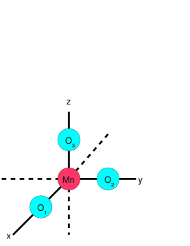
Figure 1: (Color online) Simplified crystal structure of the model. The crystal structure is assummed cubic with the unit cell containing only one Mn and three O atoms. The O atoms are labeled 1,2, and 3 to distinguish the $p-$orbitals belonging to different O atoms used to construct our Hamiltonian.

We choose 10 basis orbitals to construct our Hilbert space, which we order as the following: $|{\rm Mn}~{}e_{g~{}upper,\uparrow}\rangle$, $|{\rm Mn}~{}e_{g~{}lower,\uparrow}\rangle$, $|{\rm O}_{1}~{}p_{\uparrow}\rangle$, $|{\rm O}_{2}~{}p_{\uparrow}\rangle$, $|{\rm O}_{3}~{}p_{\uparrow}\rangle$, $|{\rm Mn}~{}e_{g~{}upper,\downarrow}\rangle$, $|{\rm Mn}~{}e_{g~{}lower,\downarrow}\rangle$, $|{\rm O}_{1}~{}p_{\downarrow}\rangle$, $|{\rm O}_{2}~{}p_{\downarrow}\rangle$, and $|{\rm O}_{3}~{}p_{\downarrow}\rangle$. Note that the distinction between $|~{}e_{g~{}upper}\rangle$ and $|~{}e_{g~{}lower}\rangle$ states is associated with the Jahn-Teller splitting. Using this set of bases we propose a Hamiltonian:

$$H = \frac{1}{N}\sum_{\bf k}\eta^{\dagger}_{\bf k}[H_{0}({\bf k})]\eta_{\bf k}+\sum_{i,\sigma,\sigma^{\prime}}Un_{u_{i}\sigma}n_{l_{i}\sigma^{\prime}}$$ (1)

$$+\sum_{i\sigma}U_{u}n_{u_{i}\uparrow}n_{u_{i}\downarrow}+\sum_{i\sigma}U_{l}n_{l_{i}\uparrow}n_{l_{i}\downarrow}$$

$$-\sum_{i}J_{H}{\bf S}_{i}{\bf.s}_{i}.$$

The first term in the Hamiltonian is the kinetic part, whereof $\eta^{\dagger}_{\bf k}$ is a row vector whose elements are the creation operators associated with the 10 basis orbitals, and $\eta_{\bf k}$ is its hermitian conjugate containing the corresponding destruction operators. Here we consider that each Mn site contributes 4 $e_{g}$ orbitals (upper and lower each of which is with up and down spins), and the three O sites contribute 6 orbitals (3 from each site each of which is with up and down spins). $[H_{0}({\bf k})]$ is a 10$\times$10 matrix in momentum space whose structure is arranged in four 5$\times$5 blocks corresponding to their spin directions as

$$[H_{0}({\bf k})]=\left[\begin{matrix}H_{0}({\bf k})_{\uparrow}&{\bf O}\\ {\bf O}&H_{0}({\bf k})_{\downarrow}\end{matrix}\right],$$ (2)

where ${\bf O}$ is a zero matrix of size 5$\times$5, and (referring to the choice of coordinates in Fig. 1)

$$H_{0}({\bf k})_{\uparrow(\downarrow)}=\left[\begin{smallmatrix}E_{JT}&0&t_{Mn-O}^{(1)}(1+e^{-ik_{x}})&t_{Mn-O}^{(1)}(1+e^{-ik_{y}})&t_{Mn-O}^{(1)}(1+e^{-ik_{z}})\\ 0&-E_{JT}&t_{Mn-O}^{(2)}(1+e^{-ik_{x}})&t_{Mn-O}^{(2)}(1+e^{-ik_{y}})&t_{Mn-O}^{(2)}(1+e^{-ik_{z}})\\ t_{Mn-O}^{(1)}(1+e^{ik_{x}})&t_{Mn-O}^{(2)}(1+e^{ik_{x}})&E_{p}&t_{O-O}(1+2e^{ik_{x}}+2e^{-ik_{y}})&t_{O-O}(1+2e^{ik_{x}}+2e^{-ik_{z}})\\ t_{Mn-O}^{(1)}(1+e^{ik_{y}})&t_{Mn-O}^{(2)}(1+e^{ik_{y}})&t_{O-O}(1+2e^{-ik_{x}}+2e^{ik_{y}})&E_{p}&t_{O-O}(1+2e^{ik_{y}}+2e^{-ik_{z}})\\ t_{Mn-O}^{(1)}(1+e^{ik_{z}})&t_{Mn-O}^{(2)}(1+e^{ik_{z}})&t_{O-O}(1+2e^{-ik_{x}}+2e^{ik_{z}})&t_{O-O}(1+2e^{-ik_{x}}+2e^{ik_{z}})&E_{p}\end{smallmatrix}\right].$$ (3)

The diagonal elements of $H_{0}({\bf k})_{\uparrow(\downarrow)}$ represent the local energies, while the off-diagonal elements represent the hybridizations between orbitals. The first two diagonal elements, i.e. $E_{JT}$ and $-E_{JT}$, correspond to the Mn${}_{e_{g}}$ orbital energies which are split due to the presumedly static Jahn-Teller distortion. Each of the remaining three diagonal elements, i.e. $E_{p}$, corresponds to the local energy of the O_2p orbital. The parameter $t_{Mn-O}^{(1)}$ ($t_{Mn-O}^{(2)}$) corresponds to hopping between the upper (lower) Mn${}_{e_{g}}$ orbital and the nearest O_2p orbital. Whereas $t_{O-O}$ corresponds to hopping between nearest O_2p orbitals.

The second term in Eq. (1) represents the Coulomb repulsions between the upper and lower Mn${}_{e_{g}}$ orbitals in a site. The third and forth terms represent the intra-orbital Coulomb repulsions. In this work, we take $U_{u}$ and $U_{l}$ to be infinity, forbidding double occupancy in each of the lower and upper Mn${}_{e_{g}}$ orbitals. Finally, the fifth term represents the double-exchange magnetic interactions between the local spins of Mn, ${\bf S}$, formed by the strong Hund’s coupling among three $t_{2g}$ electrons giving S=3/2, and the itinerant spins of the upper and lower Mn${}_{e_{g}}$ electrons, ${\bf s}$. Note that we use a well-accepted general assumption that the on-site Coulomb repulsion in each $t_{2g}$ orbital and the Hund’s coupling among the $t_{2g}$ orbitals are so strong to keep the occupancy of the three $t_{2g}$ levels fixed at high spin configuration. Thus the charge degrees of freedom of the three $t_{2g}$ electrons become frozen, and the remaining degree of freedom to be considered is the orientation of the collective spin 3/2.

Method. To solve our model, we use the Dynamical Mean Field Theory Georges-RMP1996 . First, we define the Green function of the system, which is a $10\times 10$ matrix,

$$[G({\bf k},z)] = \biggr{[}[H_{0}({\bf k})]+[\Sigma(z)]\biggr{]}^{-1},$$ (4)

with $z$ the frequency variable. Then, we coarse-grain it over the Brillouin zone as

$$[G(z)] = \frac{1}{N}\sum_{\bf k}[G({\bf k},z)].$$ (5)

In defining $[G({\bf k},z)]$, all the interaction parts of the Hamiltonian (all terms other than the kinetic part), are absorbed into a momentum-independent self energy matrix, $[\Sigma(z)]$, which will be solved self-consistently. Note that in this algorithm, we need to go over the self-consistent loops in both Matsubara ($z=i\omega_{n}+\mu$) and real frequency ($z=\omega+i0^{+}$).

On taking $U_{u}$ and $U_{l}$ to be infinity, to some approximation, we forbid the double occupancies in states $|{\rm Mn}~{}e_{g~{}upper,\uparrow}\rangle$, $|{\rm Mn}~{}e_{g~{}lower,\uparrow}\rangle$, $|{\rm Mn}~{}e_{g~{}upper,\downarrow}\rangle$, and $|{\rm Mn}~{}e_{g~{}lower,\downarrow}\rangle$ by throwing them out of our Hilbert space. To do this, according to the structure of Hamiltonian matrix in Eqs. (2) and (3), we multiply the weights of all the diagonal elements with indices 1, 2, 6, and 7, and all the corresponding off-diagonal elements connecting any pair of them by a half. Thus, after obtaining the matrix $[G(z)]$ from Eq. (5), the effective $[G(z)]$ (let’s call it $[G(z)]_{\rm eff}$) can be obtained by multiplying each of the following blocks of $[G(z)]$ by a half, while keeping the remaining elements unchanged, that is

$$\left[\begin{matrix}G_{11}&G_{12}\\ G_{21}&G_{22}\\ \end{matrix}\right] \Rightarrow \frac{1}{2}\left[\begin{matrix}G_{11}&G_{12}\\ G_{21}&G_{22}\\ \end{matrix}\right],$$

$$\left[\begin{matrix}G_{16}&G_{17}\\ G_{26}&G_{27}\\ \end{matrix}\right] \Rightarrow \frac{1}{2}\left[\begin{matrix}G_{16}&G_{17}\\ G_{26}&G_{27}\\ \end{matrix}\right],$$

$$\left[\begin{matrix}G_{61}&G_{62}\\ G_{71}&G_{72}\\ \end{matrix}\right] \Rightarrow \frac{1}{2}\left[\begin{matrix}G_{61}&G_{62}\\ G_{71}&G_{72}\\ \end{matrix}\right],$$

$$\left[\begin{matrix}G_{66}&G_{67}\\ G_{76}&G_{77}\\ \end{matrix}\right] \Rightarrow \frac{1}{2}\left[\begin{matrix}G_{66}&G_{67}\\ G_{76}&G_{77}\\ \end{matrix}\right].$$ (6)

The “mean-field” Green function can then be extracted as

$$[{\cal G}(z)]=\biggr{[}[G(z)]_{\rm eff}^{-1}+[\Sigma(z)]\biggr{]}^{-1}.$$ (7)

Next, we construct the local self energy matrix, $[\Sigma_{n_{l}}(z)]$, corresponding to the second and the fifth terms of the Hamiltonian. Here $n_{l}\in\{0,1\}$ is the occupation number of the lower Mn${}_{e_{g}}$ orbital. The elements of the $10\times 10$ matrix $[\Sigma_{n_{l}}(z)]$ are all zero except for the blocks

$$\left[\begin{matrix}\Sigma_{11}&\Sigma_{16}\\ \Sigma_{61}&\Sigma_{66}\\ \end{matrix}\right] = \left[\begin{smallmatrix}-J_{H}S\cos\theta+n_{l}U&-J_{H}S(\cos\phi+i\sin\phi)\\ -J_{H}S(\cos\phi-i\sin\phi)&J_{H}S\cos\theta+n_{l}U\end{smallmatrix}\right],$$

$$\left[\begin{matrix}\Sigma_{22}&\Sigma_{27}\\ \Sigma_{72}&\Sigma_{77}\\ \end{matrix}\right] = \left[\begin{smallmatrix}-J_{H}S\cos\theta&-J_{H}S(\cos\phi+i\sin\phi)\\ -J_{H}S(\cos\phi-i\sin\phi)&J_{H}S\cos\theta\end{smallmatrix}\right].$$

The local interacting Green function matrix is then calculated through

$$[G_{n_{l}}(z)]=\biggr{[}[{\cal G}(z)]^{-1}-[\Sigma_{n_{l}}(z)]\biggr{]}^{-1},$$ (9)

where $\theta$ and $\phi$ are the corresponding angles representing the direction of ${\bf S}$ in the spherical coordinate.

For each Mn site with a given $n_{l}$, the probability of Mn spin ${\bf S}$ having a direction with angle $\theta$ with respect to the direction of magnetization (which is defined as the $z-$axis) is given by

$$P_{n_{l}}(\cos\theta)=\frac{e^{-S_{n_{l}}(\cos\theta)}}{Z_{n_{l}}},$$ (10)

where

$$Z_{n_{l}}=\int d(\cos\theta)e^{-S_{n_{l}}(\cos\theta)}$$ (11)

is the local partition function, and

$$S_{n_{l}}(\cos\theta)=-\sum_{n}\ln\det[G_{n_{l}}(i\omega_{n})]e^{-i\omega_{n}0^{+}}$$ (12)

is the effective action.

We need to average $[G_{n_{l}}(z)]$ over all possible $\theta$ and $n_{l}$ values as

$$[G(z)]_{\rm ave} = (1-\langle n_{l}\rangle)\int d(\cos\theta)P_{0}(\cos\theta)[G_{0}(z)]$$ (13)

$$+~{}\langle n_{l}\rangle\int d(\cos\theta)P_{1}(\cos\theta)[G_{1}(z)],$$

where $\langle n_{l}\rangle$ is the average occupation of lower Mn${}_{e_{g}}$ orbital. The new self energy matrix is extracted through

$$[\Sigma(z)]=[{\cal G}(z)]^{-1}-[G(z)]_{\rm ave}^{-1}~{}.$$ (14)

Finally, we feed this new self energy matrix back into the definition of Green function in Eq. (4), and the iteration process continues until $[\Sigma(z)]$ converges.

After the self-consistency is achieved, we can compute the density of states as

$${\rm DOS}(\omega)=-\frac{1}{\pi}{\rm ImTr}[G(\omega+i0^{+})]~{}.$$ (15)

We can also compute the optical conductivity tensor as

$$\sigma_{\alpha\beta}(\omega)=\frac{\pi e^{2}}{\hbar ad}\int d\nu\biggr{(}\frac{f(\nu,T)-f(\nu+\omega,T)}{\omega}\biggr{)}\times~{}~{}~{}~{}~{}~{}~{}~{}$$

$$\frac{1}{N}\sum_{\bf k}~{}{\rm Tr}[v_{\alpha}({\bf k})][A({\bf k},\nu)][v_{\beta}({\bf k})][A({\bf k},\nu+\omega)],$$

where $[v_{\lambda}({\bf k})]=\partial[H_{0}({\bf k})]/\partial k_{\lambda}$ is the Cartesian component of the velocity matrix, $[A({\bf k},\nu)]=\big{(}[G({\bf k},\omega+i0^{+})]-[G({\bf k},\omega-i0^{+})]\big{)}/(2\pi i)$ the spectral function matrix, and $f(\nu,T)$ the Fermi distribution function. Note that the dimensional pre-factor $\pi e^{2}/(\hbar ad)$ Georges-RMP1996 with $d=3$ is introduced to restore the proper physical unit, since the rest of the expression was derived by setting $e=\hbar=a=1$. In our model, the system is isotropic, and we are only interested in the tranverse components $\sigma_{\alpha\alpha}(\omega)\equiv\sigma(\omega)$, which are equal for all $\alpha\in\{x,y,z\}$.

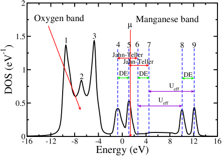
Figure 2: (Color online) Calculated density of states (DOS). See text for the parameter values used in this figure and the detailed explanation of the structures of the DOS.

Results. Our calculated density of states is shown in Fig. 2. The parameter values used for this calculation are $E_{JT}$=0.5eV, $E_{p}$=-6.5eV, $t_{Mn-O}^{(1)}$=1.2eV, $t_{Mn-O}^{(2)}$=0.8eV, $t_{O-O}$=0.6eV, $U$=10eV, $J_{H}$=1.5eV, $a$=3.9345Å, and $T\approx 194$K (corresponding to $\beta\equiv 1/T=60$ eV^-1). These parameter values are chosen considering rough estimates given in other papers Millis-PRB1996 ; Ramakrishnan-PRL2004 ; Picket-PRB1996 and adjusted so as to give best agreement with the experimental optical conductivity data in Ref. Rusydi-PRB2008 . The DOS is normalized such that the integrated area is equal to 8, since in each unit cell there are 6 orbitals coming from oxygens and effectively 2 from manganeses, considering the restriction given by relation (Theory of high energy optical conductivity and the role of oxygens in manganites). The chemical potential is self-consistently adjusted to satisfy the electron filling of 6+(1-$x$)=6.7, mimicking the situation of La_1-xCa_xMnO₃ for $x=0.3$. The structures of the density of states can be explained as the following. The three peaks labeled 1,2,3 result from the fact that there are three oxygen atoms in a unit cell, where the degeneracy is broken into three levels by the hybridization between $2p$ orbitals of the neighboring oxygen atoms. The structures labeled with 4 through 9 result from the $e_{g}$ orbitals of mangeneses. As shown in the figure, there are three mechanisms that split the Mn${}_{e_{g}}$ states into 6 levels: static Jahn-Teller (JT) distortion, Coulomb repulsion U_eff) between lower and upper JT-split $e_{g}$ states, the double-exchange (DE) interaction between spins of electrons in the lower and upper JT-split states and the Mn spins formed by the Hund’s coupling among the Mn $t_{2g}$ electrons Note1 .

Figure 3 shows our calculated optical conductivity for $T\approx 194$K ($>T_{FM}$). The ferromagnetic transition temperature for this set of parameters is roughly $T_{FM}\approx 160$K (based on extrapolation of the mean-field trend). The parameter values for $T\approx 194$K are the same as those used in Fig. 2. In Figure 3, we demonstrate how we tune the the profile of the optical conductivity to achieve the best resemblance with the experimental data in Ref. Rusydi-PRB2008 . It is important to note that our model is not meant to address the dc conductivity, as we already anticipate that it cannot form an insulating (or nearly insulating) phase at $T>T_{FM}$, possibly due to not incorporating electron-phonon interactions Millis-PRB1996 ; Ramakrishnan-PRL2004 ; Ederer-PRB2007 . Rather, our goal is to show how this simple model can capture qualitatively the general profile of the optical conductivity from about 1 eV away from the Drude peak up to 22 eV (the energy limit of the experimental data).

On calculating the optical conductivity from Eq. (Theory of high energy optical conductivity and the role of oxygens in manganites) we introduce an imaginary self energy for the O_2p states, $-i\Gamma$, where $\tau=1/\Gamma$ corresponds to the lifetime of the O_2p states. The red curve in Fig. 3 shows the result if we use the self-consistent chemical potential, $\mu$, in Eq. (Theory of high energy optical conductivity and the role of oxygens in manganites). Here, we observe that the resulting profile around the medium energy region ($\approx$ 5-11 eV) does not satisfactorily resembles that of the experimental data in Ref. Rusydi-PRB2008 , since some spectral weight seems to be missing in that region. We argue that the reason for this is related to the fact that our self-consistent chemical potential, $\mu$, does not lie inside a pseudogap as it probably would if we incorporate electron-phonon interactions. In this model, we only have a pseudogap that results from the double-exchange splitting, where $\mu$ falls slightly to the right outside of this pseudogap. To remedy the missing of spectral weight, we slightly shift the position of chemical potential to the left, i.e. from $\mu$ to $\mu^{*}$ as shown in the inset of Fig. 3. Using this new chemical potential, $\mu^{*}$, the resulting optical conductivity, shown in the blue curve, resembles the experimental data better. This suggests that the true chemical potential may actually lie inside a pseudogap similar to the situation as though it lies at $\mu^{*}$. (Note that, as long as considering the optical conductivity region about 1 eV away from the Drude peak, choosing $\mu^{*}$ between 0.1 and 0.9 eV, i.e. around the valley, lead to similar results.) Although the profile of the blue curve is already better than the red one, it still has more pronounced stuctures than the actual experimental data does. To further tune the calculated optical conductivity to better resemble the experimental data, we find that the overly pronounced structures can be broadened by enlarging the O_2p imaginary self energy upto $\Gamma=0.6$ eV. The result after the broadening, which is shown in the black curve, looks very similar to the experimental results shown in Fig. 2(b) of Ref. Rusydi-PRB2008 (replotted in the inset of Fig. 4). This similarity in both magnitude and profile of the energy dependence may be a good measure of the validity of our model.

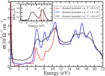
Figure 3: (Color online) Calculated optical conductivity. Main panel: The red and blue curves represent the calculated optical conductivites for different position of chemical potential, $\mu$ and $\mu^{*}$, respectively, using only a small broadening ($\Gamma$=0.1 eV). The black curve represents the result using chemical potential at $\mu^{*}$ with a bigger broadening ($\Gamma$=0.6eV). Inset: Region in the density of states showing how the position of chemical potential is shifted. See text for detailed explanation.

Now we discuss how the model captures the spectral weight transfer when temperature is decreased from $T>T_{FM}$ to $T<T_{FM}$. First, we divide the energy range into three regions: I (low:$\approx$1-3eV), II (medium:$\approx$3-12eV), and III (high:$\gtrsim$12eV), following the division made for the experimental data in Ref. Rusydi-PRB2008 , except that we exclude the region around the Drude peak from our discussion, since to obtain the correct values of conductivity in that region requires a more accurate description of the renormalized band structure around the chemical potential. If we decrease temperature from the paramagnetic to ferromagnetic phase while keeping all the parameters constant, we find no significicant change in the optical conductivity, thus spectral weight transfer does not occur in this way. If we inspect how Eq. (Theory of high energy optical conductivity and the role of oxygens in manganites) determines the optical conductivity, we see that the change in optical conductivity may become more significant if either the spectral function, $[A({\bf k},\nu)]$, or the velocity operator, $[v_{\alpha}({\bf k})]$, changes significantly while temperature changes. Within our model this can only be accomodated if we allow some parameters to depend on temperature by some manner. By comparing the structures of optical conductivity and the corresponding DOS profile, it is clear that the spectral weight in the medium energy region comes mostly from transitions from $O_{2p}$ to lower Mn${}_{e_{g}}$ states, while in the high energy region from $O_{2p}$ to upper Mn${}_{e_{g}}$ states. This fact may suggest that the hopping parameters $t_{Mn-O}^{(1)}$ and $t_{Mn-O}^{(2)}$ depend on temperature. Furthermore, since the spectral weight transfer occurs most notably across and below $T_{FM}$, the temperature dependence of $t_{Mn-O}^{(1)}$ and $t_{Mn-O}^{(2)}$ may be related to spin correlation.

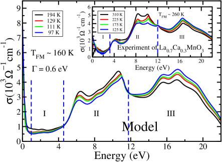
Figure 4: (Color online) Spectral weight transfer in the optical conductivity. Main panel: Results of the model. Excluding the region containing the Drude peak (0-1eV), the energy range is divided into three regions I,II, and III. The black curve represents the optical conductivity in the paramagnetic phase, while the red, green, and blue curves correspond successively to lower temperatures in the ferromagnetic phase Note2 . The borders between regions I-II and II-III, denoted by the blue vertical dashed lines, are defined such that the curves are crossing at these energies. Inset: A replot of the corresponding experimental data from Ref. Rusydi-PRB2008 for comparison.

The actual interplay resulting in such a temperature dependence is believed to be very complicated, since it may involve orbital effects on the dynamic electron-phonon coupling and spin correlation. In that regard, our present model, which is not an ab initio based model, cannot naturally capture these temperature effects. Thus, to capture the plausible physics within our present model, we turn to the phenomenological approach by parametrizing the totally non-trivial temperature effecs on hopping integrals through magnetization. In the simplest level, we may assume a linear dependence of the hopping integrals $t_{Mn-O}^{(1)}$ and $t_{Mn-O}^{(2)}$ on the magnetization. Hence, we may write

$$t_{Mn-O}^{(1)}(M)=t_{Mn-O}^{(1)}(0)\biggr{(}1+c_{1}\frac{M}{M_{s}}\biggr{)},$$ (17)

$$t_{Mn-O}^{(2)}(M)=t_{Mn-O}^{(2)}(0)\biggr{(}1+c_{2}\frac{M}{M_{s}}\biggr{)},$$ (18)

where $M/M_{s}$ is the ratio of magnetization to the saturated magnetization, and $c_{1}$, and $c_{2}$ are constants.

Using relations (17) and (18), taking $t_{Mn-O}^{(1)}(0)$=1.2 eV, $t_{Mn-O}^{(2)}(0)$=0.8 eV, $c_{1}\approx 0.23$, and $c_{2}\approx$ -0.35, at $T$=97K for which $M/M_{s}$=0.357, for instance, we obtain that $t_{Mn-O}^{(1)}$ is enhanced to be $\approx$ 1.3 eV, while $t_{Mn-O}^{(1)}$ is suppressed to be $\approx$ 0.7 eV. The results for four different temperatures are shown in Fig. 4. As shown in the main panel, our calculation shows that the spectral weight simultaneously decreases (increases) in the medium (high) energy region of the optical conductivity as the system becomes ferromagnetic Note3 . Our calculation also produces a less noticeable decrease of the spectral weight in the low energy region as observed in the experimental data (see the inset). In both the main panel and the inset, the black curve represents the optical conductivity in the paramagnetic phase, while the red, green, and blue curves correspond successively to lower temperatures in the ferromagnetic phase. If we define the positions of the borders between energy regions I-II and II-III such that all the curves are crossing at these energies, we obtain that theoretical values of these energies are similar to the experimental ones. Note that the temperatures varied in the theoretical and the experimental results should not be compared quantitatively, since the theoretical $T_{FM}$ is about 100 K too small compared to the experimental one, possibly due to neglecting other possible exchange interactions in our model. Despite this, we believe that any improvement of $T_{FM}$ by such additional terms would not change the physics presented in this paper. To show the difference in the density of states between paramagnetic and ferromagnetic phases, we display the spin dependent DOS for $T\approx 194$K and $T\approx 97$K in Fig. 5.

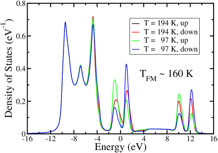
Figure 5: (Color online) Spin-dependent density of states. The black and the red curves lie on top of each other as the spin-up and spin-down components of the DOS are identical in the paramagnetic phase. While, the green and the blue curves look quite distinct as DOS becomes polarized in the ferromagnetic phase.

To demonstrate further how the spectral-weight transfers in our model compare with the experimetal results, we display the relative spectral-weight changes for different regions of energy in Fig. 6. Comparing results in Fig. 6(a) and (b), it is clear that for every region of energy, I (low), II (medium), and III (high), (excluding 0-1 eV), our calculations give exactly same trends as those shown by the experimental results. These suggest that the ingredients incorporated in our model are adequate to explain the occurrence of spectral-weight transfers in La_1-xCa_xMnO₃ in the energy range up to 22 eV. In that respect, one may argue, for instance, that the high-spin state ($S=3/2$) of the $t_{2g}$-electrons may become unstable as the system is optically excited by high-energy photons. Accordingly, transitions from high to low-spin states, or excitations of electrons from $t_{2g}$ to $e_{g}$ levels may occur. Our present model does not incorporate those possibilities. However, our calculations prove that the model is capable to obtain the spectral-weight transfers with good qualitative agreement with the experimental results, thus suggesting that such other contributions may be minor or irrelevant.

The inset of Fig. 6(a) is to show that for 0-1 eV region our result does not agree with the experiment, since it does not capture the insulator-metal transition. As mentioned earlier, we argue that this is due to our model not incorporating the dynamic Jahn-Teller phonons and their interactions with electrons, which may be responsible to form an insulating gap in the paramagnetic phase. The incorporation of such terms to improve our present model is under our on-going study.

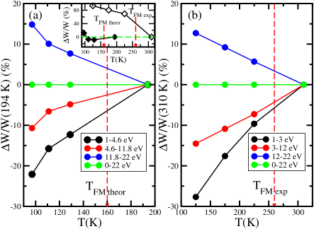
Figure 6: (Color online) Relative spectral-weight changes. $\Delta W(T)/W$ from (a) our calculations, and (b) the experimental results of Ref. Rusydi-PRB2008 , for different regions of energy. $\Delta W/W$ is defined as spectral-weight difference $\Delta W=\int_{\omega_{1}}^{\omega_{2}}\big{(}\sigma(\omega,T)-\sigma(\omega,T_{PM})\big{)}d\omega$ normalized to $W(T_{PM})=\int_{\omega_{1}}^{\omega_{2}}\sigma(\omega,T_{PM})d\omega$, where in this case $T_{PM}$ is 194 K in (a) and 310 K in (b). Positions of the theoretical and the experimental $T_{FM}$ are indicated by vertical red dashed lines in each panel. Inset in (a) is comparison between $\Delta W(T)/W$ from the calculations (black filled diamonds) and from the experiments of Ref. Rusydi-PRB2008 (black empty diamonds) for 0-1 eV region. The horizontal green dashed line in the inset is just to highlight the zero position of $\Delta W/W$.

Conclusion. In conclusion, we have developed a model to explain the structures and the spectral weight transfer occuring in the optical conductivity of La_1-xCa_xMnO₃ for $x=0.3$. The key that makes our model work in capturing the structures of the optical conductivity at medium and high energies is the inclusion of O_2p orbitals into the model.

Further, by parametrizing the hopping integrals through magnetization, our model captures the spectral weight transfer as temperature is decreased across the ferromagnetic transition temperature. Our calculation based on this phenomenological parameters suggests that the ferromagnatic ordering increases the hopping parameter connecting the O_2p orbitals and the upper Mn${}_{e_{g}}$ orbitals, while simultaneously decreasing the hopping parameter connecting O_2p orbitals and the lower Mn${}_{e_{g}}$ orbitals. Although we have yet to check whether or not this scenario works in a more complete model incorporating the dynamic electron-phonon coupling, we conjecture that this may be of important part that contributes to the mechanism of insulator to metal transition in manganites.

Overall, our results demonstrate the strength of our model that one may have to consider as the minimum model before adding other ingredients in order to properly explain the insulator-metal transition or other features in correlated electron systems such as manganites.

Acknowledgement. MAM and AR thank George Sawatzky and Seiji Yunoki for their valuable comments and suggestions. This work is supported by NRF-CRP grant ”Tailoring Oxide Electronics by Atomic Control” NRF2008NRF-CRP002-024, NUS YIA, NUS cross faculty grant and FRC. We acknowledge the CSE-NUS computing centre for providing facilities for our numerical calculations. Work at NTU was supported in part by a MOE AcRF Tier-1 grant (grant no. M52070060).

References

- (1)
- (2) S. Jin, T. H. Tiefel, M. McCormack, R. A. Fastnacht, R. Ramesh, and L. H. Chen, Science 264, 413 (1994).
- (3) For a general review on the structure and transport in manganites, see M. B. Salamon and M. Jaime, Rev. Mod. Phys. 73, 583 (2001) and references therein.
- (4) S.-W. Cheong and M. Mostovoy, Nat. Mater. 6, 13 (2007).
- (5) E. Saitoh, S. Okamoto, K. T. Takahashi, K. Tobe, K. Yamamoto, T. Kimura, S. Ishihara, S. Maekawa and Y. Tokura, Nature (London) 410, 180 (2001).
- (6) A. Moreo, S. Yunoki, and E. Dagotto, Science 283, 2034 (1999).
- (7) A. Nucara, A. Perucchi, P. Calvani, T. Avelage, and D. Emin, Phys. Rev. B 68 174432 (2003).
- (8) P. W. Anderson and H. Hasegawa, Phys. Rev. 100, 675 (1955).
- (9) P. -G. de Gennes, Phys. Rev. 118, 141 (1960).
- (10) M. Quijada, J. ČČerne, J. R. Simpson, H. D. Drew, K. H. Ahn, A. J. Millis, R. Shreekala, R. Ramesh, M. Rajeswari, and T. Venkatesan, Phys. Rev. B 58, 16093 (1998).
- (11) V. A. Amelitchev, B. Güüttler, O. Yu. Gorbenko, A. R. Kaul, A. A. Bosak, and A. Yu. Ganin, Phys. Rev. B 63, 104430 (2001).
- (12) Pengcheng Dai, J. A. Fernandez-Baca, E. W. Plummer, Y. Tomioka, and Y. Tokura, Phys. Rev. B 64, 224429 (2001).
- (13) A. J. Millis, R. Mueller, and Boris I. Shraiman, Phys. Rev. B 54, 5389 (1996) and Phys. Rev. B 54, 5405 (1996).
- (14) T. V. Ramakrishnan, H. R. Krishnamurthy, S. R. Hassan, and G. Venketeswara Pai, Phys. Rev. Lett. 92, 157203 (2004)
- (15) A. J. Millis, Boris I. Shraiman, and R. Mueller, Phys. Rev. Lett. 77, 175 (1996).
- (16) O. Céépas, H. R. Krishnamurthy, and T. V. Ramakrishnan, Phys. Rev. Lett. 94, 247207 (2005)
- (17) Yu-Li Lee and Yu-Wen Lee, Phys. Rev. B 75, 064411 (2007).
- (18) M. Stier and W. Nolting, Phys. Rev. B 75, 144409 (2007).
- (19) Rong Yu, Shuai Dong, Cengiz ŞŞen, Gonzalo Alvarez, and Elbio Dagotto, Phys. Rev. B 77, 214434 (2008).
- (20) Chungwei Lin and Andrew J. Millis, Phys. Rev. B 78, 174419 (2008).
- (21) J. Zaanen, G. A. Sawatzky, and J. W. Allen, Phys. Rev. Lett. 55, 418 (1985).
- (22) M. B. J. Meinders, H. Eskes, and G. A. Sawatzky, Phys. Rev. B 48, 3916 (1993).
- (23) W. G. Yin, D. Volja, and W. Ku, Phys. Rev. Lett. 96, 116405 (2006).
- (24) Philip Phillips, Rev. Mod. Phys. 82, 1719 (2010).
- (25) A. Rusydi, R. Rauer, G. Neuber, M. Bastjan, I. Mahns, S. Müüller, P. Saichu, B. Schulz, S. G. Singer, A. I. Lichtenstein, D. Qi, X. Gao, X. Yu, A. T. S. Wee, G. Stryganyuk, K. Dörr, G. A. Sawatzky, S. L. Cooper, and M. Rübhausen, Phys. Rev. B 78, 125110 (2008).
- (26) W.E. Picket and J.D. Singh, Phys. Rev. B 53, 1146 (1996).
- (27) Antoine Georges, Gabriel Kotliar, Werner Krauth, and Marcelo J. Rozenberg, Rev. Mod. Phys. 68, 13 (1996).
- (28) Claude Ederer, Chungwei Lin, and Andrew J. Millis, Phys. Rev. B 76, 155105 (2007).
- (29) If the double-exchange (DE) interactions were not there, each of the pairs of 4-5, 6-7, and 8-9 would merge into one. The 4-5 pair corresponds to the lower part of the JT-split states, while the 6-7 and 8-9 pairs correspond to the upper part. The 6-7 and 8-9 pairs are further split by the Coulomb repulsion (U) between lower and upper JT-split states. Namely, when the lower JT-split level (4-5) is unoccupied, the upper level is given by 6-7. Whereas, if 4-5 is occupied, the corresponding upper level is given by 8-9.
- (30) If one shifts but to remain around the valley, or changes the value of from 1 to 6 eV, the effect of weight transfer is still captured with the crossover between regions of medium and high energy being relatively unchanged (within 1 eV), while the amount of weight transferred may change by not more than one hundred percent.
- (31) Since the self-consistently computed chemical potentials () we found for the PM and FM phases are almost the same, we choose to define in PM and FM phases by shifting their corresponding to the left by the same amount. This way, for PM and FM phases are pretty much the same.