Non-linear phenomena in time-dependent density-functional theory: What Rabi physics can teach us

Abstract

Through the exact solution of a two-electron singlet system interacting with a monochromatic laser we prove that all adiabatic density functionals within time-dependent density-functional theory are not able to discern between resonant and non-resonant (detuned) Rabi oscillations. This is rationalized in terms of a fictitious dynamical exchange-correlation (xc) detuning of the resonance while the laser is acting. The non-linear dynamics of the Kohn-Sham system shows the characteristic features of detuned Rabi oscillations even if the exact resonant frequency is used. We identify the source of this error in a contribution from the xc-functional to the set of non-linear equations that describes the electron dynamics in an effective two-level system. The constraint of preventing the detuning introduces a new strong condition to be satisfied by approximate xc-functionals.

I Introduction

Despite of the success of linear-response schemes to describe excitations of many electron systems, many physical processes stemming from the interaction of light with matter are non-linear in nature (i.e. photo-reactivity, population quantum control, etc). A prototype effect, ubiquitous in many fields of physics, are Rabi oscillations between the ground and an excited state when a monochromatic laser with a frequency close to the resonance is applied. The dipole moment of the system then shows fast oscillations with the frequency of the applied laser and an envelope that oscillates with the frequency attributed to the transition from the ground to the excited state (Rabi frequency). It is one of the few analytically solvable cases of non-linear electron dynamics where the population of states changes dramatically in time. Thus, Rabi dynamics provides a firm ground to derive fundamental properties of the exact exchange-correlation (xc) functional of time-dependent density-functional theory (TDDFT) RG1984 ; TDDFT2006 . This is one of the scopes of the present paper together with providing a sound description of laser induced population processes within TDDFT. We remark that it was recently concluded that Rabi oscillations cannot be described within a finite-level model in TDDFT BauerRugg . The authors observed that the dipole moment in an adiabatic exact exchange (EXX) calculation shows the characteristic Rabi oscillations while the density does not show a transition to the excited state.

Here, we show that for all adiabatic functionals the observed oscillations in the dipole moment can indeed be described as Rabi oscillations, however, with a non-resonant laser frequency. The employed adiabatic approximation results in a detuning, i.e. the system is driven out of resonance by the change in the Kohn-Sham (KS) potential which is due to the change in the density. The failure of adiabatic density functionals to correctly describe Rabi oscillations has some resemblance to well-known problems of describing double and charge transfer excitations MZCB2004 ; DH2004 and ionization processes PG1999 that were all traced back to the lack of memory in the functional. In the present work we use the example of Rabi oscillations to identify the physics behind the failure of adiabatic constructions to describe resonant non-linear dynamics. Our results show that the problems are not limited to adiabatic TDDFT but affect any mean-field theory.

The paper is organized as follows. In Section II we derive the analytic solution for Rabi oscillations in a many-body interacting system and apply this solution to compute the dipole moment and the populations of an exactly solvable one-dimensional model. In Section III we map the interacting problem onto a non-interacting Kohn-Sham one and carry out numerical time propagations using two different adiabatic approximations, ALDA and EXX. We also derive analytic expressions for the dipole moment and the populations in the KS system within the adiabatic EXX approximation and discuss and quantify the appearing dynamical detuning. We conclude our paper with a summary and outlook in Section IV.

II Rabi dynamics in interacting many-body systems

The Hamiltonian for an interacting non-relativistic $N$-electron system coupled to a laser field of the form ${\cal E}(t)={\cal E}_{0}\sin(\omega t)$ in dipole approximation is given by

$$\hat{H}=\hat{T}+\hat{V}_{ext}+\hat{V}_{ee}+\sum_{j=1}^{N}{\bf r}_{j}{\bf{\cal E}}(t)$$ (1)

with $\hat{T}$ being the kinetic energy, $\hat{V}_{ext}$ describing the external potential, and $\hat{V}_{ee}$ being the electron-electron interaction (atomic units $m=e=\hbar=1$ are used throughout the paper). We denote the eigenstates and eigenvalues of Hamiltonian (1) with $\psi_{k}$ and $\epsilon_{k}$, respectively. In order for Rabi’s solution to be valid (for a detailed discussion see e.g. Ref. QMTD, ), the system under study needs to be an effective two-level system reducing the solution space to $\psi_{g}$ (ground state) and $\psi_{e}$ (dipole allowed excited state) with eigenenergies $\epsilon_{g}$ and $\epsilon_{e}$. The system then has a resonance at $\Delta=\epsilon_{e}-\epsilon_{g}$. For a generic situation the two-level approximation should be valid if the laser frequency $\omega$ is close to the resonance, and the amplitude of the driving field is not too strong to disturb the rest of the spectrum. These conditions can be formalized as follows

$${\delta}<<{\Delta},\quad\Omega_{0}<<\omega,$$ (2)

where $\delta=\omega-\Delta$ is the detuning from the two-level resonance and $\Omega_{0}=d_{eg}{\cal E}_{0}$ is the resonant Rabi frequency, with $d_{eg}=\langle\psi_{g}|\sum_{j}\hat{{\bf r}}_{j}|\psi_{e}\rangle$ being the dipole transition matrix element.

For an effective two-level system the time-dependent many-body state $|\Psi(t)\rangle$ can be written as a linear combination of both ground and excited states, i.e.

$$|\psi(t)\rangle=a_{g}(t)|\psi_{g}\rangle+a_{e}(t)|\psi_{e}\rangle$$ (3)

with $|a_{g}(t)|^{2}=n_{g}(t)$ and $|a_{e}(t)|^{2}=n_{e}(t)$ being the time-dependent populations of the ground and excited states, respectively. Normalization of the wave functions implies $n_{g}(t)+n_{e}(t)=1$. Using Eq. (3) to compute the dipole moment $d(t)=\langle\psi(t)|\sum_{j}\hat{{\bf r}}_{j}|\psi(t)\rangle=d_{eg}2Re[a_{g}^{*}(t)a_{e}(t)]$ we obtain

$$d(t)=2d_{eg}\sqrt{n_{g}(t)n_{e}(t)}\cos(\omega t+\varphi(t)),$$ (4)

where $\varphi(t)$ is a slowly varying (on the scale of $1/\omega$) part of the phase difference of the coefficients $a_{g}(t)$ and $a_{e}(t)$. The Rabi dynamics is encoded in the envelope of the dipole moment through the time dependence of $n_{g}(t)$ and $n_{e}(t)$. After the two-level projection the time-dependent Schrödinger equation $i\partial_{t}|\psi(t)\rangle=\hat{H}|\psi(t)\rangle$ reduces to the form

$$i\partial_{t}\left({\begin{array}[]{c}a_{g}(t)\\ a_{e}(t)\\ \end{array}}\right)=\left({\begin{array}[]{cc}\epsilon_{g}&d_{eg}{\cal E}(t)\\ d_{eg}{\cal E}(t)&\epsilon_{e}\\ \end{array}}\right)\left({\begin{array}[]{c}a_{g}(t)\\ a_{e}(t)\end{array}}\right).$$ (5)

The conditions (2) imply the existence of two well-separated timescales: one governed by the external frequency $\omega$ and the other determined by the Rabi frequency $\Omega_{0}$, the frequency of the oscillations between the ground and the excited state. This timescale separation allows for the use of the rotating wave approximation (RWA) QMTD leading to the following differential equation for $n_{e}(t)$ (for an outline of the derivation see Appendix A)

$$\partial^{2}_{t}n_{e}(t)=-\left(\delta^{2}+\Omega_{0}^{2}\right)n_{e}(t)+\frac{1}{2}\Omega_{0}^{2}$$ (6)

with initial conditions $n_{e}(0)=0$ and $\partial_{t}{n}_{e}(0)=0$. Eq. (6) describes a harmonic oscillator with a restoring force which increases with increasing detuning $\delta$ (see potentials for different detunigs $\delta$ in Fig. 3). Thus, increasing $\delta$ results in a squeezing of the harmonic potential leading to a decrease of the amplitude of the oscillations according to $n_{e}^{\mathrm{max}}=\Omega_{0}^{2}/(\Omega_{0}^{2}+\delta^{2})$ and a larger Rabi frequency (see Fig. 1).

In order to investigate the description of Rabi oscillations within TDDFT we analyze a one-dimensional (1D) two-electron model system which has the advantage that it can be solved exactly HFCVMTR2011 . For ease of comparison we choose the same model as in BauerRugg with the external potential

$$V_{ext}=-2/\sqrt{x^{2}+1}$$ (7)

and the electron-electron interaction being of soft-Coulomb type, i.e. $V_{ee}=1/\sqrt{(x_{1}-x_{2})^{2}+1}$. The eigenfunctions and eigenvalues are obtained by diagonalization of the Hamiltonian (1) using the octopus code octopus ; octopus2 . The calculations are performed in a box from $-100$ to $100$ bohr with a spacing of $0.2$ bohr. The obtained eigenvalues are $\epsilon_{g}=-2.238$ Ha and $\epsilon_{e}=-1.705$ Ha, and the static dipole matrix element is $d_{eg}=1.104$. In order to induce Rabi oscillations, a laser field of the form ${\cal E}(t)={\cal E}_{0}\sin(\omega t)$ is turned on at $t=0$, with ${\cal E}_{0}=0.0125\omega$ which ensures conditions (2) are satisfied. The frequency $\omega$ of the applied field has been chosen to be close to the resonance $\Delta=\epsilon_{e}-\epsilon_{g}$.

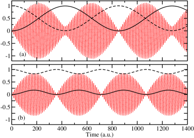
Figure 1: Dipole moment (red) and populations $n_{e}$ (solid black line) and $n_{g}$ (dashed black line) from the analytic solution of (5) using ${\cal E}_{0}=0.0125\omega$ for detuning $\delta=0.08\Omega_{0}$ ($0.0006$ Ha) (a) and $\delta=2.2\Omega_{0}$ ($0.016$ Ha) (b).

In Fig. 1 the time-dependent dipole moment $d(t)$ and the populations $n_{g}(t)$ and $n_{e}(t)$ for $\delta=0.08\Omega_{0}$ and $\delta=2.2\Omega_{0}$ are shown. The effect of the detuning manifests in an incomplete population of the excited state and a consequent decrease in the amplitude of the envelope of $d(t)$ that is proportional to $\sqrt{n_{g}n_{e}}$. For small detuning the minima and the maxima of $n_{e}$ coincide with minima of the envelope, but for larger detuning the dipole moment only goes to zero for the minima of $n_{e}$. In Fig. 1a, $\delta$ is very small but non-zero leading to the appearance of a neck at the odd minima of the envelope function which coincide with the minima of $n_{g}$. The neck increases with increasing $\delta$ and evolves into a maximum for Fig. 1b. Thus, the first minimum of Fig. 1b corresponds to one complete cycle and can be identified with the second minimum in 1a. We note that looking only at the dipole moment is insufficient to discern between resonant and detuned Rabi oscillations, only studying the population $n_{e}$ of the excited state provides access to the complete picture. A comparison between the analytic solution of Eqs. (4)-(6) and the results of the time-propagation with the octopus code shows perfect agreement, which confirms that the conditions (2) are fulfilled for the chosen values of ${\cal E}_{0}$ and $\omega$.

III Rabi oscillations in the Kohn Sham system

In TDDFT the interacting system is mapped onto a non-interacting KS system which reproduced the correct density $\rho(r,t)$ RG1984 ; TDDFT2006 . The time-dependent KS Hamiltonian corresponding to (1) is given as

$$\hat{H}_{s}=\hat{H}_{s}^{0}+\hat{V}_{hxc}^{dyn}(t)+\hat{{\bf r}}{\bf\cal E}(t),$$ (8)

where the static KS Hamiltonian reads $\hat{H}_{s}^{0}=\hat{T}+\hat{V}_{ext}+\hat{V}_{hxc}[\rho_{0}]$. The KS wave functions $\phi_{j}({\bf r})$ are eigenfunctions of $\hat{H}_{s}^{0}$ with eigenvalues $\epsilon_{j}^{s}$ and the time-dependent density is computed as $\rho({\bf r},t)=\sum_{j}|\phi_{j}({\bf r},t)|^{2}$. Here, we are studying a two-electron singlet system, but within the two-level approximation there is always one unique orbital that is getting deoccupied and another that is getting populated, independent of the number of particles. Thus, the time evolution only affects one unique orbital and follows from the KS equation $i\partial_{t}\phi({\bf r},t)=\hat{H}_{s}\phi({\bf r},t)$ with initial condition $\phi({\bf r},t=0)=\phi_{g}({\bf r})$. The KS equation is non-linear due to the dependence of the Hartree-exchange-correlation potential $V_{hxc}$ on the density which, for two electrons in a singlet state, is given as $\rho({\bf r},t)=2|\phi({\bf r},t)|^{2}$. The time-dependent dipole moment $d(t)$ is an explicit functional of the time-dependent density, i.e. $d(t)=\int d^{3}r\rho({\bf r},t){\bf r}$. The exact KS system reproduces the exact many-body density $\rho({\bf r},t)$ and, hence, the exact dipole moment $d(t)$. However, this need not be true for an approximate functional. Especially, using adiabatic approximations has been shown to have a dramatic effect on the calculated density during Rabi oscillations BauerRugg .

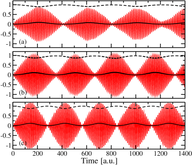
Figure 2: Dipole moment (red) and populations $n_{e}^{s}$ (solid black line) and $n_{g}^{s}$ (dashed black line) for ALDA (a) and EXX (b). The results from the theoretical model Eq. (16) are given in (c). The calculations in (a) were performed for $\omega^{ALDA}=0.476$ Ha and the ones in (b) and (c) for $\omega^{EXX}=0.549$ Ha.

Here, we employ two different approximations to the one-dimensional xc potential, the recently derived adiabatic local density approximation (ALDA) HFCVMTR2011 and exact exchange (EXX) which for a two-electron singlet is adiabatic and equal to Hartree-Fock. The resonant frequencies are calculated from linear response in octopus which yields $\omega^{ALDA}=0.476$ Ha and $\omega^{EXX}=0.549$ Ha. We then apply a laser field in analogy to the exact calculation with an amplitude of ${\cal E}_{0}=0.0125\omega$ using the resonant frequency for each case. Propagating with the ALDA and EXX results in the dipole moments shown in Fig. 2a and  2b respectively. Note that despite of the applied laser being in resonance with the system both EXX and ALDA approximations show the characteristic signature of detuned Rabi oscillations: the population of the excited state is incomplete and the zeros of the dipole moment coincide with the minima of $n_{e}^{s}$ but not with the minima of $n_{g}^{s}$, giving a similar picture as in Fig. 1b. As the KS system only has to reproduce the exact density, we do not expect a complete population of the excited KS orbital. However, as we can see from Fig. 2, the system remains mainly in its ground state and, like already pointed out in BauerRugg , its density resembles mostly the ground-state density. This does not imply that the KS system is not undergoing Rabi oscillations. Based on the behavior of the populations we postulate that the oscillations seen in Fig. 2 are in fact detuned Rabi oscillations and not of classical origin as claimed in BauerRugg .

If an adiabatic approximation is used the potential at time $t$ is a functional of the density at this time, i.e. $V_{hxc}(t)=V_{hxc}[\rho(t)]$. In the following, we show that $V_{hxc}(t)$ indeed introduces a detuning that drives the system out of resonance. We again rely on the conditions (2), i.e. describe the KS system as an effective two-level system with

$$\phi(t)({\bf r},t)=a_{g}^{s}(t)\phi_{g}({\bf r})+a_{e}^{s}(t)\phi_{e}({\bf r}).$$ (9)

Projecting the KS Hamiltonian (8) onto the two-level KS space (9) yields the $2\times 2$ matrix

$$\left({\begin{array}[]{cc}\epsilon_{g}^{s}+\epsilon_{g}^{xc}(t)&d_{eg}^{s}{\cal E}(t)+{\cal F}_{xc}(t)\\ d_{eg}^{s}{\cal E}(t)+{\cal F}_{xc}(t)&\epsilon_{e}^{s}+\epsilon_{e}^{xc}(t)\\ \end{array}}\right)$$ (10)

with the dipole matrix element being $d_{eg}^{s}=\langle\phi_{e}|\hat{{\bf r}}|\phi_{g}\rangle$. The additional terms, $\epsilon_{g,e}^{xc}(t)=\langle\phi_{g,e}|\hat{V}_{hxc}^{dyn}(t)|\phi_{g,e}\rangle$ and ${\cal F}_{xc}(t)=\langle\phi_{g}|\hat{V}_{hxc}^{dyn}(t)|\phi_{e}\rangle$, describe the fictitious time-dependence that results in a dynamical detuning of the Rabi oscillations. As in the linear Rabi oscillations, the matrix (10) determines the coefficients $a_{g}^{s}(t)$ and $a_{e}^{s}(t)$ and the equations of motion for the dipole moment $d^{s}(t)$ and the population $n_{e}^{s}(t)=|a_{e}^{s}(t)|^{2}$. Compared to Eq. (5) we note that each entry in (10) contains an additional term depending on $V_{hxc}^{dyn}$. In order to investigate the consequences of this term we again study the external potential (7) and use the EXX functional for which a relatively simple analytic expression for the additional matrix elements can be derived. The behavior using ALDA is very similar to the one for the EXX approximation (see Fig. 2a). The analysis, however, is more involved due to the functional not being linear in the density.

For the two-electron singlet case investigated here, the Hartree-exchange-correlation potential $V_{hxc}^{EXX}(x,t)$ is equal to half the Hartree potential and, hence, given as

$$V_{hxc}^{EXX}(x,t)=\frac{1}{2}\int d^{3}x\hat{V}_{ee}(|x-x^{\prime}|)(\rho_{0}(x^{\prime})+\delta\rho(x^{\prime},t)).$$ (11)

Here, the part containing $\rho_{0}$ determines $V_{hxc}[\rho_{0}]$ while $\delta\rho$ results in the additional $V_{hxc}^{dyn}$. We then rewrite the contributions to the diagonal terms of Eq. (10) as

$$\epsilon_{g}^{xc}(t)=\lambda_{g}n_{e}^{s}(t),\quad\epsilon_{e}^{xc}(t)=\lambda_{e}n_{e}^{s}(t)$$ (12)

where, in EXX, the coefficient $\lambda$ reads

$$\lambda_{g,e}\!=\!\int\!\!\!\!\int\!\!dx\>dx^{\prime}\left(|\phi_{e}(x^{\prime})|^{2}-|\phi_{g}(x^{\prime})|^{2}\right)\hat{V}_{ee}(|x-x^{\prime}|)|\phi_{g,e}(x)|^{2}.$$ (13)

For the off-diagonal contributions we recall that $d^{s}(t)=2d_{eg}^{s}Re[a_{g}^{s}(t)^{*}a_{e}^{s}(t)]$, as in the exact case, and rewrite the contribution of ${V}_{hxc}^{dyn}(t)$ to the off-diagonal terms as a coefficient $g$ multiplied by the time-dependent dipole moment

$${\cal F}_{xc}(t)=g\frac{d^{s}(t)}{d_{eg}^{s}}.$$ (14)

Here, g is given as

$$g=\int\!\!\!\!\int dxdx^{\prime}\phi_{e}(x^{\prime})\phi_{g}(x^{\prime})\hat{V}_{ee}(|x-x^{\prime}|)\phi_{g}(x)\phi_{e}(x).$$ (15)

The coefficient $g$ also enters when one calculates the resonant frequencies in linear response. Within the two-level approximation the resonant frequency is given as $\omega_{0}^{s}=\sqrt{\Delta_{s}(\Delta_{s}+2g)}$ (see Appendix B) which yields $\omega_{0}^{EXX}=0.532$ Ha. The deviation from $\omega^{EXX}$ calculated from time propagation of Hamiltonian (8) in octopus is of the order of $3\%$, coinciding with the deviation of our system from a true two-level system which we estimate from $\left(1-(n_{g}^{s}(t)+n_{e}^{s}(t))\right)$. Using again the RWA we obtain, to leading order in $\lambda/\omega_{0}$ and $g/\omega_{0}$, the following differential equation for the level population $n_{e}^{s}(t)$ (see Appendix B for the derivation)

$$\partial^{2}_{t}n_{e}^{s}(t)=-\left(\frac{\gamma^{2}}{2}n_{e}^{s}(t)^{2}+\Omega_{s}^{2}\right)n_{e}^{s}(t)+\frac{1}{2}\Omega_{s}^{2}$$ (16)

with $\Omega_{s}=d_{eg}^{s}{\cal E}_{0}$ and $\gamma=\lambda-2g$. Neglecting higher order terms leads to an error of about 10$\%$. Within these error bars we can safely use Eq. (16) because it contains all the relevant physics. Unlike Eq. (6) which represents a harmonic oscillator, Eq. (16) corresponds to an anharmonic quartic oscillator and its solution can be written in terms of Jacobi elliptic functions AQO . Equivalently, Eq. (16) can be integrated numerically. Comparing Eqs. (16) and (6) we conclude that the adiabatic approximation introduces a time-dependent detuning proportional to $\frac{1}{\sqrt{2}}\gamma n_{e}^{s}(t)$. The anharmonic oscillator no longer represents a parabola but the dynamical detuning also results in an increase of the restoring force. This can be clearly seen in Fig. 3 where we plot the potential corresponding to the restoring force in Eqs. (6) and (16) for the detunings of Fig. 1 and the EXX calculation( Fig. 2c).

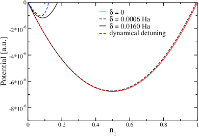
Figure 3: Potentials corresponding to the differential equations (6) and (16). The dynamical detuning leads to a quartic potential which has a similar effect to the potential as a large detuning in the applied frequency (see text for details).

Using the same 1D model system Eq. (7) as before we apply a field of amplitude ${\cal E}_{0}=0.0125\omega^{EXX}$ and calculate the dipole moment $d^{s}(t)$ and population $n_{e}^{s}(t)$ from Eq. (16). For this system we obtain for the bare KS eigenvalues $\epsilon_{g}^{s}=-0.750$ Ha and $\epsilon_{e}^{s}=-0.257$ Ha which yields $\Delta_{s}=0.494$ Ha. For the various matrix elements we obtain $d_{eg}^{s}=0.897$, $g=0.071$, $\lambda=-0.125$, and $\gamma=-0.268$. The results are shown in Fig. 2c in comparison to the numerically exact time-propagation in octopus (Fig. 2b). The discrepancy between the numerical propagation and the analytical results is mainly due to the fact that we kept only the leading orders in $\lambda/\omega_{0}$ and $g/\omega_{0}$ in the derivation of Eq. (16). However, our simple model clearly captures the effect of the dynamical detuning present in all adiabatic functionals. In the physical system the density changes dramatically during the transition and, in order to be able to describe resonant Rabi oscillations, a functional has to keep track of these changes over time, i.e. it needs to have memory. For any adiabatic functional the potential will change due to the changing density and the system is driven out of resonance. We emphasize that this effect is not limited to TDDFT but is generic for all mean-field theories, e.g. HF or all hybrids, when the effective potential depends instantaneously on the state of the system.

IV Conclusion

In conclusion, we demonstrate that the use of adiabatic approximations leads to a dynamical detuning in the description of Rabi oscillations. Only the inclusion of an appropriate memory dependence can correct the fictitious time-dependence of the resonant frequency. In particular, by clearly identifying the reason behind the failure of adiabatic approximations, we are able to prove the correspronding conjecture recently made in BauerRugg . Our results constitute a very stringent test for the development of new xc functionals beyond the linear regime as all (adiabatic) functionals available till now fail to reproduce Rabi dynamics. Adiabatic functionals will fail similarly in the description of all processes involving a change in the population of states. Work along the lines of deriving a new memory-dependent functional is ongoing. The description of photo-induced processes in chemistry, physics, and biology and the new field of attosecond electron dynamics and high-intense lasers all demand fundamental functional developments going beyond the adiabatic approximation.

Appendix A Equation of motion for $n_{e}(t)$ in the interacting many-body problem

We provide here a derivation of the equation of motion, Eq. (6), for the population $n_{e}(t)$ of the excited state.

As a first step we formulate a system of equations for physical observables, the dipole moment $d(t)=2d_{eg}Re[a_{g}^{*}a_{e}]$, the “transition current” $J(t)=2d_{eg}Im[a_{g}^{*}a_{e}]$, and the populations $n_{g,e}(t)=|a_{g,e}|^{2}$. Using the Schrödinger equation Eq. (5) for $a_{g,e}(t)$ and the above definitions of $d(t)$, $J(t)$ and $n_{g,e}(t)$ one can derive the following coupled differential equations for these quantities,

$$\partial_{t}d(t) = \Delta J(t),$$ (17)

$$\partial_{t}J(t) = -\Delta d(t)-2(n_{g}-n_{e})|d_{eg}|^{2}{\cal E}(t),$$ (18)

$$\partial_{t}n_{e}(t) = -J(t){\cal E}(t),$$ (19)

where $\Delta=\epsilon_{e}-\epsilon_{g}$ with $\epsilon_{g,e}=\langle\psi_{g,e}|\hat{H}(t)|\psi_{g,e}\rangle$ and $d_{eg}{\cal E}(t)=\langle\psi_{e}|\hat{H}(t)|\psi_{g}\rangle$. Equations (17), (18), and (19) correspond to the two-level version of the continuity equation, the equation of motion for the transition current, and the energy balance equation, respectively. These equation have to be supplemented with the normalization condition $n_{g}(t)+n_{e}(t)=1$, and the initial conditions $d(0)=J(0)=n_{e}(0)=0$.

By combining Eqs. (17) and (18) one obtains an equation of motion for the dipole moment $d(t)$

$$\partial^{2}_{t}d(t)=-\Delta^{2}d(t)-2(1-2n_{e})\Delta|d_{eg}|^{2}{\cal E}(t).$$ (20)

The next step in the derivation is to simplify this equation using RWA. Namely, we separate “fast” and “slow” time scales by writing the dipole moment in the following form

$$d(t)=d_{eg}[b_{1}(t)\cos(\omega t)+b_{2}(t)\sin(\omega t)]$$ (21)

where the coefficients $b_{1}(t)$ and $b_{2}(t)$ are assumed to be slowly varying ($\partial_{t}{b}/b\ll\omega=\Delta+\delta$). Inserting the ansatz of Eq. (21) into Eq. (20) and making use of the condition $\delta,\Omega_{0}<<\Delta$ we arrive at the system of first order differential equations for slow variables

$$\partial_{t}b_{2}(t)-\delta b_{1}(t) = 0$$ (22)

$$\partial_{t}b_{1}(t)+\delta b_{2}(t)-\Omega_{0}(1-2n_{e}) = 0$$ (23)

From Eqs. (19) and (17) we obtain the equation of motion for the populations

$$\partial_{t}n_{e}=\frac{1}{2}\Omega_{0}b_{1}(t).$$ (24)

where we again kept only leading in $\omega$ terms and, as usual in RWA, neglected irrelevant terms oscillating with $2\omega$. Combining this equation with Eq. (22) results in

$$\partial_{t}\left[b_{2}(t)-\frac{2\delta}{\Omega_{0}}n_{e}(t)\right]=0$$ (25)

which, together with the initial conditions $n_{e}(0)=0$ and $\partial_{t}d(0)=0$, yields

$$b_{2}(t)=\frac{2\delta}{\Omega_{0}}n_{e}(t)$$ (26)

and, due to Eq. (22),

$$b_{1}(t) = \frac{2}{\Omega_{0}}\partial_{t}n_{e}(t)$$ (27)

Finally, by inserting Eq. (26) and Eq. (27) into Eq. (23) we arrive at the differential equation Eq. (6) for the population $n_{e}(t)$ of the excited state in the many-body interacting system.

Appendix B Equation of motion for $n_{e}^{s}(t)$ in the KS system

Following the same scheme as in appendix A we do now derive Eq. (16) describing dynamics of the KS population $n_{e}^{s}(t)$. The equations of motion for the KS quantities, $d^{s}(t)=2d_{eg}^{s}Re[(a_{g}^{s})^{*}a_{e}^{s}]$, $J^{s}(t)=2d_{eg}^{s}Im[(a_{g}^{s})^{*}a_{e}^{s}]$, and $n_{g,e}^{s}(t)=|a_{g,e}^{s}|^{2}$ are similar to Eqs. (17)-(19) and can be obtained with the following replacements:$\Delta\rightarrow\Delta(t)=\Delta_{s}+\epsilon_{e}^{xc}(t)-\epsilon_{g}^{xc}(t)$, and $d_{eg}{\cal E}(t)\rightarrow d_{eg}^{s}{\cal E}(t)+{\cal F}_{xc}(t)$. One can again derive an equation of motion for the dipole moment (in analogy to Eq. (20)) which, due to the additional time dependence in $\Delta(t)$, aquires an additional term and reads

$$\begin{split}\partial^{2}_{t}{d^{s}(t)}=&-\Delta^{2}(t){d^{s}(t)}+\frac{\partial_{t}\Delta(t)}{\Delta(t)}{\partial_{t}d^{s}(t)}\\ &-2(n_{g}^{s}-n_{e}^{s})\Delta(t)d_{eg}(d_{eg}^{s}{\cal E}(t)+{\cal F}_{xc}(t)),\end{split}$$ (28)

where ${\cal F}_{xc}(t)$ is given by Eq. (14). For the two-electron singlet case and EXX approximation, the time-dependent contribution to the Hartree-exchange-correlation potential is proportional to $\delta\rho(x,t)$. As $\delta\rho(x,t)=2n_{e}^{s}(t)(|\phi_{e}(x)|^{2}-|\phi_{g}(x)|^{2})+2d^{s}(t)\phi_{g}(x)\phi_{e}(x)$ we obtain

$$\Delta(t)=\Delta_{s}+\lambda n_{e}^{s}(t)$$ (29)

with $\lambda=\lambda_{e}-\lambda_{g}$ and $\lambda_{g,e}$ defined in Eq. (13).

The resonant frequency $\omega_{0}^{EXX}$ is now not given by the KS energy difference $\Delta_{s}$ but needs to be calculated from the linear response. In the linear regime Eq. (28) reduces to the following form

$$\partial^{2}_{t}{d^{s}(t)}=-\Delta_{s}\left((\Delta_{s}+2g)d^{s}(t)-2\Delta_{s}|d_{eg}^{s}|^{2}{\cal E}(t)\right),$$ (30)

From the first term in the right hand side in Eq. (30) we identify the linear response resonant frequency as

$$\omega^{EXX}_{0}=\sqrt{(\Delta_{s}+2g)\Delta_{s}}.$$ (31)

We can now apply the same procedure to Eq. (28) as in the interacting case to derive an equation of motion for the occupation $n_{e}^{s}(t)$. Below, as well as in the main text, for the KS system we consider only the case of a resonant excitation, $\omega=\omega^{EXX}_{0}$, i. e. $\delta=0$. Employing the ansatz of Eq. (21) for the KS dipole moment $d^{s}(t)$, in analogy to Eqs. (22) and (23) we obtain

$$\partial_{t}b_{2}^{s}(t)+\left(\lambda-2g\right)n_{e}^{s}(t)b_{1}^{s}(t) = 0$$ (32)

$$\partial_{t}b_{1}^{s}(t)-\left(\lambda-2g\right)n_{e}^{s}(t)b_{2}^{s}(t)$$

$$-\Omega_{s}(1-2n_{e}^{s}(t)) = 0$$ (33)

with $\Omega_{s}=d_{eg}^{s}{\cal E}_{0}$. From the EXX analog of Eq. (19) (the energy balance equation) we find that to the leading order in RWA the equation of motion for the occupation has exactly the same form as Eq. (24), i. e.,

$$\partial_{t}n_{e}^{s}(t)=\frac{1}{2}\Omega_{s}b_{1}^{s}(t).$$ (34)

Therefore, with the initial conditions $n_{e}^{s}(0)=0$ and $\partial_{t}n_{e}^{s}(0)=0$ we get for the two coefficients

$$b_{1}^{s}(t) = \frac{2}{\Omega_{s}}\partial_{t}n_{e}^{s}(t),$$ (35)

$$b_{2}^{s}(t) = -\frac{\lambda-2g}{\Omega_{s}}(n_{e}^{s}(t))^{2}.$$ (36)

Finally, by inserting Eq. (35) and Eq. (36) into Eq. (33) we arrive at the differential equation Eq. (16) for the population $n_{e}^{s}(t)$ of the KS excited state.

References

- (1) E. Runge and E. K. U. Gross, Phys. Rev. Lett. 52, 997 (1984).
- (2) Time-Dependent Density Functional Theory, Vol. 706 of Lecture Notes in Physics, edited by M. Marques et al. (Springer, Berlin/Heidelberg, 2006).
- (3) M. Ruggenthaler and D. Bauer, Phys. Rev. Lett. 102, 233001 (2009).
- (4) N. T. Maitra, F. Zhang, R. Cave, and K. Burke, J. Chem. Phys. 120, 5932 (2004).
- (5) A. Dreuw and M. Head-Gordon, J. Am. Chem. Soc. 126, 4007 (2004).
- (6) M. Petersilka and E.K.U. Gross, Laser Physics 9, 1 (1999).
- (7) D. Tannor, Introduction to Quantum Mechanics a time-dependent perspective (University Science books, Sausalito, California, 2007), pp. 479–482.
- (8) N. Helbig, J. Fuks, M. Casula, M. Verstraete, M. Marques, I. Tokatly, A. Rubio, Phys. Rev. A 83, 032503 (2011).
- (9) A. Castro et al., Phys. Stat. Sol. (b) 243, 2465 (2006).
- (10) M. A. L. Marques, A. Castro, G. F. Bertsch, and A. Rubio, Comp. Phys. Comm. 151, 60 (2003).
- (11) A. Martin Sanchez, J. Diaz Bejarano, and D. Caceres Marzal, Journal of Sound and Vibration 161, 19 (1993).