Dynamic charge correlations near the Peierls transition

Abstract

The quantum phase transition between a repulsive Luttinger liquid and an insulating Peierls state is studied in the framework of the one-dimensional spinless Holstein model. We focus on the adiabatic regime but include the full quantum dynamics of the phonons. Using continuous-time quantum Monte Carlo simulations, we track in particular the dynamic charge structure factor and the single-particle spectrum across the transition. With increasing electron-phonon coupling, the dynamic charge structure factor reveals the emergence of a charge gap, and a clear signature of phonon softening at the zone boundary. The single-particle spectral function evolves continuously across the transition. Hybridization of the charge and phonon modes of the Luttinger liquid description leads to two modes, one of which corresponds to the coherent polaron band. This band acquires a gap upon entering the Peierls phase, whereas the other mode constitutes the incoherent, high-energy spectrum with backfolded shadow bands. Coherent polaronic motion is a direct consequence of quantum lattice fluctuations. In the strong-coupling regime, the spectrum is described by the static, mean-field limit. Importantly, whereas finite electron density in general leads to screening of polaron effects, the latter reappear at half filling due to charge ordering and lattice dimerization.

I Introduction

The Peierls transition is a hallmark feature of quasi-one-dimensional materials, such as conjugated polymers or organic charge-transfer salts. Peierls originally predicted a band insulator for any finite electron-phonon coupling for a half-filled system due to an instability in the presence of perfect nesting.Peierls (1955) A full understanding of the physics requires to account for both quantum lattice fluctuations and strong electronic correlations.Tsuda et al. (1990) For example, it has been found theoretically that quantum fluctuations of the lattice give rise to a metallic state below a finite critical coupling strength.Hirsch and Fradkin (1982)

A minimal yet rich theoretical setting studied is the spinless Holstein modelHolstein (1959) at half filling. With increasing electron-phonon coupling, a quantum phase transition from a metal to a Peierls insulator (PI) with charge-density-wave order occurs.Hirsch and Fradkin (1982, 1983) The phase diagram has been mapped out with high a accuracy.Bursill et al. (1998); Weiße and Fehske (1998); Jeckelmann et al. (1999); Hohenadler et al. (2006a) The character of the phase transition depends on the phonon frequency.Hohenadler et al. (2006a) In the adiabatic regime considered here, the Peierls state is a band insulator, and the transition is accompanied by the softening of the phonon mode at the zone boundary. The critical coupling is rather small, so that our Monte Carlo method becomes very efficient (see Sec. III). In the nonadiabatic regime, small polarons form a polaronic superlattice, and the bare phonon mode hardens on approaching the transition.Hohenadler et al. (2006a)

A metallic phase of one-dimensional spinless fermions is described by Luttinger liquid (LL) theory, with an interaction parameter $K_{\rho}$, even in the presence of a coupling to phonons.Haldane (1981); Meden et al. (1994) Until recently, from scaling analysis of the ground-state energy,McKenzie et al. (1996a); Fehske et al. (2000); Weiße et al. (2000) there was evidence for a crossover from an attractive LL ($K_{\rho}>1$) at low phonon frequencies, to a repulsive LL ($K_{\rho}<1$) at high phonon frequencies. However, large-scale density-matrix renormalization group (DMRG) calculations of the charge structure factor have revealed that the LL is always repulsive, i.e. $K_{\rho}\leq 1$.Ejima and Fehske (2009) The Peierls quantum phase transition in the spinless Holstein model is of the Kosterlitz-Thouless (KT) type for all values of the phonon frequency, with $K_{\rho}=1/2$ at the transition point.Ejima and Fehske (2009) The KT transition was previously known to occur in the nonadiabatic regime where the model can be mapped onto the $XXZ$ Hamiltonian.Hirsch and Fradkin (1982, 1983); Bursill et al. (1998) The suppression of superconducting correlations is ascribed to the spinless nature of the charge carriers, which prevents onsite pairing. In the spinful model at quarter filling, a transition from a LL to a (metallic) Luther-Emery liquid with finite spin gap but zero charge gap was discovered.Assaad (2008) An LL theory for gapless Peierls states has been developed.Voit (1998)

Given the continuous nature of the Peierls transition, one may argue that LL features should also survive at moderate couplings in the PI state, i.e. sufficiently close to the transition. Such a scenario will indeed emerge from our results for the single-particle spectral function, which reveal mixed charge and phonon modes (i.e., polarons) in both phases, with a finite single-particle gap in the Peierls phase. For the metallic phase, we shall compare to exact bosonization results for the spectral function.Meden et al. (1994)

Dynamic properties of the spinless Holstein model have been studied numerically and analytically,Hohenadler et al. (2003); Sykora et al. (2005); Hohenadler et al. (2005); Hohenadler et al. (2006b); Creffield et al. (2005); Wellein et al. (2006); Hohenadler et al. (2006a); Sykora et al. (2006a); Loos et al. (2006a, 2007) (we refer to these papers for a more comprehensive review of work on the spinless Holstein model) except for the dynamic charge structure factor. The spinless Holstein model may be considered as the strong-Hubbard-$U$ limit of the Hubbard-Holstein model, so that the formation of singlet bipolarons is suppressed. Away from half filling, it captures polaronic effects believed to be crucial in strongly correlated materials such as one-dimensional MX chains,Baeriswyl and Bishop (1987, 1988); Bishop and Swanson (1993) or quasi-two respectively three-dimensional manganites.Edwards (2002); Hohenadler and Edwards (2002); Hohenadler et al. (2005)

Here we apply an exact continuous-time quantum Monte Carlo (CTQMC) method to revisit the Peierls transition in the spinless Holstein model. Apart from presenting a highly non-trivial test of the method for lattice problems, we make several contributions to the understanding of the physics near the transition. In particular, we compute the dynamic charge structure factor, and relate the single-particle spectral function to LL theory and polaron physics on both sides of the transition, and to mean-field theory in the strong-coupling regime.

The paper is organized as follows. We introduce the model in Sec. II, and provide some details of the method for the present problem in Sec. III. A discussion of our results is given in Sec. IV, and we conclude in Sec. V.

II Model

The Hamiltonian $\hat{H}=\hat{H}_{0}+\hat{H}_{1}$ takes the form

$$\hat{H}_{0} =-t\sum_{\langle ij\rangle}\left(c^{\dagger}_{i}c^{\phantom{{\dagger}}}_{j}+\text{H.c.}\right)-\mu\sum_{i}\hat{n}_{i}\,,$$ (1)

$$\hat{H}_{1} =\sum_{i}\left(\frac{1}{2M}\hat{P}_{i}^{2}+\frac{K}{2}\hat{Q}_{i}^{2}\right)-\gamma\sum_{i}\hat{Q}_{i}(\hat{n}_{i}-\mbox{$\frac{1}{2}$})\,.$$

The first term $\hat{H}_{0}$ describes hopping of spinless fermions between neighboring sites with overlap integral $t$ and free dispersion $\epsilon(q)=-2t\cos q$, $\mu$ is the chemical potential, and the charge density operator is defined as $\hat{n}_{i}=c^{\dagger}_{i}c^{\phantom{{\dagger}}}_{i}$ with eigenvalues 0, 1. The first part of $\hat{H}_{1}$ describes the free dynamics of the lattice in the harmonic approximation; $\omega_{0}$ is the phonon frequency, and $K=\omega_{0}^{2}M$. The second part couples the electron density to the lattice displacement. The half filled band (density $n=0.5$) corresponds to $\mu=0$, and we work in one dimension.

Due to the use of first quantization (more convenient for the present method), the notation, in particular the coupling $\gamma$, differs from that used in previous work we shall compare to,Hohenadler et al. (2006a); Sykora et al. (2005) where the coupling term is written in the form $-g\omega_{0}\sum_{i}(b^{\dagger}_{i}+b^{\phantom{{\dagger}}}_{i})(\hat{n}_{i}-\mbox{$\frac{1}{2}$})$. To reconcile the two notations, we use the dimensionless coupling constant $\lambda=2\varepsilon_{\text{p}}/W$, where $\varepsilon_{\text{p}}$ is the polaron binding energy, and $W=4t$ is the bandwidth; $\lambda$ is the relevant dimensionless ratio in the adiabatic regime $\omega_{0}<t$, separating weak ($\lambda\ll 1$) and strong coupling ($\lambda\gg 1$); small-polaron formation occurs at $\lambda\simeq 1$.De Raedt and Lagendijk (1982) In terms of $g$ we have $\varepsilon_{\text{p}}=g^{2}\omega_{0}$ and $\lambda=g^{2}\omega_{0}/(2t)$, whereas in terms of $\gamma$ the relations are $\varepsilon_{\text{p}}=\gamma^{2}/(2K)=\gamma^{2}/(2\omega_{0}^{2})$ and $\lambda=\gamma^{2}/(\omega_{0}^{2}W)$. We use $t$ as the unit of energy, and set $\hbar=k_{\text{B}}=M=1$.

III Method

The CTQMC is based on an exact diagrammatic expansion of the partition function around the non-interacting limit;Rubtsov et al. (2005) the expansion converges for any finite fermionic system at finite temperature. The fact that Wick's theorem holds for each configuration allows for a simple calculation of one and two-particle fermionic Green's functions. As discussed elsewhere,Rubtsov et al. (2005); Assaad and Lang (2007) updates take the form of the addition and removal of single vertices, and optionally flipping Ising spins. The method is exact also for strong coupling, but becomes numerically less efficient due to large matrix sizes. The numerical effort scales with the cube of the average expansion order; the latter depends linearly on the system size $N$, inverse temperature $\beta=1/T$ and (effective) coupling strength.

The extension of the CTQMC method to electron-phonon problems has been discussed before.Assaad and Lang (2007) Most importantly, as the algorithm is action based,Rubtsov et al. (2005) the path integral over the phonon degrees of freedom can be performed exactly for a wide range of problemsFeynman (1955) (see also Ref. Assaad and Lang, 2007). This leads to a retarded electron-electron interaction of the form

$$S_{1}=-\int_{0}^{\beta}\int_{0}^{\beta}d\tau d\tau^{\prime}\sum_{i}[n_{i}(\tau)-\mbox{$\frac{1}{2}$}]D(\tau-\tau^{\prime})[n_{i}(\tau^{\prime})-\mbox{$\frac{1}{2}$}]\,,$$ (2)

where $D(\tau)$ is the phonon propagator of the Holstein model [diagonal in real-space due to the onsite interaction in Eq. (1)], and $n_{i}(\tau)$ is a Grassmann bilinear. The result is a purely fermionic algorithm, with no additional sampling of phonon degrees of freedom. The vertices have equal real space coordinates but in general different times $\tau,\tau^{\prime}$, distributed $\sim D(\tau-\tau^{\prime})$. The range of the retarded interaction along the imaginary time is of the order $1/\omega_{0}$, but we find the algorithm to be efficient even for small $\omega_{0}$. The weight to add a vertex is proportional to $\lambda\beta N$. In the present case, the spinless nature of the model makes only one spin direction appear in the algorithm. There is no sign problem, and we consider system sizes $N=4l+2$ with periodic boundary conditions.

Compared to previous QMC studies of the spinless Holstein model,Hirsch and Fradkin (1982, 1983); McKenzie et al. (1996b); Hohenadler et al. (2005); Creffield et al. (2005) the CTQMC algorithm is free of errors associated with a Trotter discretization. There is also no cutoff for the phonon Hilbert space, as the lattice degrees of freedom are integrated out exactly.

Two key quantities for studying the Peierls transition are the static charge structure factor

$$S_{\rho}(q)=\sum_{r}\left(\langle\hat{n}_{r}\hat{n}_{0}\rangle-\langle\hat{n}_{r}\rangle\langle\hat{n}_{0}\rangle\right)e^{iqr}\,,$$ (3)

and the dynamic charge structure factor given in the Lehmann representation as

$$S_{\rho}(q,\omega)=\frac{1}{Z}\sum_{mn} {|\left\langle n\right|\hat{\rho}_{q}\left|m\right\rangle|}^{2}e^{-\beta E_{m}}$$

$$\times\delta(E_{m}-E_{n}-\omega)\,,$$ (4)

where $\left|n\right\rangle$ is an eigenstate with energy $E_{n}$, and we have defined $\hat{\rho}_{q}=\sum_{r}e^{iqr}(\hat{n}_{r}-\langle\hat{n}_{r}\rangle)/\sqrt{N}$.

We also consider the single-particle spectral function,

$$A(q,\omega)=\frac{1}{Z}\sum_{mn} {|\left\langle n\right|c_{q}\left|m\right\rangle|}^{2}(e^{-\beta E_{n}}+e^{-\beta E_{m}})$$

$$\times\delta(E_{m}-E_{n}-\omega)\,.$$ (5)

For the continuation from imaginary time to real frequencies, we use the stochastic Maximum Entropy method.Beach (unpublished)

IV Results

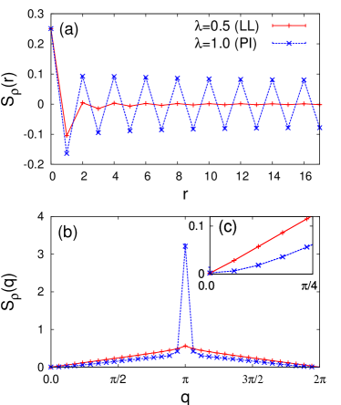
Figure 1: (Color online) Density-density correlations $S_{\rho}(r)=\langle\hat{n}_{r}\hat{n}_{0}\rangle$ (a) and charge structure factor (b). The coupling $\lambda=0.5$ corresponds to the metallic Luttinger liquid (LL) phase, whereas $\lambda=1.0$ is in the insulating Peierls phase (PI). (c) Closeup of (b). Here $\beta t=N=34$, $\omega_{0}=0.4t$ and $n=0.5$ (half filling). Lines are guides for the eye.

We anchor our choice of parameters to previous work,Sykora et al. (2005); Hohenadler et al. (2006a) focusing on the adiabatic regime $\omega_{0}<\ t$ (typically realized in experiments) where the Peierls transition falls into the weak or intermediate coupling regime. In the latter, the CTQMC is by its nature particularly efficient due to low average expansion orders. Explicitly, following Ref. Hohenadler et al., 2006a, we take $\omega_{0}=0.4t$. We mainly consider two characteristic values of the coupling strength, namely $\lambda=0.5$ and 1 (equivalent to $g^{2}=2.5$ respectively $5$). The latter lie just above and below the Peierls transition, see Fig. 1 in Ref. Hohenadler et al., 2006a, with the critical coupling known from DMRG calculationsHohenadler et al. (2006a) as $\lambda_{\text{c}}\approx 0.7$ ($g_{\text{c}}^{2}\approx 3.5$). The same parameters have been considered in Refs. Hohenadler et al., 2005; Wellein et al., 2006; Sykora et al., 2006a. We shall also compare to the case $\omega_{0}=0.1t$ considered in Ref. Sykora et al., 2005, for which $\lambda_{\text{c}}\approx 0.4$. The inverse temperature is set to $\beta t=N$.

IV.1 Static charge correlations

In Fig. 1(a) we show the density-density correlator $S_{\rho}(r)=\langle\hat{n}_{r}\hat{n}_{0}\rangle$. The $T=0$ bosonization result isGiamarchi (2004)

$$\langle\hat{n}_{x}\hat{n}_{0}\rangle=-\frac{K_{\rho}}{2\pi^{2}x^{2}}+\frac{A}{x^{2K_{\rho}}}\cos(2k_{\text{F}}x)\,,$$ (6)

with $k_{\text{F}}=n\pi$ for the spinless case, equal to $\pi/2$ for half filling. In the metallic phase, the LL parameter can be extracted from

$$K_{\rho}=2\pi\lim_{q\to 0}S_{\rho}(q)/q\,.$$ (7)

For simplicity, we take $K_{\rho}\approx 2\pi S_{\rho}(q_{1})/q_{1}$, where $q_{1}$ is the smallest nonzero wavevector for a given lattice size.

In the metallic LL phase, the amplitude of density correlations shows a power-law decay in real space. Since $K_{\rho}=0.96(1)<1$ for $\lambda=0.5$, we see a cusp in $S_{\rho}(q)$ at $q=2k_{\text{F}}$. The linear form of $S_{\rho}(q)$ at small $q$ [Fig. 1(c)] is evidence for a metallic state at $\lambda=0.5$.

In the Peierls phase ($\lambda=1$), the density correlation functions display long-range order (a charge density wave with one fermion on every other site, and a staggered lattice displacement with periodicity $\pi$). The small-$q$ behavior of $S_{\rho}(q)$ becomes nonlinear, see Fig. 1(c). Via the continuity equation, the long-wavelength limit of $S_{\rho}(q)$ can be directly related to the Drude part of the optical conductivity,Assaad (2008) and the absence of linear behavior of $S_{\rho}(q)$ as $q\to 0$ is equivalent to a vanishing Drude weight in the insulating Peierls state. As a result of long-range charge-density-wave order, $S_{\rho}(q)$ diverges with system size at $q=\pi=2k_{\text{F}}$, and serves as an order parameter. The Peierls state is quickly suppressed away from the commensurate density $n=0.5$.Hohenadler et al. (2007)

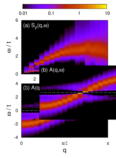
Figure 2: (Color online) (a) Dynamic charge structure factor $S_{\rho}(q,\omega)$ and (b) single-particle spectral function $A(q,\omega)$ in the metallic LL phase. Horizontal lines indicate (a) the bare phonon frequency $\omega_{0}$ and (b) the chemical potential $\mu=0$ (long dash) and $\pm\omega_{0}$ (short dash). We have limited the intensity range to reveal the subdominant features; the full range for (a) is shown in Fig. 6(b); for (b) see also Fig. 3. Parameters are $\omega_{0}=0.4t$, $\lambda=0.5$, and $\beta t=N=34$.

The LL parameter $K_{\rho}$ has been calculated as a function of $g$ with high accuracy in a large-scale DMRG study including finite-size scaling with up to 256 sites.Ejima and Fehske (2009) As the CTQMC is not capable of studying such large systems, and due to the additional complication of finite temperatures in our method [Eqs. (6) and (7) only hold at $T=0$] we do not attempt a quantitative comparison here. Instead, we have checked for both $\omega_{0}=1$ and $0.1$ that even on small systems ($N=22$) the CTQMC correctly reproduces $K_{\rho}\leq 1$ (repulsive LL), albeit with significant finite-size effects near $g_{\text{c}}$ as expected for a KT phase transition.Ejima and Fehske (2009)

IV.2 Excitation spectra in the metallic phase

We now turn to the discussion of the dynamical correlation functions, namely the dynamic charge structure factor and the single-particle spectral function. To our knowledge, the former has not been calculated for the present model before. In all intensity plots, we have refrained from using any kind of interpolation. This makes the limited (yet significantly higher than in previous numerical work) momentum resolution well discernible. The energy resolution was taken to be $0.01t$ or better.

The spectra in the LL phase ($\lambda=0.5$) are shown in Fig. 2. The dynamic charge structure factor $S_{\rho}(q,\omega)$ [Fig. 2(a)] shows the familiar continuum of particle-hole excitations of fermions in one dimension. At long wavelengths, we have a linear, gapless mode with dispersion $N(q,\omega)\approx N(q)\delta(\omega-v_{\rho}q)$ expected for the metallic phase. Near the zone boundary, the width of the continuum approaches the bare bandwidth $W=4t$. In addition, because of the coupling between the electron density and the phonons in the Hamiltonian (1), a signature of the renormalized optical phonon mode is visible at low energies. Already below the Peierls transition at $\lambda_{\text{c}}\approx 0.7$, it shows partial softening near $q=\pi$. Our findings are in excellent agreement with previous calculations of the phonon spectral function,Hohenadler et al. (2006a); Sykora et al. (2006b) see also Figs. 6(a) and (b) discussed below. Hence, despite the nondispersive nature of the Einstein phonons in Eq. (1) the coupling gives rise to a momentum dependence of the renormalized phonon frequency.

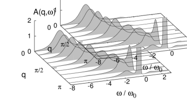
Figure 3: (Color online) Single-particle spectral function $A(q,\omega)$ in the metallic LL phase. Parameters as in Fig. 2(b).

The single-particle spectrum $A(q,\omega)$ in the LL phase [Fig. 2(b)] reveals a dominant band (note the logarithmic scale in all our intensity plots) closely tracking the cosine dispersion of the noninteracting problem, $\epsilon(q)$. Close to the Fermi level, inside the coherent interval $\omega\in[-\omega_{0},\omega_{0}]$, the main peak becomes noticeably sharper.Loos et al. (2006a) As noted previously,Meden et al. (1994); Hohenadler et al. (2006a); Sykora et al. (2005) the incoherent part ($|\omega|\geq\omega_{0}$) of the spectrum is broadened due to multiphonon processes;Loos et al. (2006a) the width is roughly $g^{2}=2.5$.

As expected, but not discussed in the numerical literatureSykora et al. (2005); Hohenadler et al. (2006a) (where the spectra are mostly interpreted in terms of polaron theory), the spectrum shares the main features of the exact bosonization result for a linear fermion dispersion.Meden et al. (1994) For comparison, we show the results in Fig. 2(b) again in Fig. 3 using a representation similar to that in Ref. Meden et al., 1994. The bare charge and phonon modes of the LL Hamiltonian of the spinless model hybridize and broaden; see also Ref. Assaad, 2008. This is equivalent to the formation of coherent polaronic quasiparticles, i.e. electrons dressed with phonons, with increased effective mass. At $k_{\text{F}}=\pi/2$ (we focus on $\omega<0$), there is a dominant zero-energy peak and a phonon satellite with threshold energy $-\omega_{0}$ whose width depends on the coupling strength. With $q$ moving away from $k_{\text{F}}$, spectral weight is transferred to the ``phonon peak'' (in the nomenclature of Meden et al. Meden et al. (1994)) which eventually becomes the dominant excitation and follows $\epsilon(q)$. Since in contrast to Ref. Meden et al., 1994 the bandwidth $W\gg\omega_{0}$, we observe multiple phonon satellites which merge into a broad band. This picture is consistent with previous numericalSykora et al. (2005); Hohenadler et al. (2006a) and analytical resultsSykora et al. (2006a) (though difficult to see in the latter) in the metallic phase. Similar results and an explicit comparison to LL theory have been reported for the spinful case.Assaad (2008)

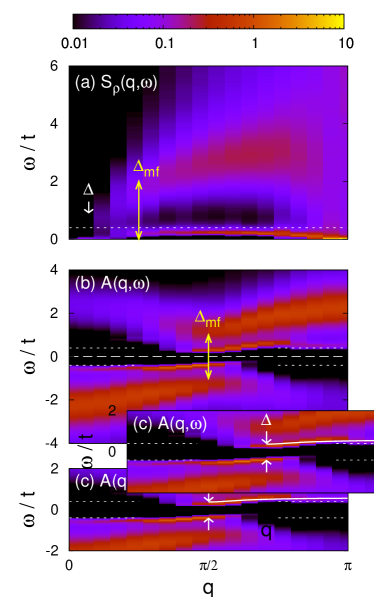
Figure 4: (Color online) (a) Dynamic charge structure factor $S_{\rho}(q,\omega)$ and (b) single-particle spectral function $A(q,\omega)$ in the Peierls phase. (c) Closeup of (b). Horizontal lines indicate (a) the bare phonon frequency $\omega_{0}$, (b) the chemical potential $\mu=0$ (long dashed) and $\pm\omega_{0}$ (short dashed), and (c) $\pm\omega_{0}$. The solid line in (c) is the shifted single-polaron band dispersion $\epsilon_{\text{p}}(q)+\Delta/2$ for the same parameters,Loos et al. (2006b) mapped from $[0,\pi]$ to $[k_{\text{F}},\pi]$ to facilitate comparison with half filling. The double-headed arrows in (a) and (b) designate the mean-field gap $\Delta_{\text{mf}}=\varepsilon_{\text{p}}=2t$. The single-headed arrows in (a) and (c) indicate the Peierls gap $\Delta\approx 0.75t$. In (a) we have limited the intensity range to reveal the subdominant features; the full range is shown in Fig. 6(c). Parameters are $\omega_{0}=0.4t$, $\lambda=1.0$, and $\beta t=N=34$.

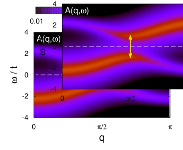
Figure 5: (Color online) Mean-field result for the single-particle spectrum $A(q,\omega)$ of the adiabatic ($\omega_{0}=0$), spinless Holstein model at $T=0$. Here $\Delta_{\text{mf}}=2t$ (arrow); we have replaced the $\delta$ peaks by Lorentzians with scaling parameter $0.3t$.

IV.3 Excitation spectra in the Peierls phase

In Fig. 4 we report the dynamic charge structure factor and the single-particle spectrum in the Peierls state, at $\lambda=1$. Mean-field results for $A(q,\omega)$ to be compared to Fig. 4(b) are shown in Fig. 5.

In the case of $S_{\rho}(q,\omega)$, see Fig. 4(a), we note that almost the entire spectral weight is located close to $\omega=0$, $q=\pi$. All other features, including the particle-hole continuum, have a spectral weight that is at least an order of magnitude lower (see caption). The accumulation of spectral weight at $\omega=0$, $q=\pi=2k_{\text{F}}$ is a result of the complete softening of the renormalized phonon dispersion and is characteristic of the displacive Peierls transition.Hohenadler et al. (2006a)

The renormalization of the phonon mode with increasing $\lambda$ is well visible in Fig. 6, which shows the low-energy range of $S_{\rho}(q,\omega)$ on a larger scale. Already for $\lambda=0.25$ [Fig. 6(a)] a partial softening is visible close to $q=\pi$. This trend continues with increasing $\lambda$, until the phonon has become gapless at $q=\pi$ in the Peierls state [Fig. 6(c)]. The softening scenario agrees well with previous work.Hohenadler et al. (2006a); Creffield et al. (2005); Sykora et al. (2005, 2006a) From $S_{\rho}(q,\omega)$ we cannot detect the previously reported splitting of the phonon mode into two branches, one of which hardens toward $\omega_{0}$ with increasing $\lambda$;Hohenadler et al. (2006a); Creffield et al. (2005) this may be a result of the very small spectral weight of the upper branch in the adiabatic regime.

The linear long-wavelength mode characteristic of the metallic phase [Fig. 2(a)] is completely suppressed with increasing $\lambda$, see Fig. 6. From Fig. 4(a), we can infer a gap of about $0.75t$ (left arrow) above which the particle-hole continuum starts. However, we can also estimate a second characteristic energy of about $2t$ (right arrow) where the spectral weight of the continuum increases noticeably. These two energy scales are related to the single-particle spectrum below. Our results for the dynamic charge structure factor are in accordance with previous calculations of the phonon spectral function for the present model.Hohenadler et al. (2006a); Sykora et al. (2006a) By comparison, the Luther-Emery phase of the spinful Holstein model is characterized by a soft phonon mode in addition to the particle-hole continuum which remains gapless for $q\to 0$.Assaad (2008)

The single-particle spectral function in the Peierls state is shown in Fig. 4(b). As hinted at by the results for $S_{\rho}(q,\omega)$, it is found to consist of two sets of features. There is a main, high-energy band that follows the free dispersion far away from $k_{\text{F}}$, and is split by the mean-field gap (see below) $\Delta_{\text{mf}}\approx\varepsilon_{\text{p}}=2t$ (indicated by the arrow). This value agrees with the gap $2t$ discussed above. The main band also reveals backfolded shadow bands for $q>k_{\text{F}}$ and $\omega<\omega_{0}$ respectively for $q<k_{\text{F}}$ and $\omega>\omega_{0}$. Additionally, within the mean-field gap, we have dispersive low-energy modes with a smaller gap $\Delta\approx 0.75t$ at $k_{\text{F}}$. We refer to this actual gap (determining the low-energy properties of the system) as the Peierls gap.

To first understand the high-energy features of $A(q,\omega)$, we consider the adiabatic limit $\omega_{0}=0$ of the spinless Holstein model,Hirsch and Fradkin (1983)

$$\hat{H}^{\prime}=\hat{H}_{0}-\mbox{$\frac{1}{2}$}K\sum_{i}Q_{i}^{2}-\gamma\sum_{i}Q_{i}(\hat{n}_{i}-\mbox{$\frac{1}{2}$})\,.$$ (8)

With the mean-field ansatz $Q_{i}=(-1)^{i}\xi$, we obtain the bands $E_{\pm}(q)=\pm[\epsilon(q)^{2}+\Delta_{\text{mf}}^{2}/4]^{1/2}$ with a gap $\Delta_{\text{mf}}$ at $k_{\text{F}}=\pi/2$. The mean-field gap is related to the lattice order parameter, $\Delta_{\text{mf}}\sim\xi^{2}$, and as for displaced oscillator states the lattice shift on occupied sites is $\xi\sim\sqrt{\varepsilon_{\text{p}}}$ so that we expect $\Delta_{\text{mf}}\sim\varepsilon_{\text{p}}$, in agreement with the QMC results. Rather than solving the gap equation, we simply set $\Delta_{\text{mf}}$ equal to the gap in our numerical data.

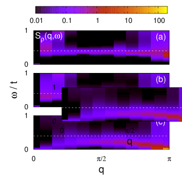
Figure 6: (Color online) Dynamic charge structure factor $S_{\rho}(q,\omega)$ at low energies. Horizontal lines indicate the bare phonon frequency $\omega_{0}$. Here $\omega_{0}=0.4t$, $\beta t=N=22$ and (a) $\lambda=0.25$ (LL), (b) $\lambda=0.5$ (LL), and (c) $\lambda=1$ (PI).

The resulting single-particle spectral functionVoit et al. (2000) contains two branches following $E_{\pm}(q)$, centered around $q=0$ respectively $\pi$, with spectral weights $w_{\pm}(q)=[1\pm\epsilon(q)/|E_{\pm}(q)|]/2$, and is shown in Fig. 5. Setting $\Delta_{\text{mf}}=\varepsilon_{\text{p}}$ and replacing the $\delta$ functions by Lorentzians with scaling parameter $0.3t$, we find excellent agreement with the high-energy features in Fig. 4(b). In particular, the backfolded shadow bands (including the $q$-dependence of the spectral weight) emerge as a natural feature of gapped systems with competing periodic potentials.Voit et al. (2000) The fact that the high-energy features of the quantum case $\omega_{0}>0$ are well captured by mean-field theory justifies the notation $\Delta_{\text{mf}}$ introduced above.

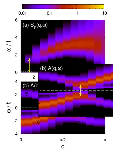
Figure 7: (Color online) (a) Dynamic charge structure factor $S_{\rho}(q,\omega)$ and (b) single-particle spectral function $A(q,\omega)$ in the Peierls phase. Horizontal lines indicate (a) the bare phonon frequency $\omega_{0}$, (b) the chemical potential $\mu=0$. Arrows designate the mean-field gap $\Delta_{\text{mf}}=\varepsilon_{\text{p}}=1.6t$. In (a), we have limited the intensity range to reveal the subdominant features. Parameters are $\omega_{0}=0.1t$, $\lambda=0.8$, and $\beta t=N=22$.

Let us now focus on the low-energy features inside the mean-field gap [Fig. 4(c)]. The absence of the latter in the mean-field results for the static limit suggests that they are related to quantum phonon fluctuations. Indeed, a particle added to the half-filled Peierls state [as described by $A(q\geq k_{\text{F}},\omega\geq 0)$, cf. Eq. (III)] is enabled by lattice fluctuations to propagate as a polaron. For the present parameters, the dimerization of the lattice opens a small but finite gap $\Delta\ll\Delta_{\text{mf}}$ in the corresponding polaronic band. Support for this picture comes from several directions. First, the width of the polaron bands in Fig. 4(c) is about 0.2t, in excellent agreement with the single-polaron results for the same parameters.Hohenadler et al. (2007) It also shows the well known flattening of the dispersion with increasing $q$.Wellein and Fehske (1997); Hohenadler et al. (2003) To demonstrate this agreement, we include in Fig. 4(c) the band dispersion $\epsilon_{\text{p}}(q)$ of a single polaron for the same parameters.Loos et al. (2006b) To compare to half filling, we shift the dispersion by $\Delta/2$, and map it from $[0,\pi]$ to $[k_{\text{F}},\pi]$. This yields excellent agreement for all $q$. Second, these bands have large electronic spectral weight near $q=k_{\text{F}}$ (corresponding to $q=0$ for a single polaron) but very small weight far away from $k_{\text{F}}$; the character of the coherent quasi-particle changes from electronic to phononic when the band energy intersects the bare phonon frequency,Wellein and Fehske (1997); Hohenadler et al. (2003) see also Fig. 3. Third, the energy gap $\Delta$ of the polaron bands, which is a property of the many-particle Peierls state, matches the corresponding excitation in the phonon spectral function for the same parameters,Hohenadler et al. (2006a) and agrees well with the phonon signature in Fig. 6(c) near $q=\pi/2$. For a single polaron, no phonon renormalization occurs, and the polaron band dispersion is clearly visible in the phonon spectral function.Loos et al. (2006b) The spectral function for the same parameters as Fig. 4 has been calculated by cluster perturbation theory.Hohenadler et al. (2006a) Whereas the polaron bands are difficult to identify in these approximate results, their signature inside the mean-field gap is clearly visible in the exact density of states.Wellein et al. (2006) The QMC results are in excellent agreement with the $T=0$ wavevector-resolved spectral function for these parameters obtained by exact diagonalization.Wellein (private communication) An alternative explanation for the polaron bands in terms of thermal excitations based on QMC simulations at much higher temperature was given before.Hohenadler et al. (2005) Polaron bands inside the static mean-field gap were also predicted analytically,Brazovskii (1978) and may be related to soliton excitations.Heeger et al. (1998)

From LL theory, the existence of the low-energy polaron modes is a necessary consequence of the continuous nature of the Peierls transition. The hybridized charge and phonon modes of the metallic phase evolve continuously with the coupling strength $\lambda$. One of the resulting two modes represents the backfolded high-energy band, whereas the other mode is the polaron band. This structure is already visible in the LL phase, see Figs. 2(b) and 3. The Peierls gap $\Delta$ in the polaron band opens exponentially slowly at the KT transition.

In the light of previous work on many-polaron systems, the validity of the single-polaron picture at half filling is not obvious. Away from half filling, the spinless Holstein model is metallic, and the overlap of the (extended) lattice distortions of individual carriers has been found to lead to a renormalization toward weak coupling and a loss of polaronic signatures.Hohenadler et al. (2005); Loos et al. (2006a); Hohenadler et al. (2007) However, the electrons constituting the insulating Peierls state are ordered in the dimerized lattice potential. Hence, an additional particle or hole does not undergo screening and behaves as a polaron, which moves in a dimerized but fluctuating potential. The most obvious impact of this Peierls background is the opening of the gap $\Delta$.

To complete the understanding of the dynamic charge correlations, we consider the strong-coupling regime. From single-polaron theory, we expect a strong reduction of the polaron bandwidth and the electronic spectral weight; the latter also becomes almost independent of $q$.Wellein and Fehske (1997); Hohenadler et al. (2003) The many-body Peierls gap $\Delta$ should increase with increasing dimerization ($\sim\sqrt{\Delta}$) of the lattice compared to phonon fluctuations ($\sim\sqrt{\omega_{0}}$), leading to a suppression of the coherent polaron motion.

Exact $T=0$ results for the single-particle spectrum in the Peierls phase have been reported by Sykora et al.,Sykora et al. (2005) for $N=8$, $\omega_{0}=0.1t$ and $\lambda=0.8$. On the linear scale of their Fig. 4, no features of the kind discussed here are visible. These results fall into the strong-coupling regime with respect to the Peierls transition, $\lambda\approx 2\lambda_{\text{c}}$. In particular, the mean-field gap $\Delta_{\text{mf}}\gg\omega_{0}$. As demonstrated by the QMC results for the parameters of Sykora et al. Sykora et al. (2005) shown in Fig. 7(b), the spectral weight of the polaron band is extremely small. At $k_{\text{F}}$, the gap $\Delta$ almost coincides with the mean-field gap $\Delta_{\text{mf}}$. The spectrum is dominated by the mean-field features of Fig. 5. As a result, the dynamic charge structure factor in Fig. 7(a) reveals only one energy scale ($\Delta_{\text{mf}}\approx\Delta$) for the onset of the particle-hole continuum, in addition to the signatures of phonon softening at low energies. A similar result is expected for $\omega_{0}=0.4t$ at much stronger coupling where the CTQMC method becomes inefficient.

Finally, the features of the spectral function in the Peierls state discussed here are specific to the adiabatic regime $\omega_{0}<t$. In the nonadiabatic case $\omega_{0}\gg t$, the critical coupling for the Peierls transition is large, so that electrons become heavy, small polarons already below $\lambda_{\text{c}}$.Hohenadler et al. (2006a) The corresponding polaron bands are extremely narrow and have very small electronic spectral weight.Wellein and Fehske (1997); Hohenadler et al. (2003) Similarly, the dispersion of the high-energy features is also substantially reduced.

V Conclusions

We have applied the exact continuous-time Monte Carlo method to the spinless Holstein model in the adiabatic regime. We find that the method is well suited to study the Peierls metal-insulator transition on the lattice. We have complemented previous work by computing the dynamic charge structure factor, and showing that is allows to track the softening of the phonon mode and the appearance of a charge gap with increasing electron-phonon coupling. For the single-particle spectral function, we explicitly demonstrated that the mixed charge and phonon modes of Luttinger liquid theory constitute the spectrum both below and above the Peierls transition. Most importantly, the spectrum in the Peierls phase consists in general of high-energy features readily understood in the static limit, and gapped low-energy polaron bands originating from quantum lattice fluctuations. These modes disappear in the strong-coupling regime. Our findings reconcile and unify previous and present results with both polaron theory and Luttinger liquid theory.

The spinless Holstein model captures two essential consequences of electron-phonon coupling, namely the formation of polarons (dressed quasi-particles) and the Peierls metal-insulator transition at commensurate filling. For any finite electron-phonon coupling, the electrons acquire some polaronic character. Based on this and previous work, we can conclude that starting from the low-density limit the well-defined polaron signatures known from the single-electron caseHohenadler et al. (2003) first become washed out with increasing density in the metallic phase.Hohenadler et al. (2007) However, once we approach the Peierls phase at half filling, mutual screening is strongly suppressed due to charge order and lattice dimerization, and clear polaron signatures reappear in the single-particle spectrum.