The unified picture for the classical laws of Batschinski and the rectilinear diameter for molecular fluids

Abstract

The explicit relations between the thermodynamic functions of the Lattice Gas model and the fluid within the framework of approach proposed earlier in [V. L. Kulinskii, J. Phys. Chem. B 114 2852 (2010)] are derived. It is shown that the Widom line serves as the natural border between the gas-like and the liquid-like states of the fluid. The explanation of the global cubic form of the binodal for the molecular liquids is proposed and the estimate for the amplitude of the binodal opening is obtained.

I Introduction

There are two classical laws for the molecular liquids known more than a century. Long time they were considered as mere curious facts restricted to the simple van der Waals equation of state (vdW EoS). First of them is the law of the rectilinear diameter (LRD) Cailletet and Mathias (1886); *crit_diam1_young_philmag1900; *crit_diambenzene_physrev1900; Guggenheim (1945). It states that the diameter of the coexistence curve in terms of density-temperature is the straight line:

$$\tilde{n}_{d}=\frac{n_{l}+n_{g}}{2n_{c}}=1+A\,\frac{T_{c}-T}{T_{c}}\,\,\,,\quad A>0$$ (1)

where $n_{i},\,i=l,g$ are the densities of the liquid and the gas phases correspondingly, $n_{c}$ is the critical density, $T$ is the temperature. Further we put the Boltzmann constant to unit: $k_{B}=1$. Another simple linear relation is the Batschinski law Batschinski (1906) for the vdW EoS:

$$P=\frac{n\,T}{1-n\,b}-a\,n^{2}\,,$$ (2)

where $P$ - is the pressure. It states that the line determined by the condition $Z=1\,,$ where $Z=P/(n\,T)$ is the compressibility factor is the straight line:

$$\frac{n}{n_{*}}+\frac{T}{T_{*}}=1\,.$$ (3)

Here $n_{*}=1/b$, $T_{*}=a/b$ is the Boyle temperature in the van der Waals approximation and $a,b$ are the parameters of the vdW EoS (see e.g. Hansen and Mcdonald (2006)). In general case of the spherically symmetrical potential $T_{*}$ is determined in accordance with Landau and Lifshitz (1980) as following:

$$T^{(vdW)}_{B}=\frac{a}{b}\,.$$ (4)

where

$$a=\,\,-2\pi\,\int\limits_{\sigma}^{+\infty}\Phi_{attr}(r)\,r^{2}\,dr$$ (5)

and $\Phi_{attr}(r)$ is the attractive part of the full potential $\Phi(r)$, $\sigma$ is the effective diameter of the particle so that $b=\frac{2\pi}{3}\,\sigma^{3}$. The definition for the density parameter $n_{*}$ will be given below.

The connection between two linear relations 1 and (3) has attracted attention after work of Herschbach&Coll. Ben-Amotz and Herschbach (1990); Xu and Herschbach (1992), where the line $Z=1$ was named by the Zeno-line and it was shown that it is indeed almost straight for the normal fluids though the deviations are noticeable for the accurate data. The straightness of the Zeno-line implies the constraint on the contact value of the radial distribution function Song and Mason (1992). Moreover, there are correlations between these linear elements and the locus of the critical point which were discovered in series of works of Apfelbaum and Vorob’ev Apfelbaum et al. (2004, 2006); Apfelbaum and Vorob’ev (2009). The authors put forward the creative idea about the tangency of the Zeno-line to the liquid-vapor binodal extrapolated to the nonphysical region $T\to 0$. This allowed to connect the locus of the CP with the parameters of the Zeno-line:

$$\frac{T}{T_{B}}+\frac{n}{n_{B}}=1\,.$$ (6)

which are $T_{B}$ and $n_{B}$. They determine the intersection points for (6) with the corresponding axes. According to former treatments Ben-Amotz and Herschbach (1990); Xu and Herschbach (1992); Apfelbaum et al. (2004, 2006),  $T_{B}$  is the Boyle temperature, i.e.

$$B_{2}(T_{B})=0\,,$$

and $n_{B}$ is determined by the relation:

$$n_{B}=\frac{T_{B}}{B_{3}\left(\,T_{B}\,\right)}\,\left.\frac{dB_{2}}{dT}\right|_{T=T_{B}}\,.$$ (7)

where $B_{n}$ is the virial coefficient of $n$-th order Hansen and Mcdonald (2006).

The relation (1) fails at the vicinity of the critical point (CP) where the singular terms appear Patashinskii and Pokrovsky (1979); Rehr and Mermin (1973) (see also recent works Kim et al. (2003); Wang and Anisimov (2007); Kulinskii and Malomuzh (2009)). Nonlinear deviations from the linearities (1) and 6 in low temperature region, e.g. for water can be associated with the presence of the anisotropic interactions like H-bonds Reagan and Tester (2001). Despite the deviations from the exactly linear behavior the relations 1 and (3) are much more general and can be considered as the nontrivial extension of the principle of corresponding states Xu and Herschbach (1992).

In Kulinskii (2010a) it was shown that both 1 and (3) as well as the correlations between these linear elements and the locus of the critical point can be considered as the consequence of the global mapping between the liquid-vapor part of the phase diagram and that of the Lattice Gas. The latter is described by the Hamiltonian:

$$H=-J\sum\limits_{\left\langle\,ij\,\right\rangle}\,q_{i}\,q_{j}-h\,\sum\limits_{i}\,q_{i}\,.$$ (8)

Here $q_{i}$ is the site filling number and $q_{i}=0,1$ whether the site is empty or occupied correspondingly. The quantity $J$ is the energy of the site-site interaction of the nearest sites $i$ and $j$, $h$ is the field conjugated to the filling variable $q_{i}$. We denote by $t$ the temperature variable corresponding to the Hamiltonian (8). The density parameter is the probability of occupation of the lattice site $x=\left\langle\,q_{i}\,\right\rangle$.

If the LRD is assumed then such mapping is given by:

$$n=\,n_{*}\,\frac{x}{1+z\,t}\,,\quad T=\,T_{*}\,\frac{z\,t}{1+z\,t}\,,$$ (9)

where $z$, $n_{*}$ and $T_{*}$ are some parameters, which are connected with the coordinates of the CP:

$$z= \,\frac{T_{c}}{T_{*}-T_{c}}\,,$$ (10)

$$n_{c}= \,\frac{n_{*}}{2\left(\,1+z\,\right)}\,,$$ (11)

$$T_{c}= \,T_{*}\,\frac{z}{1+z}\,.$$ (12)

This transformation is uniquely determined by the correspondence between the characteristic linear elements on the phase diagrams of the fluid and the LG. It is assumed that the coordinates of the CP for the LG are normalized so that $t_{c}=1$ and $x_{c}=1/2$. In such a context the parameter $z$ represents the class of the corresponding states Bulavin and Kulinskii (2010). Note that at $z\to 0$ and $T_{*}\to\infty$ with $z\,T_{*}\to 1$ from 9 we get $n/n_{*}\to x$ and $T\to t$.

The application of the transformation to the calculation of the locus of the critical point of Lennard-Jones fluids is given in Bulavin and Kulinskii (2010); Kulinskii (2010b). The strong argument in favor of the choice of the linear element 3 with the parameters $n_{*},T_{*}$ instead of those for the Zeno-line (6) and the comparison of the values for various potentials are given in Bulavin and Kulinskii (2010); Kulinskii (2010c). There 9 was used to map the binodal of the planar Ising model onto the binodal of the two-dimensional Lennard-Jones fluid.

The aim of this paper is to discuss physical basis of the linearities (1) and (6) on the liquid-vapor part of the phase diagram of the fluids. We will follow the results of Kulinskii (2010a); Bulavin and Kulinskii (2010). We expand some arguments of Bulavin and Kulinskii (2010), which concern the corrected interpretation of the Batchinski law in a way consistent with the van der Waals approximation for the EoS. Also we derive the relation between the thermodynamic potentials for the continuum and the lattice models of fluids.

II Liquid-vapor binodal as the image of the binodal of the lattice model

It is easy to see that linear laws 3 and (6) are fulfilled trivially in the case of the Lattice Gas (LG) model or equivalently the Ising model. Indeed, the rectilinear diameter law for the LG is fulfilled due to the symmetry of the Hamiltonian (8) with respect to the line $x=1/2$.

The analog of the Zeno-line for the LG can be defined too. In this case it is the line $x=1$ where the “holes“ are absent. This is consistent with the basic expression for the compressibility factor Hansen and Mcdonald (2006):

$$Z=\frac{P}{n\,T}=1-\frac{2\pi\,n}{3\,T}\int r^{3}\frac{\partial\,\Phi(r)}{\partial\,r}\,g_{2}(r\,;n,T)\,d\,r\,,$$ (13)

and the definition of the Zeno-line as the one where the correlations determined by the repulsive and the attractive parts of the potential compensate each other. It is clear that if $x=1$ then the perfect configurational order takes place and the site-site correlation function of (8) vanishes:

$$\left\langle\,\left\langle\,q_{i}\,q_{j}\,\right\rangle\,\right\rangle=\left\langle\,q_{i}\,q_{j}\,\right\rangle-\left\langle\,q_{i}\,\right\rangle\left\langle\,q_{j}\,\right\rangle=0\,\,.$$

Thus the line $x=1$ plays the role of the Zeno-line on the $x-t$ phase diagram of the LG. Due to simple structure of the LG Hamiltonian (8) and explicit symmetries there are degenerate elements of the phase diagram. The critical isochore $x_{c}=1/2$ coincides with the diameter. The Zeno-line is the tangent to the binodal which in this case expands up into the region $t\to 0$. Thus there is the degeneration of these in the case of the LG. Naturally, that both mentioned degenerations for the linear elements 1 and (3) of the phase diagram disappear for the real fluids. The difference of the diameter and the isochore is nothing but the asymmetry of the binodal Sengers (1970). The difference between the Zeno-line and the tangent to the extrapolation of the binodal into the low temperature region $T\to 0$ takes place only for the vdW EoS and influences directly the approach of Apfelbaum et al. (2006); Apfelbaum and Vorob’ev (2008). The latter is based heavily of the constraint of the tangency to the extrapolation of the binodal. In fact there is no physical reasons to identify such tangent line with the Zeno-line. This is possible only for the vdW EoS. Using the generalized van der Waals approach of Rah and Eu (2001); *eos_genvdw_jpchem2003 any EoS can be approximated by the vdW EoS with the corresponding parameters. The definition of the tangent linear element 3 relies upon the van der Waals approximation for the given EoS and therefore does not coincide with the Zeno-line. The value of $n_{*}$ is determined by the condition analogous to (7):

$$n_{*}=\frac{T_{*}}{B_{3}\left(\,T_{*}\,\right)}\,\left.\frac{dB_{2}}{dT}\right|_{T=T_{*}}\,.$$ (14)

This relation follows from the constraint:

$$\frac{d}{d\,T}\,\left(\,\frac{Z(n(T),T)-1}{n(T)}\,\right)=0$$ (15)

which generalizes the condition $Z=1$ and implies the linear change of the compressibility factor with the temperature $T$ along the linear element (3).

The proposed simple relation (9) between the LG and the fluid may be useful for construction of the empirical EoS for the real substances. Recently, the nonlinear generalization of (9) has been proposed in Apfelbaum and Vorob’ev (2010):

$$n=\,n_{*}\,\frac{x^{\gamma}}{1+z\,t}\,,\quad T=\,T_{*}\,\frac{z\,t}{1+z\,t}\,,$$ (16)

with $\gamma$ as the fitting parameter. Unfortunately, the physical meaning of the parameter $\gamma$ and its connection with the interaction potential was not discussed. Moreover from the basic thermodynamical reasonings the extensive parameters such as number of particles in the LG and in fluid should be proportional unless the fluctuational effects are taken into account. The lasts are the source of the fluctuational induced shift of the mean-field position of the critical point Ma (1976). So the modification of the (9) in order to obtain the exact position of the critical point should be based on the inclusion of the fluctuation effects and their scaling properties. In Bulavin and Kulinskii (2010) it was shown how the relations 9 augmented with some scaling considerations allow to obtain the critical points of the Lennard-Jones fluids basing on the properties of the potentials. The difference between $T_{B}$ and $T_{*}$, $n_{B}$ and $n_{*}$ is indeed essential especially in high dimensions $d>3$ Kulinskii (2010b).

In the next Section we propose the generalization of the transformation (9) for the procedure of the symmetrization of the binodal of the fluid which preserve the correspondence between the extensive thermodynamic quantities.

III Symmetrization of the binodal

We believe that the key point which determines the form of the mapping is the LRD (1). The linear element 3 plays auxiliary role and defines the proper scales for the density and the temperature.

As was shown earlier in Kulinskii (2010c) the transformation (9) allows to map the binodal $T_{bin}(n)$ of the Lennard-Jones fluid onto the binodal $t_{bin}(x)$ of the corresponding lattice gas model. The latter has explicitly symmetric shape with respect to the critical isochore $x_{c}=1/2$:

$$t_{bin}(\tilde{x})=t_{bin}(-\tilde{x})\,,\quad\tilde{x}=1/2-x\,,\,\,x\leq 1/2$$ (17)

due to the particle-hole symmetry of the Hamiltonian 8. Thus one can treat (9) as the procedure of the symmetrization of the phase diagram. Indeed, suppose that $n_{d}(T)$ is the dependence of the density diameter. Then the variable $n/n_{d}(T)$ is symmetrical over the binodal. With this (9) may be generalized as following:

$$x=\frac{n}{2\,n_{d}(T)}\,,\quad T/T_{*}\,=1-f(t)\,,$$ (18)

where the parametrization function $f$ is chosen so that to map the binodal of the fluid $T_{bin}(n)$ onto the binodal of the LG $t_{bin}(x)$. It can be found from the common conditions of the thermodynamic equilibrium: $P(n_{g},T)=P(n_{l},T)$. The equality of the chemical potentials is fulfilled due to symmetry of the binodal of the LG (see also Section IV).

The transformation (9) is the particular case for which:

$$n_{d}(T)=\frac{n_{*}}{2}f(t)\,,\quad f(t)=\frac{1}{1+z\,t}$$

In the simplest linear approximation for the temperature behavior of the diameter $n_{d}$ of the form 1, obviously:

$$n/n_{*}=x\,f(t)\,,\quad T/T_{*}\,=1-f(t)\,\,.$$ (19)

The unknown parametrization function $f$ is determined by the condition

$$P\left(n_{l},T\right)=P\left(n_{g},T\right)\,.$$ (20)

To illustrate this procedure let us consider the classical vdW EoS (2). Using the symmetry of the LG representation 19 with respect to $x_{c}=1/2$ it is convenient to represent the densities of the coexisting phases as $n_{g}=x\,f(t)$ and $n_{l}=(1-x)\,f(t)$, $0\leq x\leq 1/2$. Substituting these relations into (20) where the pressure $P$ is given by (2) we get simple algebraic equation for the value $f$:

$$1-2f+f^{2}+f^{3}\,(x-1)\,x=0\,,$$ (21)

as a function of $x$. In accordance with (19) this provides the symmetrization of the binodal of the vdW EoS in terms of the LG variable $x$ The result is shown in Fig. 1. The corresponding coordinates of the critical point in accordance with 19 are:

$$n_{c}/n_{*}=\frac{1}{2}\,f(1)=0.352\,,\quad T_{c}/T_{*}=1-f(1)\approx 0.296\,,\quad P_{c}/(n_{*}\,T_{*})\approx 0.037\,.$$ (22)

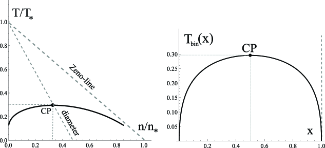
Figure 1: The symmetrization of the vdW binodal using the parametrization (19) corresponding to the linear approximation for the diameter.

The difference between the exact values $n_{c}/n_{*}=1/3,T_{c}/T_{*}=8/27,P_{c}/(n_{*}T_{*})=1/27$ is caused by the deviation of the diameter for the vdW EoS form the linear behavior. As we see the differences are rather  small. Thus simple parametrization (19) can be applied to any EoS where the deviation from the LRD can be neglected. In this case the symmetrization of the binodal described by the parametrization (18) or 19 along with the EoS for the LG could be useful in processing the data of the simulations for the coexistence curve (CC) of the Lennard-Jones fluids, where simple approximate formula:

$$n_{l,g}=n_{c}+A\,|\tau|\pm B_{0}\,|\tau|^{\beta}\,,\quad\tau=\frac{T-T_{c}}{T_{c}}\,,$$ (23)

is used Frenkel and Smit (2001). Also the proposed approach allows to avoid ambiguity in extrapolation of the binodal into the region $T\to 0$ Apfelbaum et al. (2006).

In order to visualize how the splitting of the degenerate elements mentioned above (see p. II) occurs it is expedient to consider the application of the transformation to the classical EoS for the LG the Curie-Weiss molecular field approximation (see e.g. Huang (1987)). This equation of state has the form:

$$h(m,t)=t\,{\rm ArcTanh}\,(m)-m\,,\quad m=2x-1\,.$$ (24)

The isotherms for this model EoS are shown in 2 (a). The linear character of the transformation (9) with respect to the order parameters $x$ and $n$ allows to connect the pressure for the asymmetrical liquid $P_{liq}(T,\mu)$ with that of the LG as follows:

$$P_{liq}(T,\mu)=P_{LG}(t(T),h(\mu,T))\,.$$ (25)

The dependence $h(\mu,T)$ will be obtained in Section IV (see (32) below). The pressure for the LG $P_{LG}$ and in particular for EoS 24 can be defined by the standard method (see e.g. Rice (1967)). Taking into account the conjugation of the thermodynamic variables we can write:

$$P_{LG}(t,h)=f(t,m)+\frac{m+1}{2}\,h\,,$$ (26)

where $f(t,m)$ is the thermodynamic potential for the variables $(t,m)$. It is constructed easily using EoS (24) so that:

$$h(t,m)=\left.\frac{\partial\,f}{\partial\,m}\right|_{t}\,.$$ (27)

Substituting (26) into (25) we are able to construct the isotherms in $n-T$ plane. The result of construction of the isotherms and the binodal of the “fluid“ in coordinates “pressure-density“ basing on the Curie-Weiss EoS (24) for the LG is shown in 2.

In the following Section we discuss the relation between the thermodynamic functions of the LG and its continuum analog in detail.

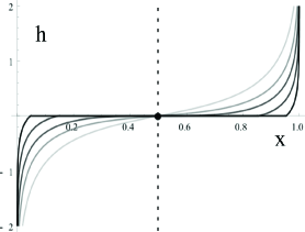
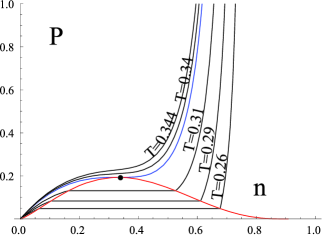
Figure 2: The isotherms obtained using (9) applied to Curie-Weiss approximation for LG with $z=1/2$. The isotherms of (24) are shown in Fig. (a). The corresponding isotherms for the isomorphic “fluid“ model are in Fig. (b). The red curve is the binodal, the critical isotherm $T_{c}=1/3$ is marked by the blue line. The quantities are dimensionless (see (22)).

IV The relation between the thermodynamic potentials of the fluid and the Lattice Gas

Basing on the analysis of Apfelbaum and Vorob’ev (2010); Kulinskii (2010c) one can expect that the transformation (9) gives the relation between phase diagram of the LG and that of the real fluid at least as the “zeroth order approximation“. The idea that the difference between irregularity configuration for continuum fluids and regularity of configurations of lattice models is unimportant for consideration of the order-disorder transitions in the fluctuational region is due to K.S. Pitzer (see Pitzer (1989)). But beyond the fluctuational region the shape of the holes in real or continuum liquid and that in the lattice gas causes the main difference between the configurations of these systems. From this point of view the global character of the transformation 9 shows that the particle-hole simplified picture still can be useful. Though, it is not the particle density which reflects such symmetry. Rather the combination of the density of the particles and the density of the holes is the symmetrical variable (see p. 3). This rehabilitates the hole theory for expanded liquids Rice (1967); Barker and Henderson (1976). Such caricature picture of the liquid state gives the possibility to relate the thermodynamic functions of these systems.

Let

$$\mathfrak{G}(t,h,\mathcal{N})=\mathcal{N}\,\mathfrak{g}(t,h)\,,\quad\text{and}\,\quad J(T,\mu,V)=P(T,\mu)\,V\,,$$

are the thermodynamic potentials of the grand canonical ensembles for the LG and the fluid correspondingly. Here $\mathcal{N}$ is the number of sites in a lattice. First it is natural to state the following relation $\mathcal{N}=n_{*}\,V$ between the extensive variables of these ensembles. The results of  Apfelbaum et al. (2008) allow to interpret $1/n_{*}$ as the volume per particle in the ideal crystal state at $T\to 0$. Such a state defines the lattice which may serve as the basis for the determination of the corresponding Lattice Gas model.

Using the standard definitions:

$$n=\frac{1}{V}\left.\frac{\partial\,J}{\partial\,\mu}\right|_{T}\,,\quad x=\frac{1}{\mathcal{N}}\left.\frac{\partial\,\mathfrak{G}}{\partial\,h}\right|_{t}$$ (28)

along with (9) we get the following relation between the potentials:

$$J(\mu,T,V)=\mathfrak{G}\left(\,h(\mu,T),t(T),\mathcal{N}\,\right)\,\Rightarrow P(\mu,T)=n_{*}\,\mathfrak{g}\left(\,h(\mu,T),t(T)\,\right)\,.$$ (29)

From (9) the relation between the density of the fluid and the density of the LG can be written as following:

$$n(\mu,T)/n_{*}=x(h(\mu,T),t(T))\,\left(\,1-T/T_{*}\,\right)\,.$$ (30)

Taking into account trivial relation:

$$\left.\frac{\partial\,}{\partial\,\mu}\right|_{T}=\left.\frac{\partial\,h}{\partial\,\mu}\right|_{T}\left.\frac{\partial\,}{\partial\,h}\right|_{t}\,,$$

from (28),29 and (30) we get the following relation:

$$h(\mu,T)=\left(\,1-T/T_{*}\,\right)\left(\,\mu-\mu_{0}(T)\,\right)\,,$$ (31)

or, in the inverse form:

$$\mu-\mu_{0}(T)=h\,\left(\,1+z\,t\,\right)\,\,.$$ (32)

We remind that $h=0$ below CP is the coexistence line for the LG and is mapped onto the saturation curve of the continuum fluid. Therefore $\mu_{0}(T)$ coincides with the chemical potential $\mu_{s}(T)$ along the saturation curve below the critical point $T<T_{c}$. To determine $\mu_{0}(T)$ in the supercritical region $T>T_{c}$ we note that the line

$$n(\mu_{0}(T),T)/n_{*}=\frac{1-T/T_{*}}{2}\,,$$ (33)

is the image of the line of symmetry $h=0$ for the LG along which $x=1/2$.

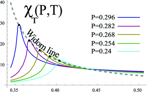
Figure 3: Widom line (dashed) as the line of the temperature maxima of the isothermal compressibility $\chi_{T}(P,T)$ of the fluid for different $P$. It is given by (33). The compressibility is calculated using the Curie-Weiss EoS (24) with subsequent transformation (9).

Therefore $\mu_{0}(T)$ defined by (33) can be considered as the Widom-Stillinger line of symmetry for the liquid Widom and Rowlinson (1970); *crit_diampartholewidom_jcp1973. Indeed, such line is defined as the locus of maximum of correlation length where the thermodynamic response function such as the isothermal compressibility $\chi_{T}=\frac{1}{n}\,\left.\frac{\partial\,n}{\partial\,p}\right|_{T}$ has maxima $T_{max}(P)$ Franzese and Stanley (2007). Obviously, in case of the LG it is represented by the line $h=0$, or equivalently by the critical isochore $x=1/2$.

The Widom-Stillinger line has attracted much attention recently in the studies on supercritical states of liquids Gorelli et al. (2006); Simeoni et al. (2010). The stated mapping between the LG and the fluid naturally explains the separation of the fluid region into the gas-like and the liquid-like states with the Widom line as the border. The gas-like region is the image of the region $x<1/2$ where the number of holes is greater than the number of particles. For the liquid-like region $x>1/2$ the situation is inverse.

The line (33) is the image of the line $h=0$. Therefore along this line the continuation of the subcritical behavior (divergence) of the isothermal compressibility $\chi_{T}$ takes place. Fig. 3 shows the result of the calculations for the compressibility $\chi_{T}$ in accordance with the relation 29 between the fluid and the LG. This is the locus of the compressibility maxima.

From (29) the relation between the entropy $\mathfrak{S}$ of the LG and that of the fluid $S$ can be derived:

$$S(T,\mu,V)=\left.\frac{\partial\,J}{\partial\,T}\right|_{\mu}=\frac{d\,t}{d\,T}\left.\frac{\partial\,\mathfrak{G}}{\partial\,t}\right|_{h}=\frac{\left(\,1+z\,t\,\right)^{2}}{z}\,\mathfrak{S}(t,h,\mathcal{N})\,.$$ (34)

The results described above illustrate the general analysis of Rehr and Mermin (1973). The mapping 9 determines the fluid as the asymmetric model for the symmetric LG. The conservation of the RDL is due to the direct relation between the the thermodynamic potentials 29. Indeed, if linear relation between $P(\mu,T)$ and $\mathfrak{g}(h(\mu,T),t(\mu,T))$ with the analytic coefficients holds, then the quantity $\left.\frac{\partial\,P(\mu,T)}{\partial\,h}\right|_{T}$ has the rectilinear diameter. This order parameter is the combination of the density and the entropy Rehr and Mermin (1973); Wang and Anisimov (2007).

In order to be physically meaningful, the transformation 9 or its generalization should appear as the average of the transformation of the microscopic variables. We assume that there exist such transformation which leads to the symmetrization of the binodal. The similarity between the liquid-vapor part of the diagram for the fluid and that of the LG and also the separation between the liquid-like and gas -like states (see e.g. Simeoni et al. (2010)) allows to state that for the case of fluids there exists the “asymmetrical“ microscopic observable $\mathcal{A}$ such that:

$$\left\langle\,\mathcal{A}\,\right\rangle_{l}+\left\langle\,\mathcal{A}\,\right\rangle_{g}=0\,.$$ (35)

Here $\left\langle\,\ldots\,\right\rangle_{l,g}$ stands for the averages on the corresponding coexisting liquid and gaseous states with $(T,n_{l}(T))$ and $(T,n_{g}(T))$. In terms of Griffiths and Wheeler (1970) the equilibrium average $\left\langle\,\mathcal{A}\,\right\rangle_{l,g}\neq 0$ is the density-like variable, which takes different values in the coexisting phases. The specific form of the observable depends on the Hamiltonian of the fluid. Such observable exists in case of penetrable sphere models where the relation between the thermodynamic potentials $P$ and $\mathfrak{g}$ is linear Rehr and Mermin (1973). In fact the right hand side in 35 can be any analytic function of $T$ (including the neighborhood of the CP). In such case it is possible to redefine $\mathcal{A}$ so that (35) is fulfilled. Then the following equation

$$\left\langle\,\mathcal{A}\,\right\rangle_{\mu,T}=0\,\,,$$ (36)

determines the continuation $\mu_{0}(T)$ of the diameter into the supercritical region $T>T_{c}$. Once such observable is determined the corresponding thermodynamic potential can be defined so that

$$\left\langle\,\mathcal{A}\,\right\rangle=\left.\frac{\partial\,\mathfrak{F}}{\partial\,h_{\mathcal{A}}}\right|_{S}\,\,.$$

In general $\mathfrak{F}$ depends on the field variables $P,\mu,T$ nonlinearly. Therefore, in accordance with Griffiths and Wheeler (1970); Rehr and Mermin (1973) the density diameter shows both $1-\alpha$ and $2\beta$ anomalies. Since the singularity of the diameter is of fluctuational nature the transformation (9) should be considered as the mean-field approximation for the transformation between microscopic fields (see Kulinskii and Malomuzh (2009)).

V The cubic shape of the binodal

The fact of the global cubic shape of the CC for the molecular liquids is the long standing issue and was well known to van der Waals due to studies of Verschaffelt Verschaffelt (1896) (see also the review Sengers (1975)). It is also well established fact for a wide variety of the Lennard-Jones fluids with the short ranged interactions. The results of computer simulations are well described by the Guggenheim-like expression 23 (see Guggenheim (1945)).

The transformation (9) states that the shape of the CC for the molecular fluids is determined by that for the LG Kulinskii (2010b). As is known from the computer simulations Luijten and Binder (1998) the crossover to the classical behavior which is characterized by the parabolic shape of the binodal is absent for the LG with the nearest neighbors interaction. On the basis of the global character of the transformation (9) one can assume that the same is true for the molecular fluids with the short-ranged potentials. In other words, the binodal of the molecular fluid can be described approximately by the global cubic dependence similar to (23) in a broad temperature interval. In Kulinskii (2010c) this statement was demonstrated for 2D and 3D Lennard-Jones fluids. In particular the binodal of the 2D Lennard-Jones fluid was obtained as the image of the binodal of the 2D Ising model given by the Onsager exact solution. In such a case very flat shape of the binodal dome of 2D fluid is due to the exponent $\beta=1/8$ and the global nature of the power-like dependence of the binodal of the 2D LG:

$$x=1/2\pm f(t)^{1/8}\,,\quad f(t)=1-\frac{1}{{\rm Sinh}(2J/t)}\,.$$

Note that $f(t)$ is the analytic function of the LG temperature variable $t$.

The classical Landau theory of the phase transitions gives the general picture which is characterized by the classical exponents for the critical asymptotics of the thermodynamic quantities Landau and Lifshitz (1980). In particular the dome of the binodal is given by the the quadratic curve. But it should be stressed that the Landau theory breaks the continual character of change of the thermodynamic state in passing through the CP. Indeed, there is the discontinuity of the specific heat $C_{V}$ and therefore there is no unique critical state but still there are two coexisting phases.

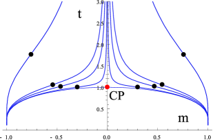
(a)   LG

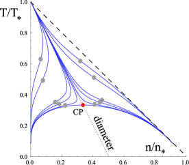
(b)   liquid

Figure 4: The phase diagram of the LG (the Ising model) and its mapping to $(n,T)$ plane of liquid states with the help of (9). The points mark the positions of the inflection points (see the text). The red point is the CP. Two families with $h>0$ and $h<0$ of iso-h lines $t(h,m)$ (a) and their images in $n-T$ plane (b) are shown. The binodal is the limiting curve of these families.

This discontinuity is connected with the assumption of the existence of the only strongly fluctuating quantity. For the liquid-vapor critical point such quantity is the density. Indeed, if the entropy is used as the order parameter then the finite jump of the specific heat allows to distinguish between the ordered and the disordered phase at the CP. Besides, the parabolic shape of the binodal is the consequence of the usage of analytic EoS with applying the Maxwell construction for the pair of conjugated variables (e.g. the pressure and the volume) in the subcritical region. This puts the constraint of analyticity of the binodal in terms of other pair of the variables, e.g. the temperature and the entropy. Note that in the vicinity of the critical point $t(\tilde{x})$ should be the even function of the order parameter (see (17)). One can expect that weak divergence of the specific heat admits the analyticity of the function $t(\tilde{x})$. Then $t(\tilde{x})=1-b_{0}\,\tilde{x}^{2n}+\ldots\,,b_{0}>0$, where $n>0$ is the integer. Obviously, this occurs in $d=2$ and $d\geq 4$, where the specific heat has weak logarithmic divergence or finite jump with $n=4$ and $n=1$ correspondingly. For $d=3$ the specific heat diverges more strongly. Therefore one could expect that the analyticity of $t(\tilde{x})$ breaks in this case.

To clarify where the possibility for the global cubic shape of the binodal appears let us consider the $t-m$ phase diagram of the LG (Ising model). We use the Ising-like order parameter $m=2x-1$ for the convenience and consider the family of the iso-$h$ curves $t(h,m)$ for the LG. Notably, all these curves has the inflection points $m_{0}(h)$. Fig. 4 shows the situation for the Curie-Weiss EoS (24). Obviously, in the vicinity of the inflection point $m_{0}(h)$ determined by the condition:

$$\left.\frac{\partial^{2}\,t(h,m)}{\partial\,m^{2}}\right|_{m=m_{0}}=0\,,$$

the function $t(h,m)$ has the cubic form (see 4):

$$t(h,m)=t_{0}(h)+t_{1}(h)\,\left(\,m-m_{0}(h)\,\right)+\frac{t_{3}(h)}{6}\,\left(\,m-m_{0}(h)\,\right)^{3}+\ldots\,\,,$$ (37)

where the coefficients $t_{1}(h)$ and $t_{3}(h)$ are the odd functions of $h$. Naturally, the binodal as the line of the phase equilibrium is the curve which correspond to $h=0$. From this point of view the binodal consists of two parts. They are the limiting curves of the families of cubics (37) with $h>0$ and $h<0$ correspondingly (see Fig. 4). Therefore the binodal as the limiting curve for these families should have the cubic form:

$$t(0\pm 0,m)=1-\frac{t^{(0)}_{3}}{6}\,m^{2}\,|m|+\ldots\,\,.$$ (38)

or, equivalently

$$m=B_{0}|\tau|^{1/3}+\ldots\,,$$ (39)

where

$$B_{0}=\left(\,\frac{6}{t^{(0)}_{3}}\,\right)^{1/3}\,.$$ (40)

In the mean-field approximation $t_{3}(h)\to\infty$ in the CP. But the analysis of the simplest Curie-Weiss approximation shows that it is reasonable to use the extrapolated value $t^{(0)}_{3}$ (see Fig. 5).

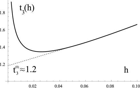
Figure 5: The behavior of the coefficient $b(h)$ in the Curie-Weiss approximation. The extrapolation is shown by the dashed line.

From (40) we obtain the value of the amplitude for the binodal opening $B_{0}\approx 1.7$. Surprisingly, this coincides with the result of the corresponding value obtained in the computer simulations for the 3D Ising model Talapov and Blote (1996). Under the transformation 9 the iso-$h$ lines map onto the corresponding ones in $n-T$ plane (see Fig. 4). Obviously, the local cubic character similar to (37) near the inflection points takes place. Approaching the CP we obtain the relation between the amplitudes of the LG and the continuum fluid:

$$B^{(f)}_{0}=(1+z)^{1/3}\,B_{0}\,.$$ (41)

In accordance with the results Kulinskii (2010b) for the Lennard-Jones fluids, where the attractive part of the interaction has the “$-1/r^{6}$“ behavior, $z=1/2$ in $d=3$. Then, from (40) and (41) we get:

$$B^{(LJ)}_{0}\approx 1.95\,,$$ (42)

which is good agreement with the value obtained in computer simulations $B_{0}\approx 1.92\div 2.0$ for potentials of “$6-n$“ type Okumura and Yonezawa (2000); *crit_longrangecampatey_jcp2001; *eos_ljfluid_jcp2005.

This allows to treat the value $\beta=1/3$ as the corresponding exponent which conforms with the continuity of the critical state for $d=3$ for the systems isomorphic to the LG. Other critical indices, except the small ones $\alpha$ and $\eta$ which in the mean-field approximation are zeroth, can be obtained via the standard thermodynamic stability and scaling reasonings, so that $\nu=2/3,\,\gamma=4/3,\,\delta=5$ etc.

VI Conclusions

In this paper the explicit relations between the basic thermodynamic functions of the LG and the continuum fluid is derived within the global isomorphism approach proposed in Kulinskii (2010a). These relations allow to obtain the information about liquid state directly from the EoS for the lattice model. It is quite remarkable since the lattice models do not contain the translational degrees of freedom. Nevertheless, as it follows from the results Kulinskii (2010c); Apfelbaum and Vorob’ev (2010) this mapping gives rather good description for the LJ fluids. In particular the stated relations can be used to connect the computer simulations for the lattice models with those for the continuum fluids (see  Kulinskii (2010c)). Within such an approach the splitting between critical isochore and the diameter, the Zeno-line and the tangent to the binodal at $T\to 0$ is naturally described. The conservation of linear character of the diameter allows to obtain simple form of the transformation between the phase diagram of the LG and the continuum fluid. Obviously, the value of the critical density is the most sensitive to such approximation. But for the computer simulations the deviations from the law of rectilinear diameters are small to observe them near the CP Frenkel and Smit (2001). This explains rather good agreement of the estimates for the locus of the CP based on the parametrization (9) for the Lennard-Jones fluids with the results of the computer simulations Bulavin and Kulinskii (2010).

We believe that the approach proposed could be useful in studies of the supercritical behavior basing on the EoS of the lattice models especially for water Franzese and Stanley (2007); Abascal and Vega (2010) where a lot of lattice models, including the models with H-bond are known. In view of the results of work Simeoni et al. (2010) it would be interesting to generalize the proposed approach in order to search the correspondence between the dynamic response functions of fluids and their lattice analogues. This poses the question about the choice of the adequate lattice model of the proper geometry and the type of the interaction which realizes the isomorphism with the corresponding fluid.

References

- Cailletet and Mathias (1886) L. Cailletet and E. Mathias, Comptes rendus hebdomadaires des séances de l’Académie des Sciences 102, 1202 (1886).
- Young (1900) S. Young, Proceedings of the Physical Society of London 17, 480 (1900).
- Tsuruta. (1900) K. Tsuruta., Phys. Rev. (Series I) 10, 116 (1900).
- Guggenheim (1945) E. A. Guggenheim, The Journal of Chemical Physics 13, 253 (1945).
- Batschinski (1906) A. Batschinski, Ann. Phys. 324, 307 (1906).
- Hansen and Mcdonald (2006) J.-P. Hansen and I. R. Mcdonald, Theory of Simple Liquids, Third Edition (Academic Press, 2006).
- Landau and Lifshitz (1980) L. D. Landau and E. M. Lifshitz, Statistical Physics (Part 1), 3rd ed. (Pergamon Press, Oxford, 1980).
- Ben-Amotz and Herschbach (1990) D. Ben-Amotz and D. R. Herschbach, Israel Journal of Chemistry 30, 59 (1990).
- Xu and Herschbach (1992) J. Xu and D. R. Herschbach, The Journal of Physical Chemistry 96, 2307 (1992).
- Song and Mason (1992) Y. Song and E. A. Mason, Journal of Physical Chemistry 96, 6852 (1992).
- Apfelbaum et al. (2004) E. M. Apfelbaum, V. S. Vorob’ev, and G. A. Martynov, Journal of Physical Chemistry A 108, 10381 (2004).
- Apfelbaum et al. (2006) E. M. Apfelbaum, V. S. Vorob’ev, and G. A. Martynov, Journal of Physical Chemistry B 110, 8474 (2006).
- Apfelbaum and Vorob’ev (2009) E. M. Apfelbaum and V. S. Vorob’ev, The Journal of Chemical Physics 130, 214111 (2009).
- Patashinskii and Pokrovsky (1979) A. Z. Patashinskii and V. L. Pokrovsky, Fluctuation theory of critical phenomena (Pergamon, Oxford, 1979).
- Rehr and Mermin (1973) J. J. Rehr and N. D. Mermin, Physical Review A 8, 472 (1973).
- Kim et al. (2003) Y. C. Kim, M. E. Fisher, and G. Orkoulas, Physical Review E: Statistical, Nonlinear, and Soft Matter Physics 67, 061506 (2003).
- Wang and Anisimov (2007) J. Wang and M. A. Anisimov, Physical Review E (Statistical, Nonlinear, and Soft Matter Physics) 75, 051107 (2007).
- Kulinskii and Malomuzh (2009) V. Kulinskii and N. Malomuzh, Physica A: Statistical Mechanics and its Applications 388, 621 (2009).
- Reagan and Tester (2001) M. T. Reagan and J. W. Tester, Int. J. Thermophys. 22, 149 (2001).
- Kulinskii (2010a) V. L. Kulinskii, Journal of Physical Chemistry B 114, 2852 (2010a).
- Bulavin and Kulinskii (2010) L. A. Bulavin and V. L. Kulinskii, The Journal of Chemical Physics 133, 134101 (2010).
- Kulinskii (2010b) V. L. Kulinskii, The Journal of Chemical Physics 133, 034121 (2010b).
- Kulinskii (2010c) V. L. Kulinskii, The Journal of Chemical Physics 133, 131102 (2010c).
- Sengers (1970) J. M. L. Sengers, Ind. Eng. Chem. Fundam. 9, 470 (1970).
- Apfelbaum and Vorob’ev (2008) E. M. Apfelbaum and V. S. Vorob’ev, J. Phys. Chem B. 112, 13064 (2008).
- Rah and Eu (2001) K. Rah and B. C. Eu, The Journal of Chemical Physics 115, 2634+ (2001).
- Rah and Eu (2003) K. Rah and B. C. Eu, Journal of Physical Chemistry B 107, 4382 (2003).
- Apfelbaum and Vorob’ev (2010) E. M. Apfelbaum and V. S. Vorob’ev, The Journal of Physical Chemistry B 114, 9820 (2010).
- Ma (1976) S. Ma, Modern theory of critical phenomena (W.A. Benlamin, Inc., London, 1976).
- Frenkel and Smit (2001) D. Frenkel and B. Smit, Understanding Molecular Simulation, Second Edition: From Algorithms to Applications (Computational Science Series, Vol 1), 2nd ed. (Academic Press, 2001).
- Huang (1987) K. Huang, Statistical Mechanics, 2nd Edition, 2nd ed. (Wiley, 1987).
- Rice (1967) O. Rice, Statistical Mechanics, Thermodynamic and Kinetics (W.H. Freeman and Co, 1967).
- Pitzer (1989) K. S. Pitzer, Pure and Applied Chemistry 61, 979 (1989).
- Barker and Henderson (1976) J. A. Barker and D. Henderson, Rev. Mod. Phys. 48, 587 (1976).
- Apfelbaum et al. (2008) E. M. Apfelbaum, V. S. Vorob’ev, and G. A. Martynov, Journal of Physical Chemistry A 112, 6042 (2008).
- Widom and Rowlinson (1970) B. Widom and J. S. Rowlinson, The Journal of Chemical Physics 52, 1670 (1970).
- Widom and Stillinger (1973) B. Widom and F. H. Stillinger, The Journal of Chemical Physics 58, 616 (1973).
- Franzese and Stanley (2007) G. Franzese and H. E. Stanley, J. Phys.: Condens. Matter 19, 205126+ (2007).
- Gorelli et al. (2006) F. Gorelli, M. Santoro, T. Scopigno, M. Krisch, and G. Ruocco, Phys. Rev. Lett. 97, 245702 (2006).
- Simeoni et al. (2010) G. G. Simeoni, T. Bryk, F. A. Gorelli, M. Krisch, G. Ruocco, M. Santoro, and T. Scopigno, Nat Phys 6, 503 (2010).
- Griffiths and Wheeler (1970) R. B. Griffiths and J. C. Wheeler, Phys. Rev. A 2, 1047 (1970).
- Verschaffelt (1896) J. E. Verschaffelt, Conmun. Phys. Lab., Leiden 2, 1 (1896).
- Sengers (1975) J. M. H. W. Sengers, Physica A: Statistical Mechanics and its Applications 82, 319 (1975).
- Luijten and Binder (1998) E. Luijten and K. Binder, Physical Review E: Statistical, Nonlinear, and Soft Matter Physics 58, R4060 (1998).
- Talapov and Blote (1996) A. L. Talapov and H. W. J. Blote, Journal of Physics A: Mathematical and General 29, 5727 (1996).
- Okumura and Yonezawa (2000) H. Okumura and F. Yonezawa, The Journal of Chemical Physics 113, 9162 (2000).
- Camp and Patey (2001) P. J. Camp and G. N. Patey, The Journal of Chemical Physics 114, 399 (2001).
- Ou-Yang et al. (2005) W.-Z. Ou-Yang, Z.-Y. Lu, T.-F. Shi, Z.-Y. Sun, and L.-J. An, The Journal of Chemical Physics 123, 234502 (2005).
- Abascal and Vega (2010) J. L. F. Abascal and C. Vega, The Journal of Chemical Physics 133, 234502 (2010).