On free stochastic differential equations

Abstract

The paper derives an equation for the Cauchy transform of the solution of a free stochastic differential equation (SDE). This new equation is used to solve several particular examples of free SDEs.

1. Introduction

Free stochastic differential equations generalize classical stochastic differential equations to the setting of free probability. Here is an example of such an equation:

$$X_{t}=a(X_{t})dt+b^{\ast}(X_{t})(dZ_{t})b(X_{t})$$

In this equation, $X_{t}$ is a self-adjoint operator, $a(X_{t})$ and $b(X_{t})$ are operator-valued functions of $X_{t}$, and the driving noise $Z_{t}$ is an operator process with free increments. That is, the increments $Z_{s}-Z_{t},$ $s>t,$ are assumed to be free from past realizations of $Z_{t}.$ The process $Z_{t}$ is usually the free Brownian process, in which case the increments have semicircle distributions; however, other choices are possible.

Informally, the reader may think about $X_{t}$ as very large random matrices and $Z_{t}$ as matrices with independent Gaussian random variables as entries. These entries follow independent Brownian motions and we are interested in the law of the eigenvalues of $X_{t}.$ The free probability theory is a convenient abstraction which intends to model the situation when the size of the matrices is very large.

The study of free stochastic differential equations (“free stochastic calculus”) is more difficult than in the classical case because of non-commutativity of coefficients and noise. This paper contributes by developing a new tool for the analysis of these equations.

The idea of free stochastic calculus was first suggested in [S]. It was later developed and formalized in [KS], [B], [BSa], and [A], which introduced stochastic integration with respect to free Brownian motion as a rigorous basis for free stochastic calculus. They also derived an analog of the Itô formula, which allows us to obtain identities like the following:

$$\int_{0}^{a}[W_{t}^{2}(dW_{t})+W_{t}(dW_{t})W_{t}+(dW_{t})W_{t}^{2}]=W_{a}^{3}-2\int_{0}^{a}W_{t}dt,$$

where $W_{t}$ denotes the free Brownian motion (the Wigner process).  An analogous formula in the classical situation is

$$\int_{0}^{a}3B_{t}^{2}(dB_{t})=B_{a}^{3}-3\int_{0}^{a}B_{t}dt,$$

where $B_{t}$ is the standard Brownian motion. Note the different coefficient before the integral on the right-hand side.

The classical Itô formula is very helpful in the study of stochastic differential equations. Unfortunately, the range of applicability of the free Itô formula is smaller. This difficulty calls for a different method applicable to those free SDEs, which are not solvable with the Itô formula. One possibility is to seek an equation for the evolution of the spectral distribution of the solution. Such an equation was derived by Biane and Speicher in [BSb] for the equation

$$X_{t}=a(X_{t})dt+dW_{t}.$$ (1)

They showed that the density of the spectral probability measure of $X_{t},$ which we denote $p_{t}$ and which generalizes the eigenvalue distribution of a matrix, satisfies the free Fokker-Planck equation:

$$\frac{\partial p_{t}}{\partial t}=-\frac{\partial}{\partial x}[p_{t}(Hp_{t}+a)].$$ (2)

Here $H$ denotes a multiple of the Hilbert transform:

$$Hu(x):=\mathrm{p.v.}\int\frac{u(y)}{x-y}dy.$$ (3)

Still, the approach through the free Fokker-Planck equation has its own disadvantages. First, it is applicable only to equations that have the special form (1), that is, only to equations with the constant diffusion coefficient. Second, the free Fokker-Planck equation (2) is not a bona fide partial differential equation since it includes the Hilbert transform operator. For this reason, it is somewhat difficult to solve this equation.

The purpose of this paper is to approach the free stochastic equations by deriving a differential equation for the Cauchy transform of the solution.

Recall that the resolvent of operator $X_{t}$ is defined as the operator-valued function of a complex parameter $G_{t}\left(z\right):=\left(X_{t}-z\right)^{-1}.$ The Cauchy transform of $X_{t}$ is defined as the expectation of the resolvent: $g_{t}(z):=E[\left(X_{t}-z\right)^{-1}].$ It is useful because the knowledge of the Cauchy transform is sufficient to recover all  properties of the spectral probability distribution of $X_{t}$. It turns out that if $X_{t}$ solves

$$dX_{t}=a(X_{t})dt+b(X_{t})(dW_{t})c(X_{t}),$$

then $g_{t}(z)$ satisfies the following equation:

$$\frac{dg_{t}}{dt}=-E(a_{t}G_{t}^{2})+E(b_{t}c_{t}G_{t})E(b_{t}c_{t}G_{t}^{2}),$$ (4)

where we use $a_{t},$ $b_{t},$ and $c_{t}$ to denote $a(X_{t}),$ $b(X_{t}),$ and $c(X_{t}),$ respectively. This is the statement of Theorem 3.2 below.

Equation (4) is not a usual differential equation since it involves expectations. In general, these expectations are difficult to compute because the coefficients $a_{t},$ $b_{t},$ and $c_{t},$ and the resolvent $G_{t}$ are not free from each other. However, if the coefficients are polynomials, it is possible to perform further reduction to a differential equation as we will show in Proposition 3.4.

As we just said, the knowledge of the Cauchy transform can be used to recover the spectral probability distribution. In particular, the free Fokker-Planck equation (2) can be derived from (4) as will be shown in Corollary 3.6.

In certain cases it is not possible to compute the Cauchy transform explicitly, but it is possible to detect the behavior of its singularities. This knowledge can provide us with information about the support of the spectral distribution. In particular, it can show us how the norm of the solution grows.

For a simple example of this approach, let us consider the well-known case of the free Ornstein-Uhlenbeck equation:

$$dX_{t}=-\theta X_{t}dt+\sigma dW_{t}.$$ (5)

For this equation, it is easy to compute the Cauchy transform using equation (4) and recover the known result that for positive $\theta,$ the spectral probability distribution of $X_{t}$ converges to a stationary solution, which is a semicircle distribution supported on the interval $[-\sigma\sqrt{2/|\theta|},\sigma\sqrt{2/|\theta|}].$

As a more difficult example, consider the equation

$$dX_{t}=\theta X_{t}dt+X_{t}^{1/2}(dW_{t})X_{t}^{1/2},$$

which can be thought of as a free analog of the equation for the “geometric Brownian motion”, $dx_{t}=\theta x_{t}dt+x_{t}dB_{t}.$

Let $X_{0}=I.$ Equation (4) leads to the following differential equation:

$$\frac{\partial g}{\partial t}+z(\theta-1-zg)\frac{\partial g}{\partial z}=-g(\theta-1-zg),$$

with the initial condition $g\left(0,z\right)=\left(1-z\right)^{-1}.$ The method of characteristics gives us a functional equation for the Cauchy transform:

$$z+g^{-1}=e^{(\theta-1-zg)t}.$$ (6)

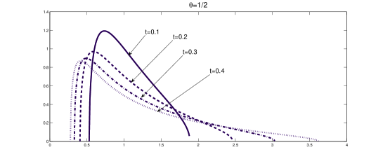
Figure 1. $\theta=1/2$

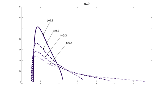
Figure 2. $\theta=2$

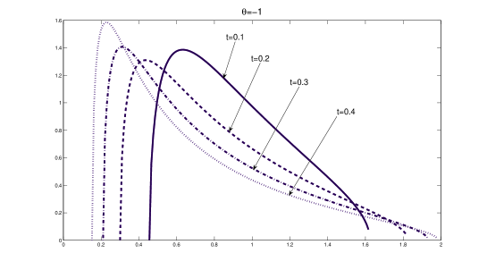
Figure 3. $\theta=-1$

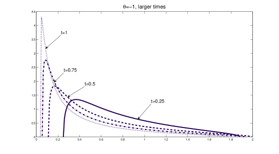
Figure 4. $\theta=-1,$ Large times

While it is difficult to extract an explicit analytical formula for the solution of this equation, we can investigate how the support of the distribution changes with time. It turns out that for $\theta<0,$ the support of the distribution shrinks to zero. If $\theta$ is between $0$ and $1,$ then the lower boundary of the support decreases to zero and the upper boundary grows exponentially fast to infinity. If $\theta>1,$ then both the lower and upper boundary of the support grow exponentially fast to infinity.

We can solve equation (6) numerically and recover the density of the spectral distribution by using Stieltjes formula. Figures 1-4 show the evolution of the density for various values of parameters and illustrate the complexity of the behavior of the spectral distribution. For example, Figure 2 shows that even if $\theta>1,$ the spectral distribution does not approach infinity immediately. There is a transition period in which a significant portion of the spectral distribution remains below $\lambda=1.$ Similarly, Figure 3 shows that for $\theta<0,$ the distribution does not collapse to zero immediately. Only when time increases, the distribution begins the rapid approach to zero, as shown in Figure 4.

Let us compare this result with the classical analog. By using the Itô formula, it is easy to show that the solution of the classical equation for the geometric Brownian motion is

$$x_{t}=\exp\{(\theta-\frac{1}{2})t+B_{t}\}.$$

Hence, with probability $1,$ the classical solution will decrease exponentially to zero if $\theta<1/2,$ and will grow exponentially to infinity if $\theta>1/2.$ However, the support of the solution distribution is $(0,\infty)$ for all $t$. This is quite unlike the behavior of the free SDE solution.

Note that the equation for the geometric Brownian motion can be generalized to the free probability setting in a different way:

$$dX_{t}=\theta X_{t}dt+X_{t}dW_{t}+(dW_{t})X_{t}.$$

The behavior of the solution of this equations is quite different. In particular, the ratio of the standard deviation to the expectation is $\sqrt{2(e^{2t}-1)}.$ This ratio grows exponentially fast with $t,$ quite unlike the previous example, where this ratio equals $\sqrt{t}.$ Unfortunately, the partial differential equation associated with equation is more difficult to solve and it is not clear whether the solution becomes unbounded in finite time.

Finally, let us consider the following equation:

$$dX_{t}=kX_{t}(dW_{t})X_{t},$$

and let the initial condition be $X_{0}=aI.$ For this equation it is possible to write an explicit formula for the spectral distribution of the solution. An interesting feature of this equation is that the solution blows up in finite time $\tau=(ak)^{-2},$ by which we means that the operator norm of the solution becomes infinite as $t$ approaches $\tau$.

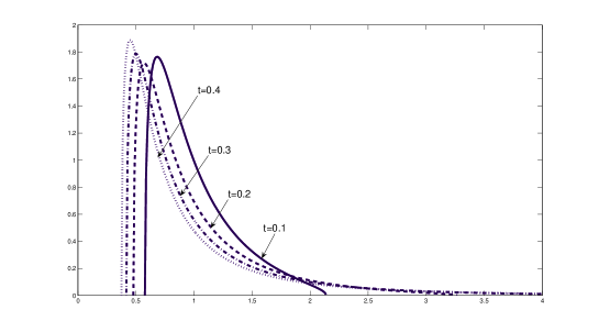
Figure 5. Density functions for $t=0.1$, $0.2$, $0.3$, $0.4$.

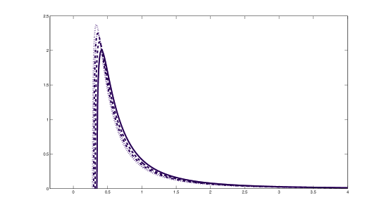
Figure 6. Density functions for $t=0.5$, $0.6$, $0.7$, $0.8$

Another interesting feature is that as time $t$ approaches $\tau,$ the spectral distribution converges to a fixed distribution. If $k=a^{-1}$, then the density of this distribution is

$$f\left(\xi\right)=\frac{\sqrt{4\xi-1}}{2\pi\xi^{3}},$$

which is supported on the interval $\left[1/4,\infty\right).$ Otherwise, it is a scaled version of this distribution. The behavior of the solution density for various times is illustrated in Figures 5 and 6.

Several specific classes of free SDE have already been investigated in the literature. Biane and Speicher in [BSb] and Gao in [G] studied the free Ornstein-Uhlenbeck equation (5). Biane and Speicher proved that its solution converges to a stationary process with a semicircle distribution. Gao considered free Ornstein-Uhlenbeck processes with a free Levy driving noise, and showed that every self-decomposable probability measure on the real line can be realized as a distribution of such a process.

Capitaine and Donati-Matin in [CD-M] defined the free Wishart process and found that it satisfies the free SDE of the form:

$$dX_{t}=\lambda dt+\sqrt{X_{t}}dZ_{t}+dZ_{t}^{\ast}\sqrt{X_{t}},$$

where $Z_{t}$ is the complex Wigner process. Demni in [D] studied the so-called free Jacobi processes which satisfy equations similar to the following:

$$dX_{t}=(\theta I-X)dt+\sqrt{I-X_{t}}dZ_{t}\sqrt{X_{t}}+\sqrt{X_{t}}dZ_{t}^{\ast}\sqrt{I-X_{t}}.$$

With exception of the free Ornstein-Uhlenbeck process, we study a different set of free SDEs, and we approach these equations with a different point of view based on the differential equations for the Cauchy transform.

For the free Ornstein-Uhlebeck process, our results agree with results in [BSb].

The rest of the paper is organized as follows. Section 2 provides preliminary information about free stochastic integration and Itô formulas. Section 3 describes main results. . In particular, Section 3.1 is devoted to a local existence and uniqueness result. Section 3.2 presents general results about the Cauchy transform of the solution and Section 3.3 provides examples.

2. Free Stochastic Integration

2.1. The free Brownian motion

For the basics of free probability theory we refer to [VDN] and [NS]. All operators that we consider belong to a non-commutative $W^{\ast}$-probability space $(\mathcal{A},E)$, that is, to a von Neumann operator algebra $\mathcal{A}$ with a faithful normal trace $E$. We denote the usual operator norm by $\|X\|$, and the $L^{2}$-norm by $\|X\|_{2}:=\sqrt{E(X^{\ast}X)}$.

The spectral probability distribution of a self-adjoint operator $X\in\mathcal{A}$ is a probability measure $\mu$ on $\mathbb{R}$ such that

$$E\left(X^{k}\right)=\int_{\mathbb{R}}x^{k}\mu\left(dx\right).$$

Its Cauchy transform is the function

$$g_{X}\left(z\right)=\int_{\mathbb{R}}\frac{\mu\left(dx\right)}{x-z}.$$

It can be defined directly in terms of operator $X$ as the expectation of the resolvent: $g_{X}\left(z\right)=E[G_{X}\left(z\right)],$ where $G_{X}\left(z\right):=\left(X-z\right)^{-1}.$ The probability measure $\mu$ can be recovered from its Cauchy transform by the Stieltjes inversion formula:

$$\mu\left(B\right)=\frac{1}{\pi}\lim_{\varepsilon\downarrow 0}\int_{B}\mathrm{Im}g\left(x+i\varepsilon\right)dx,$$ (7)

provided that $B$ is Borel and $\mu\left(\partial B\right)=0.$

This fact is the starting point of our approach, since we will study the evolution of the Cauchy transform as a tool to investigate the evolution of the corresponding probability measure.

The most important concept in free probability theory is that of free independence. Let $\overline{A}_{i}$ denote an arbitrary element of algebra $\mathcal{A}_{i}.$ The sub-algebras $\mathcal{A}_{1},\ldots,\mathcal{A}_{n}$ of algebra $\mathcal{A}$ (and operators that generate them) are said to be freely independent or free, if the following condition holds:

$$E(\overline{A}_{i(1)}\ldots\overline{A}_{i(m)})=0,$$

provided that $E(\overline{A}_{i(s)})=0$ and $i(s+1)\neq i(s)$ for every $s$. Two particular consequences of this definition is that (i) $E(AB)=E(A)E(B)$ if $A$ and $B$ are free, and (ii)

$$E(AX_{1}AX_{2})=E(A^{2})E(X_{1})E(X_{2}),$$ (8)

if $A$ is free from $X_{1}$ and $X_{2}$ and $E(A)=0.$

The free Brownian motion, or the Wigner process, is a family of operators $W_{t},$ where $t\geq 0,$ that satisfies the following properties: (1) $W_{0}=0$; (2) the increments of $W_{t}$ are free in the sense of Voiculescu, i.e., if $t>s,$ then $W_{t}-W_{s}$ is free from the subalgebra $\mathcal{W}_{s}$ which is generated by all $W_{\tau}$ with $\tau\leq s$ , and (3) the spectral distribution of $W_{t}-W_{s}$ is semicircle with zero expectation and variance $t-s.$

The choice of $W_{t}$ is not unique, and in the rest of the paper we assume that a particular realization of $W_{t}$ is fixed.

2.2. Free stochastic integral

Itô-style free stochastic integration with respect to the free Brownian motion was defined and studied in [KS] and [BSa]. Their results show that under certain assumptions on the operator coefficients $a_{t}$ and $b_{t},$ it is possible to define the integral

$$I=\int_{0}^{1}a_{t}(dW_{t})b_{t},$$

where $W_{t}$ is the free Brownian motion.

Let us briefly recall the construction of the integral. For details of the construction, the reader is advised to see Definition 2.2.1 and Section 3 in [BSa] and Section 3 and Theorem 14 in [A]. Suppose that $a_{t}$ and $b_{t}$ are functions of $W_{\tau},$ $\tau\leq t.$ That is, let $a_{t}$ and $b_{t}$ belong to the sub-algebra $\mathcal{W}_{t}$. Assume also that $\max\{\left\|a_{t}\right\|,\left\|b_{t}\right\|\}\leq C$ for all $t\in\left[0,1\right]$ and that $t\rightarrow a_{t}$ and $t\rightarrow b_{t}$ are continuous mappings in the operator norm. Let $t_{0},\ldots,t_{n}$ and $\tau_{1},\ldots,\tau_{n}$ be real numbers such that

$$0=t_{0}\leq t_{1}\leq\ldots\leq t_{n}=1,$$

and

$$0\leq\tau_{k}\leq t_{k-1}.$$

We denote the set of $t_{0},\ldots,t_{n}$ and $\tau_{1},\ldots,\tau_{n}$ as $\Delta$. Let

$$d(\Delta)=\max_{1\leq k\leq n}(t_{k}-\tau_{k}).$$

Consider the sum

$$I(\Delta)=\sum_{i=1}^{n}a_{\tau_{i}}(W_{t_{i}}-W_{t_{i-1}})b_{\tau_{i}}$$

It turns out that as $d(\Delta)\rightarrow 0,$ the sums $I(\Delta)$ converge in operator norm and the limit does not depend on the choice of $t_{i}$ and $\tau_{i}.$ The limit is called the free stochastic integral and denoted as $\int_{0}^{1}a_{t}(dW_{t})b_{t}.$ An important point in the proof of convergence is that the convergence of sums in the operator norm depends on a free analogue of the Burkholder-Gundy martingale inequalities.

A very useful tool in the study of stochastic integrals is the Itô formula. A free probability analogue of the Itô formula was developed in [BSa]. In terms of formal rules, it can be written as follows:

$$a_{t}dt\cdot b_{t}dt = a_{t}dt\cdot b_{t}dW_{t}c_{t}=a_{t}dW_{t}b_{t}\cdot c_{t}dt=0,$$

$$a_{t}dW_{t}b_{t}\cdot c_{t}dW_{t}d_{t} = E(b_{t}c_{t})a_{t}d_{t}dt.$$ (9)

Note that the rule in the second line is significantly different from the classical case. In terms of free stochastic integrals, the second rule can be written as follows:

$$\int_{0}^{1}a_{t}dW_{t}b_{t}\cdot\int_{0}^{1}c_{t}dW_{t}d_{t} = \int_{0}^{1}(\int_{0}^{t}a_{\tau}dW_{\tau}b_{\tau})c_{t}dW_{t}d_{t}$$

$$+\int_{0}^{1}a_{t}dW_{t}b_{t}(\int_{0}^{t}c_{\tau}dW_{\tau}d_{\tau})$$

$$+\int_{0}^{1}E(b_{t}c_{t})a_{t}d_{t}dt.$$

(Compare Theorem 4.1.2. in [BSa] or Proposition 8 and Corollary 10 in [A].) Here is an illustration (a particular case of Proposition 4.3.2 in [BSa]):

Let $W_{t}$ be the free Brownian motion and define

$$\partial(W_{t}^{n}):=W_{t}^{n-1}dW_{t}+W_{t}^{n-2}(dW_{t})W_{t}+\ldots+(dW_{t})W_{t}^{n-1}.$$

Then,

$$(W_{a})^{n} = \int_{0}^{\alpha}d\left(W_{t}^{n}\right)$$

$$= \int_{0}^{\alpha}\partial\left(W_{t}^{n}\right)+\int_{0}^{\alpha}\sum_{0\leq k+l\leq n-2}W_{t}^{n-k-l-2}\left(dW_{t}\right)W_{t}^{k}\left(dW_{t}\right)W_{t}^{l},$$

and it follows that

$$\int_{0}^{a}\partial(W_{t}^{n})=(W_{a})^{n}-\sum_{k=0}^{\lfloor n/2\rfloor-1}(n-2k-1)C_{k}\int_{0}^{a}W_{t}^{n-2k-2}t^{k}dt,$$ (10)

where $C_{k}$ are the Catalan numbers,

$$C_{k}:=\frac{1}{k+1}\binom{2k}{k}=E[(W_{1})^{2k}].$$

An analogous formula for the classical Itô integral with respect to the Brownian motion $B_{t}$ is quite different:

$$\int_{0}^{a}nB_{t}^{n-1}(dB_{t})=B_{a}^{n}-\frac{n(n-1)}{2}\int_{0}^{a}B_{t}^{n-2}dt.$$

Below, we will use the free Itô formula in order to compute the moments of variable $X_{t}$.

3. Free Stochastic Differential Equations

3.1. Existence and uniqueness

A free stochastic differential equation (free SDE)

$$dX_{t}=a(X_{t})dt+b(X_{t})(dW_{t})c(X_{t})$$ (11)

is a convenient shortcut notation for the following integral equation:

$$X_{t}=X_{0}+\int_{0}^{t}a(X_{\tau})d\tau+\int_{0}^{t}b(X_{\tau})dW_{\tau}c(X_{\tau}).$$ (12)

We consider only equations with the coefficients that do not depend explicitly on time, and we will always assume that $a(X_{t})$, $b(X_{t}),$ and $c(X_{t})$ are locally operator Lipschitz functions. (A function $f:\mathbb{R}\rightarrow\mathbb{C}$ is called locally operator-Lipschitz, if it is a locally bounded, measurable function, and if for all $A>0,$ there is a constant $K_{A}>0,$ such that

$$\|f(X)-f(Y)\|\leq K_{A}\|X-Y\|$$

for all self-adjoint operators $X$ and $Y$ with the norm less than $A.$ For example, all polynomials are locally operator-Lipschitz.)

Equations (11) and (12) are particular cases of the following more general equations:

$$dX_{t}=a(X_{t})dt+\sum_{i=1}^{m}b_{i}(X_{t})(dW_{t})c_{i}(X_{t})$$ (13)

and

$$X_{t}=X_{0}+\int_{0}^{t}a(X_{\tau})d\tau+\sum_{i=1}^{m}\int_{0}^{t}b_{i}(X_{\tau})dW_{\tau}c_{i}(X_{\tau}).$$ (14)

Our results for the Cauchy transform of $X_{t}$ can be extended to this more general setting at the expense of more cumbersome notation.

The existence of the solution of equation (14) may fail for large $t$ if the norm of the solution approaches infinity in finite time. However, for sufficiently small $t>0$ we have the following local existence result. (See Theorem 3.1 in [BSb] for a sufficient condition of the global existence in a simpler class of free SDEs, and Theorem 5.2.1 in [O] for an existence and uniqueness result in the case of classical SDEs).

Theorem 3.1.

Suppose that $a_{i}$, $b_{i},$ and $c_{i}$ are locally operator Lipshitz functions and $\overline{X}$ is bounded in operator norm. Then, there exist $t_{0}>0$ and a family of operators $X_{t}$ defined for all $t\in\left[0,t_{0}\right)$ and bounded in operator norm, such that $X_{0}=\overline{X},$ and $X_{t}$ is a unique solution of (14) for $t<t_{0}.$

Proof: The proof proceeds by Picard’s method of successive approximations. We will give the prove for the case $m=1.$ The general case is similar. Define $X_{t}^{\left(0\right)}=\overline{X},$ and

$$X_{t}^{\left(N+1\right)}=\overline{X}+\int_{0}^{t}a(X_{\tau}^{\left(N\right)})d\tau+\int_{0}^{t}b(X_{\tau}^{\left(N\right)})dW_{\tau}c(X_{\tau}^{\left(N\right)}).$$ (15)

We aim to show that this process converges for all sufficiently small $t$. For this, it is enough to show that for a sufficiently small $t_{0}>0$   and all $t<t_{0}$ and $N\geq 1,$ the following two claims hold: (i)

$$\left\|X_{t}^{\left(N\right)}-X_{t}^{\left(N-1\right)}\right\|^{2}\leq C\frac{R^{N}}{N!}t^{N},$$

for some constant $C$ and $R,$ and (ii)

$$\left\|X_{t}^{\left(N\right)}\right\|\leq A$$

for a constant $A.$

Claim (ii) follows from claim (i) because (i) implies that

$$\left\|X_{t}^{\left(N\right)}-\overline{X}\right\|\leq Cf\left(t\right),$$

where $f\left(t\right):=\sum_{k=1}^{\infty}\frac{R^{k/2}}{\sqrt{k!}}t^{k/2}$ is defned for all $t<1/R,$ monotonically increasing, differentiable at $0,$ and vanishes at zero. This implies that for all $A>\left\|\overline{X}\right\|,$ there exists such $t_{0}>0$ that $\left\|X_{t}^{\left(N\right)}\right\|\leq A$ for all $t<t_{0}.$ Moreover, this choice of $t_{0}$ is independent of $N.$

In order to prove (i), we proceed by induction. The case $N=1$ is special and can be easily verified separately. Assume that (i) and (ii) hold for $X_{t}^{\left(N\right)}$ and $X_{t}^{(N-1)}$ and let us prove that (i) holds for $X_{t}^{\left(N+1\right)}.$ We write

$$\left\|X_{t}^{\left(N+1\right)}-X_{t}^{\left(N\right)}\right\| \leq \left\|\int_{0}^{t}\left[a(X_{\tau}^{\left(N\right)})-a(X_{\tau}^{\left(N-1\right)})\right]d\tau\right\|$$

$$+\left\|\int_{0}^{t}b(X_{\tau}^{\left(N\right)})dW_{\tau}c(X_{\tau}^{\left(N\right)})-\int_{0}^{t}b(X_{\tau}^{\left(N-1\right)})dW_{\tau}c(X_{\tau}^{\left(N-1\right)})\right\|.$$

The second term in this expression can be estimated by the following sum:

$$\left\|\int_{0}^{t}\left[b(X_{\tau}^{\left(N\right)})-b\left(X_{\tau}^{\left(N-1\right)}\right)\right]dW_{\tau}c(X_{\tau}^{\left(N\right)})\right\|$$

$$+\left\|\int_{0}^{t}b(X_{\tau}^{\left(N-1\right)})dW_{\tau}\left[c(X_{\tau}^{\left(N\right)})-c(X_{\tau}^{\left(N-1\right)})\right]\right\|$$

$$\leq 2\sqrt{2}\left(\int_{0}^{t}\left\|b(X_{\tau}^{\left(N\right)})-b\left(X_{\tau}^{\left(N-1\right)}\right)\right\|^{2}\left\|c(X_{\tau}^{\left(N\right)})\right\|^{2}d\tau\right)^{1/2}$$

$$+2\sqrt{2}\left(\int_{0}^{t}\left\|c(X_{\tau}^{\left(N\right)})-c\left(X_{\tau}^{\left(N-1\right)}\right)\right\|^{2}\left\|b(X_{\tau}^{\left(N-1\right)})\right\|^{2}d\tau\right)^{1/2},$$

where we used the free Burkholder-Gundy inequality (see Theorem 3.2.1 in [BSa]).

By using the assumption that $b$ and $c$ are operator Lipschitz and claim (i), we see that this expression is bounded by

$$4\sqrt{2}\left[K_{A}^{2}C\frac{R^{N}}{N!}A^{2}\int_{0}^{t}\tau^{N}d\tau\right]^{1/2}=\left[32K_{A}^{2}A^{2}C\frac{R^{N}}{\left(N+1\right)!}t^{N+1}\right]^{1/2}.$$

A similar estimate can be obtained for the first part of (3.1), and by worsening a constant, we can obtain the following inequality:

$$\left\|X_{t}^{\left(N+1\right)}-X_{t}^{\left(N\right)}\right\|^{2}\leq 64K_{A}^{2}A^{2}C\frac{R^{N}}{\left(N+1\right)!}t^{N+1}$$

provided that $t<t_{0}.$ This shows that claim (i) holds for $X_{t}^{\left(N+1\right)}$ provided that $R>64K_{A}^{2}A^{2}.$

Hence, the sequence $X_{t}^{\left(N\right)}=\left(X_{t}^{\left(N\right)}-X_{t}^{\left(N-1\right)}\right)+\ldots+\left(X_{t}^{\left(1\right)}-\overline{X}\right)+\overline{X}$ is convergent in operator norm for every $t<t_{0}$. Let the limit be denoted by $X_{t}.$ By using the free Burkholder-Gundy inequality, we can take limits on both sides of (15) and check that $X_{t}$ is a solution of (12).

Next, suppose that $X_{t}$ and $X_{t}^{\prime}$ are two different solutions of (12) for $t<t_{0}$. Let $v\left(t\right)=\left\|X_{t}-X_{t}^{\prime}\right\|.$ By using the assumption that the coefficients are operator Lipschitz and by using the free Burkholder-Gundy inequality, we obtain:

$$v\left(t\right) \leq c_{1}\int_{0}^{t}v\left(\tau\right)d\tau+c_{2}\left(\int_{0}^{t}v\left(\tau\right)^{2}d\tau\right)^{1/2}$$

$$\leq \left(c_{1}\sqrt{t_{0}}+c_{2}\right)\left(\int_{0}^{t}v\left(\tau\right)^{2}d\tau\right)^{1/2},$$

where $c_{1}$ and $c_{2}$ are certain positive constants that depend on Lipschitz constants. (The second inequality follows by the Cauchy-Schwarz inequality.) By the Grownwall inequality (see [O], exercise 5.17 on p.80) it follows that $v\left(t\right)^{2}=0$ for all $t<t_{0}.$ Hence $X_{t}=X_{t}^{\prime}$ and we established the uniqueness of the solution. QED.

3.2. Equations for the Cauchy Transform

Theorem 3.2.

Assume that $a,$ $b,$ and $c$ are locally operator-Lipschitz functions and let $X_{t}$ be a solution of equation (11) bounded in operator norm for all $t\in[0,t_{0})$. Let $G_{t}$ and $g_{t}$ denote the resolvent of $X_{t}$ and the expectation of the resolvent, respectively, and let $a_{t}=a(X_{t}),$ $b_{t}=b(X_{t}),$ and $c_{t}=c(X_{t}).$ Then, for all $t\in[0,t_{0})$,

$$\frac{dg_{t}}{dt}=-E(a_{t}G_{t}^{2})+E(b_{t}c_{t}G_{t})E(b_{t}c_{t}G_{t}^{2}).$$ (17)

Let us mention an important particular case, when the product $bc$ does not depend on $X_{t}.$ In this case, the equation simplifies to the following:

$$\frac{dg_{t}}{dt}=-E(a_{t}G_{t}^{2})+[E(bc)]^{2}g_{t}\frac{\partial g_{t}}{\partial z}.$$ (18)

If we assume in addition that $b=c=1$ and $a(x)$ is a polynomial then (18) implies the free Fokker-Planck equation (2) of Biane and Speicher. We will demonstrate this in Corollary 3.6 below.

In the proof of Theorem 3.2 we need the following lemma.

Lemma 3.3.

Let operators $H_{1}$ and $H_{2}$ belong to the subalgebra $\mathcal{W}_{a}$ which is generated by $\{W_{\tau}\}$ where $\tau\leq a.$ Then

$$E\left[\left(\int_{a}^{b}b_{\tau}(dW_{\tau})c_{\tau}\right)H_{1}\left(\int_{a}^{b}b_{\tau}(dW_{\tau})c_{\tau}\right)H_{2}\right]$$

$$= \int_{a}^{b}E(c_{\tau}H_{1}b_{\tau})E(c_{\tau}H_{2}b_{\tau})d\tau.$$

This result follows if we write the integral as the limit of sums and use formula (8).

Proof of Theorem: For conciseness of the following formulas, let us use the following notation:

$$A=\int_{t}^{t+\Delta t}a_{\tau}d\tau,$$

and

$$B=\int_{t}^{t+\Delta t}b_{\tau}(dW_{\tau})c_{\tau}.$$

Note that $\|A\|_{2}=O(\Delta t)$ and $\|B\|_{2}=O(\sqrt{\Delta t})$ for small $\Delta t.$

By using the resolvent identity twice, we can write:

$$G_{t+\Delta t}-G_{t} = -G_{t+\Delta t}(A+B)G_{t}$$

$$= -G_{t}AG_{t}-G_{t}BG_{t}+G_{t+\Delta t}(A+B)G_{t}(A+B)G_{t}$$

Note that

$$\|G_{t+\Delta t}AG_{t}AG_{t}+G_{t+\Delta t}AG_{t}BG_{t}+G_{t+\Delta t}BG_{t}AG_{t}\|_{2}=o(\Delta t).$$

In addition,

$$\|G_{t+\Delta t}-G_{t}\|_{2}=O(\sqrt{\Delta t}),$$

which implies

$$\left\|G_{t+\Delta t}BG_{t}BG_{t}-G_{t}BG_{t}BG_{t}\right\|_{2}=o\left(\Delta t\right)$$

Hence, we can write

$$E(G_{t+\Delta t}-G_{t})=E(-G_{t}AG_{t}-G_{t}BG_{t}+G_{t}BG_{t}BG_{t})+o(\Delta t)$$ (19)

Next, we use the facts that

$$\int_{t}^{t+\Delta t}a_{\tau}d\tau=a_{t}\Delta t+o(\Delta t),$$

that

$$E[\int_{t}^{t+\Delta t}G_{t}b_{\tau}(dW_{\tau})c_{\tau}G_{t}]=0,$$

and that

$$E\left[G_{t}\left(\int_{t}^{t+\Delta t}b_{\tau}(dW_{\tau})c_{\tau}\right)G_{t}\left(\int_{t}^{t+\Delta t}b_{\tau}(dW_{\tau})c_{\tau}\right)G_{t}\right]$$

$$= (\Delta t)E(c_{t}G_{t}b_{t})E(c_{t}G_{t}^{2}b_{t})+o(\Delta t),$$

where the latter holds because of Lemma 3.3 and the assumption that $b_{t}$ and $c_{t}$ are Lipschitz. Hence, after taking the expectation in (19) we obtain

$$g_{t+\Delta t}-g_{t}=\Delta t\{-E(a_{t}G_{t}^{2})+E(c_{t}G_{t}b_{t})E(c_{t}G_{t}^{2}b_{t})\}+o(\Delta t),$$

which is equivalent to the statement of the theorem. QED.

In order to proceed further and obtain a differential equation on $g_{t}$, we need to impose additional conditions on $a_{t}$, $b_{t},$ and $c_{t}$ which would allow us to eliminate expectations from (17).

Proposition 3.4.

Let $X_{t}$ be the solution of equation (11), and $G(t,z)$ and $g(t,z)$ be its resolvent and the expectation of the resolvent, respectively. Suppose that functions $a$ and $bc$ are polynomials in one variable and that their degrees are not greater than $k\geq 0.$ Then,

$$\frac{dg}{dt} = -\frac{\partial(ag)}{\partial z}-\sum_{j=0}^{k-2}\frac{(k-1-j)!}{k!}\frac{\partial^{j+2}a(z)}{(\partial z)^{j+2}}E(X^{j})$$ (22)

$$+[bcg+\sum_{j=0}^{k-1}\frac{(k-1-j)!}{k!}\frac{\partial^{j+1}[b(z)c(z)]}{(\partial z)^{j+1}}E(X_{t}^{j})]$$

$$\times[\frac{\partial(bcg)}{\partial z}+\sum_{j=0}^{k-2}\frac{(k-1-j)!}{k!}\frac{\partial^{j+2}[b(z)c(z)]}{(\partial z)^{j+2}}E(X_{t}^{j})].$$

This equation is more useful than it might seem at the first sight. First of all, it is often possible to compute the expectations $E(X_{t}^{j})$by using the Itô formula. Second, if these expectations are known, then the equation is a quasilinear PDE and the method of characteristics is applicable.

Proof: Let $f(x)$ be a polynomial. If we expand $f(X)(X-z)^{-1}$ and $f(X)(X-z)^{-2}$ in partial fractions and then take the expectations, we obtain the formulas:

$$E(\frac{f(X)}{X-z})=E(\frac{f(z)}{X-z})+\sum_{j=0}^{k-1}\frac{(k-1-j)!}{k!}\frac{\partial^{j+1}f(z)}{(\partial z)^{j+1}}E(X^{j}),$$

and

$$E(\frac{f(X)}{(X-z)^{2}}) = E(\frac{f(z)}{(X-z)^{2}})+E(\frac{f^{\prime}(z)}{X-z})$$

$$+\sum_{j=0}^{k-2}\frac{(k-1-j)!}{k!}\frac{\partial^{j+2}f(z)}{(\partial z)^{j+2}}E(X^{j}).$$

By using $a(z)$ or $b(z)c(z)$ as $f(z)$ it is easy to see that the statement of the proposition follows from Theorem 3.2. QED.

Corollary 3.5.

Suppose that $a$ is a polynomial and that $bc=1.$ Then,

$$\frac{dg}{dt} = -\frac{\partial(ag)}{\partial z}+g\frac{\partial g}{\partial z}$$ (24)

$$-\sum_{j=0}^{k-2}\frac{(k-1-j)!}{k!}\frac{\partial^{j+2}a(z)}{(\partial z)^{j+2}}E(X^{j})$$

Corollary 3.6.

Suppose that $a$ is a polynomial with real coefficients, that $b=c=1,$ and that $X_{0}$ is self-adjoint. Assume that the spectral distribution of $X_{t}$ is absolutely continuous and bounded with the density $p\left(x,t\right).$ Then, at all points where $\partial p/\partial x$ is defined, it is true that

$$\frac{dp}{dt}=-\frac{\partial}{\partial x}\{ap+p\cdot Hp\},$$

where $Hp$ is the Hilbert transform of $p.$

(This is the free Fokker-Planck equation (2) of Biane and Speicher.)

Proof of Corollary 3.6: Note that $X_{t}$ are self-adjoint for all $t.$ Let us take the imaginary part on both sides of the formula in Corollary 3.5, and then pass to the limit $y\rightarrow 0,$ where $y:=\mathfrak{\mathrm{Im}}z$. Assume that $g(z)$ is analytic at $z=x$ and therefore taking the limit commutes with operations of differentiation with respect to $t$ and $z$.

Since $X_{t}$ is self-adjoint, therefore $\mathfrak{\mathrm{Im}}(E(X_{t}^{j}))=0.$ Hence, the formula in Corollary 3.5 simplifies as follows:

$$\pi\frac{dp}{dt}=\lim_{y\rightarrow 0}\{-\frac{\partial}{\partial z}\mathfrak{\mathrm{Im}}[ag]+\mathfrak{\mathrm{Im}}[g\frac{\partial g}{\partial z}]\},$$ (25)

where we used the Stieltjes inversion formula. Note that

$$\lim_{y\rightarrow 0}\mathfrak{\mathrm{Im}}(g\frac{\partial g}{\partial z}) = \lim_{y\rightarrow 0}\{\mathfrak{\mathrm{Im}}g\mathfrak{\mathrm{Re}}\frac{\partial g}{\partial z}+\mathfrak{\mathrm{Re}}g\mathfrak{\mathrm{Im}}\frac{\partial g}{\partial z}\}$$

$$= \pi(p\frac{\partial}{\partial x}(-Hp)-\left(Hp\right)\frac{\partial}{\partial x}p)$$

$$= -\pi\frac{\partial}{\partial x}\left[p\cdot Hp\right].$$

Similarly,

$$\lim_{y\rightarrow 0}\frac{\partial}{\partial z}\mathfrak{\mathrm{Im}}[ag]=\pi\frac{\partial}{\partial x}\left[ap\right]$$

because $\mathfrak{\mathrm{Im}}a(x)=0$ and $\mathfrak{\mathrm{Re}}a(x)=a(x).$ Hence, equation (25) simplifies to

$$\frac{dp}{dt}=-\frac{\partial}{\partial x}\left[ap+p\cdot Hp\right].$$

QED.

3.3. Examples

In this section, we calculate explicit solutions in several particular cases.

3.3.1. Ornstein-Uhlenbeck

Proposition 3.7.

Suppose that $X_{t}$ satisfies the equation of the free Ornstein-Uhlenbeck process:

$$dX_{t}=\theta X_{t}dt+\sigma dW_{t}.$$

Suppose that $X_{0}=0$. Then the spectral distribution of $X_{t}$ is the semicircle distribution supported on the interval $I_{\theta},$ where 1)

$$I_{\theta}=[-\sqrt{\frac{2\sigma^{2}}{\theta}(e^{2\theta t}-1)},+\sqrt{\frac{2\sigma^{2}}{\theta}(e^{2\theta t}-1)}],$$

if $\theta>0$,
2)

$$I_{\theta}=[-2\sigma\sqrt{t},2\sigma\sqrt{t}]$$

if $\theta=0,$ and
3)

$$I_{\theta}=[-\sqrt{\frac{2\sigma^{2}}{|\theta|}(1-e^{-2|\theta|t})},+\sqrt{\frac{2\sigma^{2}}{|\theta|}(1-e^{-2|\theta|t})}],$$

if $\theta<0.$

Hence, if $\theta>0,$ then the support of the distribution grows exponentially; if $\theta=0,$ then the support grows linearly, and if $\theta<0,$ the spectral distribution converges to the semicircle distribution supported on the interval $[-\sigma\sqrt{2/|\theta|},\sigma\sqrt{2/|\theta|}].$

Proof: In this case $a_{t}=\theta X_{t},$ $b_{t}=\sqrt{\sigma}.$ Note that

$$a_{t}=\theta X_{t}=\theta(z+G_{t}^{-1}).$$

Hence,

$$a_{t}G_{t}^{2}=\theta(zG_{t}^{2}+G_{t})$$

and

$$E(a_{t}G_{t}^{2})=\theta(z_{t}\frac{\partial g_{t}}{\partial z}+g_{t}).$$

Therefore, the differential equation for $g_{t}$ is

$$\frac{\partial g}{\partial t}+(\theta z-\sigma^{2}g)\frac{\partial g}{\partial z}=-\theta g_{t}.$$ (26)

The initial condition $X_{0}=0$ corresponds to $g(0,z)=-z^{-1},$ and we can solve this partial differential equation by using the method of characteristics (see pp. 9-19 in [J]).

Indeed the equations of characteristic curves are

$$\frac{dt}{d\xi} = 1,$$ (27)

$$\frac{dz}{d\xi} = \theta z-\sigma^{2}g,$$ (28)

$$\frac{dg}{d\xi} = -\theta g.$$ (29)

By using (27), we can set $\xi=t.$ Then (29) implies that

$$g(t)=Ae^{-\theta t},$$

and then we can solve (28) as

$$z(t)=Ce^{\theta t}+\frac{\sigma^{2}A}{2\theta}e^{-\theta t}.$$

It follows that the initial point of a characteristic curve is given by equations:

$$g(0) = A,$$

$$z(0) = C+\frac{\sigma^{2}A}{2\theta}.$$

On the other hand we can parameterize the initial condition of the PDE as follows:

$$z(s)=s,\;g(s)=-1/s.$$

Hence, we obtain the following paramterization for $A$ and $C$:

$$A=-1/s,\;C=s+\frac{\sigma^{2}}{2\theta}\frac{1}{s}.$$

Therefore, the equations of the characteristic surface are

$$g(s,t) = -\frac{1}{s}e^{-\theta t},$$ (30)

$$z(s,t) = (s+\frac{\sigma^{2}}{2\theta}\frac{1}{s})e^{\theta t}-\frac{\sigma^{2}}{2\theta}\frac{1}{s}e^{-\theta t}.$$ (31)

From (30) we have

$$s=-\frac{1}{ge^{\theta t}}.$$

After we substitute this in (31) and re-arrange, we obtain the following functional equation for $g(t,z)$:

$$g^{2}+\frac{2\theta z}{\sigma^{2}(e^{2\theta t}-1)}g+\frac{2\theta}{\sigma^{2}(e^{2\theta t}-1)}=0,$$

provided that $\theta\neq 0.$ We can easily solve this quadratic equation for $g.$ Note that by the Stieltjes inversion formula the density of the corresponding distribution is given by the imaginary part of the Cauchy transform $g.$ We can check that in our case this density corresponds to the density of the semicircle distribution. The radius of the semicircle distribution is

$$\sqrt{\frac{2\sigma^{2}}{\theta}(e^{2\theta t}-1)},$$

if $\theta>0,$ and

$$\sqrt{\frac{2\sigma^{2}}{|\theta|}(1-e^{-2|\theta|t})},$$

if $\theta<0.$ This implies the statement of the proposition for $\theta\neq 0.$ The case $\theta=0$ can be analyzed similarly. QED.

3.3.2. Geometric Brownian Motion

Now let us consider the case when the coefficient $b_{t}$ explicitly depends on $X_{t}.$ Namely, let $a_{t}=\theta X_{t},$ and $b_{t}=X_{t}^{1/2}.$

In this example we deal with the equation

$$dX_{t}=\theta X_{t}dt+X_{t}^{1/2}(dW_{t})X_{t}^{1/2},$$

which is an analog of the classical equation for the “geometric Brownian motion”, $dx_{t}=\theta x_{t}dt+x_{t}dB_{t}.$

Let us assume that $X_{0}=I$ and use the free Ito formula to study the moments of the solution. Clearly, $E(X_{t})=e^{\theta t}.$ In order to calculate the second moment, we write

$$d(X_{t}^{2}) = (X_{t}+dX_{t})^{2}-X_{t}^{2}$$

$$= (2\theta X_{t}^{2}+e^{\theta t}X_{t})dt+X_{t}^{3/2}(dW_{t})X_{t}^{1/2}+X_{t}^{1/2}(dW_{t})X_{t}^{3/2},$$

where we used the free Ito formula to calculate

$$dX_{t}dX_{t} = X_{t}^{1/2}(dW_{t})X_{t}(dW_{t})X_{t}^{1/2}$$

$$= E(X_{t})X_{t}dt$$

Let $h_{t}$ denote $E(X_{t}^{2}).$ Then we have the following equation:

$$\frac{dh_{t}}{dt}=2\theta h_{t}+e^{2\theta t}$$

with the initial condition $h_{0}=1.$ The solution is

$$h_{t}=(t+1)e^{2\theta t}.$$

Hence, the variance of the spectral distribution of $X_{t}$ is $te^{2\theta t}.$ The ratio of the standard deviation to the expectation of $X_{t}$ is $\sqrt{t}.$

In order to recover the entire spectral distribution, we use Theorem 3.2, and obtain the following result.

Proposition 3.8.

Suppose that $X_{t}$ satisfies the following equation:

$$dX_{t}=\theta X_{t}dt+X_{t}^{1/2}(dW_{t})X_{t}^{1/2},$$

and that $X_{0}=I$. Then, the expectation of the resolvent satisfies the following functional equation:

$$z+g^{-1}=e^{(\alpha-zg)t},$$ (32)

where $\alpha=\theta-1.$ The density of the spectral distribution of $X_{t}$ is supported on the interval

$$I=[\frac{r_{1}(t)}{1+r_{1}(t)}e^{(\alpha-r_{1}(t))t},\frac{r_{2}(t)}{1+r_{2}(t)}e^{(\alpha-r_{2}(t))t}],$$

where

$$r_{1,2}(t)=\frac{-1\pm\sqrt{1+4/t}}{2}.$$

We can see from this proposition that the solution of the free SDE exists remains positive definite for all $t>0$.

If $t\rightarrow\infty,$ then $r_{1,2}(t)$ are asymptotically $1/t$ and $-1-1/t.$ Hence, as $t\rightarrow\infty$ the support of the solution becomes asymptotically close to

$$[\frac{1}{et}e^{(\theta-1)t},ete^{\theta t}].$$

In particular, if $\theta<0,$ then both the lower and the upper bound of the spectral distribution shrink to zero exponentially fast, although at different rates ($\theta-1$ and $\theta$). If $\theta=0,$ then the lower bound shrinks to zero exponentially and the upper bound grows linearly. If $\theta\in(0,1),$ then the lower bound shrinks exponentially and the upper bound grows exponentially. If $\theta=1,$ then the lower bound declines as $(et)^{-1}$ and the upper bound grows exponentially. If $\theta>1,$ then both the upper and lower bounds grow exponentially.

Proof of Proposition 3.8: We have

$$E(b_{t}^{\ast}G_{t}b_{t})=E(G_{t}X_{t})=1+zg_{t},$$

and

$$E(b_{t}^{\ast}G_{t}^{2}b_{t})=E(G_{t}^{2}X_{t})=g_{t}+z\frac{\partial g_{t}}{\partial z}.$$

Hence the differential equation is

$$\frac{\partial g}{\partial t}=-\theta(g+z\frac{\partial g}{\partial z})+(1+zg_{t})(g_{t}+z\frac{\partial g_{t}}{\partial z}),$$

or

$$\frac{\partial g}{\partial t}+z((\theta-1)-zg)\frac{\partial g}{\partial z}=-g((\theta-1)-zg).$$ (33)

By assumption, the initial condition is $g(0,z)=(1-z)^{-1}$.

The equations of characteristic curves are

$$\frac{dt}{d\xi} = 1,$$ (34)

$$\frac{dz}{d\xi} = z(\theta-1-zg),$$ (35)

$$\frac{dg}{d\xi} = -g(\theta-1-zg).$$ (36)

From (34) we can set $\xi=t.$ Then, if we divide (36) by (35), we obtain the following equation:

$$\frac{dg}{dz}=-\frac{g}{z},$$

which implies the following family of equations for the characteristic curves.

$$g=\frac{A}{z}.$$

If we substitute this in equation (35) and solve the resulting ODE, we find:

$$z(t)=Ce^{(\theta-1-A)t}.$$

Hence,

$$g(t)=(A/C)e^{-(\theta-1-A)t}.$$

In particular, $z(0)=C,$ $g(0)=A/C.$

On the other hand, we can parameterize the initial condition of (33) as follows:

$$z(s)=s,\;g(s)=\frac{1}{1-s}.$$

This implies the following parameterization for $A$ and $C$:

$$C=s,\;A=\frac{s}{1-s}.$$

Hence, the characteristic surface is

$$z(s,t) = s\exp\{(\theta-1-\frac{s}{1-s})t\},$$ (37)

$$g(s,t) = \frac{1}{1-s}\exp\{-(\theta-1-\frac{s}{1-s})t\}.$$ (38)

We can eliminate $s$ from these equations:

$$s=\frac{zg}{1+zg}.$$

After we substitute this expression for $s$ in (37) and re-arrange the terms, then we obtain the following equation:

$$z+g^{-1}=\exp\{(\theta-1-zg)t\}.$$

Let us denote $\theta-1$ as $\alpha$ for simplicity of notation. Then, the functional equation for the Cauchy transform $g(t,z)$ is as follows:

$$z+g^{-1}=e^{(\alpha-zg)t}.$$ (39)

If we take the differential of this equation, then we find that

$$dz(1+gte^{(\alpha-zg)t})=dg(g^{-2}-zte^{(\alpha-zg)t}).$$

The branch points of the function $g(z)$ can be found from the equation $dz/dg=0.$ Hence, at the branch points,

$$e^{(\alpha-zg)t}=\frac{1}{g^{2}zt}.$$

Substituting this into equation (39), we obtain the following equation for the branch points:

$$t(zg)^{2}+t(zg)-1=0.$$

Hence,

$$zg=\frac{-1\pm\sqrt{1+4/t}}{2}\equiv r_{1,2}(t).$$ (40)

Then (39) and (40) imply that at the branch points,

$$g_{1,2}=(1+r_{1,2}(t))e^{-(\alpha-r_{1,2}(t))t}$$

and

$$z_{1,2}=\frac{r_{1,2}(t)}{1+r_{1,2}(t)}e^{(\alpha-r_{1,2}(t))t}.$$

Finally, note that branch points of the Cauchy transform are bounds for the support of the spectral probability distribution. QED.

3.3.3. Geometric Brownian Motion II

In our next example, we consider a different analog of the classical geometric Brownian motion equation, namely, the following free SDE:

$$dX_{t}=\theta X_{t}dt+X_{t}dW_{t}+(dW_{t})X_{t}.$$

As in the previous example, assume that $X_{0}=I,$ and note that $E(X_{t})=e^{\theta t},$ the same as in the previous example.

It is possible to write a PDE for the expectation of the resolvent in this example similar to equations in Theorem 3.2 and Proposition 3.4. However, it seems that it is difficult to find an explicit solution of this equation and recover the spectral distribution function of $X_{t}.$

Still, it is possible to see that the behavior of the solution is quite different from the behavior of the solution in the previous example by studying the variance of the solution. By using the free Ito formula, we can write:

$$d(X_{t}^{2}) = [2\theta X_{t}^{2}+X_{t}^{2}+2E(X_{t})X_{t}+E(X_{t}^{2})]dt$$

$$+X_{t}^{2}dW_{t}+2X_{t}(dW_{t})X_{t}+(dW_{t})X_{t}^{2}.$$

Let $h_{t}$ denote $E(X_{t}^{2}).$ Then we have the following ODE for $h_{t}$:

$$\frac{dh_{t}}{dt}=2(\theta+1)h_{t}+2e^{2\theta t}.$$

The initial condition is $h_{0}=1$ and the solution is

$$h_{t}=2e^{2(\theta+1)t}-e^{2\theta t}.$$

Hence the variance of $X_{t}$ is $2e^{2\theta t}(e^{2t}-1),$ and the ratio of the standard deviation to the expectation is $\sqrt{2(e^{2t}-1)}.$ This ratio grows exponentially fast with $t,$ quite unlike the previous example, where this ratio equals $\sqrt{t}.$

3.3.4. Explosive equation

In our final example, we will consider an equation whose solution explodes in finite time. By this we mean that the norm of the solution becomes infinite in finite time.

Proposition 3.9.

Suppose that $X_{t}$ satisfies the following equation:

$$dX_{t}=kX_{t}(dW_{t})X_{t},$$

and let the initial condition be $X_{0}=aI.$ Then the spectral distribution of $X_{t}$ is defined for all $t\leq(ak)^{-2}$ and it is supported on the interval:

$$I=[\frac{(1-ak\sqrt{t})^{2}}{(1-a^{2}k^{2}t)^{2}},\frac{(1+ak\sqrt{t})^{2}}{(1-a^{2}k^{2}t)^{2}}].$$

For $\tau\in(0,1),$ the density of the spectral distribution of the operator $a^{-1}X_{(ak)^{2}\tau}$ is given by the formula:

$$f(\xi)=\frac{\sqrt{-(1-\tau)^{2}\xi^{2}+2(1+\tau)\xi-1}}{2\pi\xi^{3}\tau}.$$

Proof of Proposition 3.9: We can compute

$$E(G_{t}b_{t}^{2}) = k[E(G_{t}^{-1})+2z+z^{2}g_{t}]$$

$$= k[a+z+z^{2}g_{t}],$$

where we used the fact that

$$E(G_{t}^{-1})=E(X_{t})-z=E(X_{0})-z=a-z.$$

In addition,

$$E(G_{t}^{2}b_{t}^{2})=k[1+2zg_{t}+z^{2}\frac{\partial g_{t}}{\partial z}].$$

Hence, the differential equation for $g_{t}$ is

$$\frac{\partial g}{\partial t}-k^{2}(a+z+z^{2}g)z^{2}\frac{\partial g}{\partial z}=k^{2}(a+z+z^{2}g)(1+2zg),$$

and the initial condition is $g_{0}=(a-z)^{-1}.$

The equations for the characteristic curves are

$$\frac{dt}{d\xi} = 1,$$ (41)

$$\frac{dz}{d\xi} = -k^{2}(a+z+z^{2}g)z^{2},$$ (42)

$$\frac{dg}{d\xi} = k^{2}(a+z+z^{2}g)(1+2zg).$$ (43)

From (41), we can set $\xi=t,$ and the equations for the characteristic curves in $(z,g)$-plane become:

$$\frac{dz}{dt} = -k^{2}(a+z+z^{2}g)z^{2},$$ (44)

$$\frac{dg}{dt} = k^{2}(a+z+z^{2}g)(1+2zg).$$ (45)

After dividing (45) by (44), we obtain:

$$\frac{dg}{dz}=-\frac{1+2gz}{z^{2}}.$$

The general solution of this equation is

$$g(z)=-z^{-1}+Cz^{-2}.$$ (46)

If we substitute this expression in (44), we obtain:

$$\frac{dz}{dt}=-k^{2}(a+C)z^{2}.$$

Hence,

$$z(t)=\frac{1}{k^{2}(a+C)t+A}.$$ (47)

By substituting this in (46), we obtain:

$$g(t)=-(a+C)k^{2}t-A+C((a+C)k^{2}t+A)^{2}.$$ (48)

In particular, if $t=0,$ then

$$z(0) = 1/A,$$ (49)

$$g(0) = -A+CA^{2}.$$

On the other hand, the initial condition is $g(z)=(a-z)^{-1},$ which we can parameterize as follows:

$$z(s)=s,\;g(s)=(a-s)^{-1}.$$ (50)

Comparing (49) and (50), we obtain the following parameterization for $A$ and $C$:

$$A=\frac{1}{s},\;C=\frac{as}{a-s}.$$

We substitute these expressions in (47) and (48) and obtain:

$$z(t,s) = \frac{1}{\frac{a^{2}}{a-s}k^{2}t+\frac{1}{s}},$$ (51)

$$g(t,s) = \frac{a^{5}s}{(a-s)^{3}}k^{4}t^{2}+\frac{a^{2}(a+s)}{(a-s)^{2}}k^{2}t+\frac{1}{a-s}.$$ (52)

We are going to eliminate $s$ from the pair of equations (51) and (52). For this reason, we write (52) as follows:

$$g(t,s)=\frac{s}{a-s}(\frac{a^{2}}{a-s}k^{2}t+\frac{1}{s})(\frac{a^{3}}{a-s}k^{2}t+1),$$

and then we substitute (51) and obtain:

$$g(t,s)=\frac{s}{a-s}\frac{1}{z}(\frac{a^{3}}{a-s}k^{2}t+1),$$

or

$$\frac{a-s}{s}zg=\frac{a^{3}}{a-s}k^{2}t+1.$$ (53)

By using (51) again, we note that

$$\frac{a^{3}}{a-s}k^{2}t+1=\frac{a}{z}-\frac{a}{s}+1.$$

Hence, (53) can be re-written as follows:

$$(a-s)zg=(\frac{a}{z}+1)s-a,$$

and, therefore,

$$s=a\frac{1+zg}{1+zg+\frac{a}{z}},$$

and

$$a-s=a\frac{\frac{a}{z}}{1+zg+\frac{a}{z}}.$$

After substituting these expressions in equation (51), we obtain:

$$\frac{1}{z}=(z+z^{2}g+a)k^{2}t+\frac{1}{a}+\frac{1}{z+z^{2}g}.$$

After re-arranging the terms and dividing by $z,$ we get the following equation:

$$k^{2}tz^{3}g^{2}+(\frac{z}{a}-1+(a+2z)zk^{2}t)g+\frac{1}{a}+(z+a)k^{2}t=0.$$

This functional equation for $g(z,t)$ is quadratic and therefore it is easily solvable.

In particular, the branch points of $g_{t}(z)$ are the zeros of the discriminant of this equation, which can be computed as

$$D=(k^{2}at-\frac{1}{a})^{2}z^{2}-2(k^{2}at+\frac{1}{a})z+1.$$

Therefore, the branch points are

$$z_{\pm}=a\frac{(1\pm ak\sqrt{t})^{2}}{(1-a^{2}k^{2}t)^{2}}.$$

Note that as $t$ approaches $(ak)^{-2},$ the branch points approach $a/4$ and $\infty$.

It follows that for $t<(ak)^{-2},$ the spectral distribution of $X_{t}$ is supported on the interval $[z_{-},z_{+}]$ and in this region it has the density

$$f(x)dx=\frac{1}{a}\frac{\sqrt{-(1-k^{2}a^{2}t)^{2}(\frac{x}{a})^{2}+2(k^{2}a^{2}t+1)(\frac{x}{a})-1}}{2\pi k^{2}a^{2}t(x/a)^{3}}dx.$$

If we use variables $\tau=k^{2}a^{2}t,$ and $\xi=x/a,$ then we can write this density as

$$f(\xi)d\xi=\frac{\sqrt{-(1-\tau)^{2}\xi^{2}+2(1+\tau)\xi-1}}{2\pi\xi^{3}\tau}.$$

QED.

References

- [A] Michael Anshelevich. Ito Formula for Free Stochastic Integrals. Journal of Functional Analysis, 188:292–315, 2002.
- [B] Philippe Biane. Free Brownian motion, free stochastic calculus and random matrices. In Dan-Virgil Voiculescu, editor, Free Probability Theory, volume 12 of Fields Institute Communications, pages 1–19. American Mathematical Society, 1997.
- [BSa] Philippe Biane and Roland Speicher. Stochastic calculus with respect to free Brownian motion and analysis on Wigner space. Probability Theory and Related Fields, 112:373–409, 1998.
- [BSb] Philippe Biane and Roland Speicher. Free diffusions, free entropy and free Fisher information. Ann. I. H. Poincare, 37:581–606, 2001.
- [CD-M] M. Capitaine and C. Donati-Martin. Free Wishart processes. Journal of Theoretical Probability, 18:413–438, 2005.
- [D] N. Demni. Free Jacobi process. Journal of Theoretical Probability, 21:118–143, 2008.
- [G] Mingchu Gao. Free Ornstein-Uhlenbeck processes. Journal of Mathematical Analysis and Applications, 322:177–192, 2006.
- [J] Fritz John. Partial Differential Equations. volume 1 of Applied Mathematical Sciences. Springer-Verlag, 1981.
- [KS] B. Kummerer and R. Speicher. Stochastic integration on the Cuntz algebra . Journal of Functional Analysis, 103:372–408, 1992.
- [MP] V.A Marcenko and L.A Pastur. Distribution of eigenvalues of some sets of random matrices. Mathematics in U.S.S.R, 1:507–536, 1967.
- [NS] Alexandru Nica and Roland Speicher. Lectures on the combinatorics of free probability. volume 335 of London Mathematical Society Lecture Note Series. Cambridge University Press, 2006.
- [O] Bernt Oksendal. Stochastic Differential Equations. Sixth Edition. Springer, 2003.
- [S] Roland Speicher. A new example of independence and white noise. Probability Theory and Related Fields, 84:141–159, 1990.
- [VDN] D. Voiculescu, K. Dykema, and A. Nica. Free Random Variables. A.M.S. Providence, RI, 1992. CRM Monograph series, No.1.