Ice and Dust in the Quiescent Medium of Isolated Dense Cores

Abstract

The relation between ices in the envelopes and disks surrounding YSOs and those in the quiescent interstellar medium is investigated. For a sample of 31 stars behind isolated dense cores, ground-based and Spitzer spectra and photometry in the 1-25 ${\rm\mu m}$ wavelength range are combined. The baseline for the broad and overlapping ice features is modeled, using calculated spectra of giants, H₂O ice and silicates. The adopted extinction curve is derived empirically. Its high resolution allows for the separation of continuum and feature extinction. The extinction between 13-25 ${\rm\mu m}$ is $\sim$50% relative to that at 2.2 ${\rm\mu m}$. The strengths of the 6.0 and 6.85 ${\rm\mu m}$ absorption bands are in line with those of YSOs. Thus, their carriers, which, besides H₂O and CH₃OH, may include NH${}_{4}^{+}$, HCOOH, H₂CO and NH₃, are readily formed in the dense core phase, before stars form. The 3.53 ${\rm\mu m}$ C-H stretching mode of solid CH₃OH was discovered. The CH₃OH/H₂O abundance ratios of 5-12% are larger than upper limits in the Taurus molecular cloud. The initial ice composition, before star formation occurs, therefore depends on the environment. Signs of thermal and energetic processing that were found toward some YSOs are absent in the ices toward background stars. Finally, the peak optical depth of the 9.7 ${\rm\mu m}$ band of silicates relative to the continuum extinction at 2.2 ${\rm\mu m}$ is significantly shallower than in the diffuse interstellar medium. This extends the results of Chiar et al. (2007) to a larger sample and higher extinctions.

1. Introduction

Planets and comets are assembled from the gas, dust and ices in circumstellar disks that in turn evolve from the envelopes and clouds surrounding YSOs. Many key questions about the molecular composition of protostellar environments are still unanswered. The infrared spectra of YSOs are rich in absorption features caused by the vibrational transitions of silicates and of solid H₂O, CO, ¹³CO, CH₃OH, NH₃, OCS, CH₄, CO₂, ¹³CO₂, and possibly of OCN^-, NH${}_{4}^{+}$, HCOOH and HCOO^- (Gibb et al., 2004; Boogert & Ehrenfreund, 2004; Boogert et al., 2008; Öberg et al., 2008; Zasowski et al., 2009; Bottinelli et al., 2010). Band profile studies revealed that both CO and CO₂ are present in multiple components of mixed or pure ices that are formed or destroyed at different stages of the cloud and envelope evolution (Tielens et al., 1991; Gerakines et al., 1999; Boogert et al., 2002; Pontoppidan et al., 2003a, 2008). It was also shown that the prominent 6.0 and 6.85 ${\rm\mu m}$ absorption features toward low and high mass YSOs are caused by the overlapping modes of simple species: H₂O, H₂CO, HCOOH, NH₃, NH${}_{4}^{+}$, and CH₃OH (Keane et al., 2001b; Boogert et al., 2008). Not all absorption observed in this wavelength region is explained, however, such as the very broad component labeled “C5” in Boogert et al. (2008). Ices processed by heat, UV photons or cosmic ray hits are potential candidates. Both ions (Schutte & Khanna, 2003) and hydrocarbons (Gibb & Whittet, 2002) have absorption features that are spread over much of the 5-8 ${\rm\mu m}$ region. PAH molecules embedded in the ices could be responsible for some of the absorption as well.

These molecules are formed by a complex interplay between numerous formation and destruction processes. Grain surface chemistry likely dominates the formation of molecules (e.g., H₂O, CH₄, CO₂) in cold, dense molecular clouds, leading to icy mantles (e.g., Tielens & Hagen 1982). In the protostellar environment these ices may sublimate through the influence of shocks or photons in the inner envelopes and disk surfaces. The formation of complex molecules in the ices may be triggered by heating and by the absorption of energetic photons (Schutte et al., 1993; Greenberg et al., 1995) originating in the protostar-disk boundary layer. In the most shielded areas (outer envelopes, disk mid-planes) deeply penetrating cosmic rays can induce similar effects. It is still quite uncertain which molecule formation and destruction processes are important in these different environments. What is the composition of ices in pristine clouds, prior to star formation? To what degree does the solar system molecular inventory resemble quiescent cloud inventories?

A rigorous observational approach is required to further constrain the origin of unidentified absorption bands, especially in the 5-8 ${\rm\mu m}$ region, and to disentangle the many effects of the physical environment on molecular evolution. An established technique is to contrast the molecular composition toward YSOs with that toward background stars tracing quiescent molecular cloud material (e.g., Whittet et al. 1983, 1998). Large abundances of the most volatile species (e.g., pure, “apolar” CO ice) are observed in quiescent lines of sight, which is attributed to the absence of nearby heating sources. Likewise, amorphous ice structures are observed in these sight-lines, whereas toward YSOs they are sometimes crystalline (Smith et al., 1989; Gerakines et al., 1999; Pontoppidan et al., 2008). Tight upper limits have been set to the abundance of the species OCN^- (cyanate; Whittet et al. 2001) and CH₃OH (Chiar et al., 1995) toward background stars, suggesting that specific physical conditions found only around YSOs may be needed to initiate their formation.

So far, mid-infrared ($\lambda>5$ ${\rm\mu m}$) studies have focused on only a few background stars: four toward the Taurus molecular cloud, one toward Serpens, and one toward IC 5146. Knez et al. (2005) show that the absorption bands in the 5-8 ${\rm\mu m}$ wavelength region are similar to those toward YSOs. The 15 ${\rm\mu m}$ CO₂ band shows a non-polar ice component consistent with the pristine nature of the Taurus cloud (Bergin et al., 2005), a conclusion that can be drawn for Serpens and IC 5146 as well (Whittet et al., 2009).

The studied samples are too small to fully assess the ice inventory prior to star formation, given the wide range of environmental conditions possible. Much larger samples of background stars are needed, covering wider ranges of extinctions and cloud types. Selecting these samples is now possible using the catalogs produced by wide field Spitzer IRAC and MIPS mapping projects, in combination with the Two Micron All Sky Survey (2MASS; Skrutskie et al. 2006). In this work, background stars are selected from the catalogs of nearby ($<$350 pc), isolated, compact ($<5$ arcmin), dense ($>10^{4}\ {\rm cm^{-3}}$) cores of the Spitzer Legacy team “From Molecular Cores to Planet Forming Disks” (c2d; Evans et al. 2003). These cores were originally identified in optically selected regions of extinction by observing transitions of NH₃ sensitive to high densities ($\geq 10^{3}\ {\rm cm}^{-3}$; Myers & Benson 1983). Based on IRAS colors, a subdivision was made between starless cores and cores containing stars, and it was concluded that roughly half the cores contain stars (Beichman et al., 1986). With the sensitive Spitzer MIPS and IRAC cameras, deep searches revealed new YSOs, down to stellar masses of 0.01 $M_{\odot}$, even in some cores that were previously categorized as “starless” (Young et al., 2004).

Studying the interstellar medium in isolated cores is attractive, because it lacks the environmental influences of outflows and the resulting turbulence often thought to dominate in regions of clustered star formation (e.g., $\rho$ Oph, Serpens). Their star formation time scales can be significantly larger due to the dominance of magnetic fields over turbulence and the resulting slow process of ambipolar diffusion (Shu et al., 1987; Evans, 1999). The longer time scales may alter the gas composition, such as reduced C/CO and H/H₂ ratios, which would qualitatively alter the grain surface chemistry. Furthermore, the longer exposure time of the ices to cosmic rays or cosmic ray induced ultraviolet photons may initiate reactions with large energy barriers leading to the formation of complex species (Greenberg et al., 1995; Bernstein et al., 2002).

While ices in the quiescent medium toward isolated dense cores have rarely been studied, the 9.7 ${\rm\mu m}$ band of silicates received more attention. Chiar et al. (2007) found that toward the IC 5146, B68 and B59 cores, as well as some lines of sight through the Serpens and Taurus molecular clouds, the peak optical depth of the 9.7 ${\rm\mu m}$ band relative to the K-band extinction is significantly shallower compared to the diffuse medium. Here, this relation will be revisited with a much larger sample. With a simultaneous analysis of the ices bands, some possible explanations of this relation can be addressed, e.g., the effects of grain growth.

Also, in the process of disentangling ice and dust features from the attenuated stellar spectra, an extinction curve needs to be assumed. Broad-band and spectroscopic studies have shown that the extinction remains high even at 25 ${\rm\mu m}$ (Chapman et al., 2009; McClure, 2009). In this work, this result will be re-assessed, using Spitzer spectra and source-specific models. In the process a high resolution extinction curve will be produced, in which absorption features and continuum extinction can be separated.

Finally, this study of isolated dense cores is part of a larger program to investigate dust and ices in a range of environments. While here many cores are observed with a few background stars per core, Chiar et al. (2011) study many sight-lines behind one specific core in the IC 5146 region in much detail. Efforts are under way to study large nearby clouds as well.

The selection of the background stars is described in §2, and the reduction of the ground-based and Spitzer spectra in §3. In §4.1 the procedure to fit the stellar continua is presented. This is a crucial step in the analysis. For this, a “high resolution” extinction curve is needed in which ice and silicate features can be separated from continuum extinction. This extinction curve is derived in §4.2. Subsequently, in §4.3, the peak and integrated optical depths of the ice and dust features are derived, as well as column densities for the known identifications. Then in §4.4, the derived parameters are correlated with each other and with previously studied YSOs. In §5.1, the comparison of ice abundances in the background stars and YSOs is discussed, followed by a discussion on observational tracers of ice processing in §5.2. §5.3 shows how the observations of the ices further constrain explanations for the deviating extinction curve and $A_{\rm K}$ versus $\tau_{9.7}$ relation in dense clouds. Finally, the conclusions are summarized and an outlook to future studies is presented in §6.

Table 1Source Sample 

Source	Core	AOR key	Module	$\lambda_{\rm NIR}$
2MASS J				${\rm\mu m}$
04215402$+$1530299	IRAM 04191*	0014900992	SL	2.82-4.14
08052135$-$3909304	BHR 16	0014896128	SL, LL2	$\cdots$
08093135$-$3604035	CG 30-31*	0014898432	SL, LL2	$\cdots$
08093468$-$3605266	CG 30-31*	0014898176	SL	$\cdots$
12014301$-$6508422	DC 297.7-2.8*	0014907136	SL, LL2	$\cdots$
12014598$-$6508586	DC 297.7-2.8*	0014907392	SL, LL2	$\cdots$
15421547$-$5248146	DC 3272+18	0014899456	SL	$\cdots$
15421699$-$5247439	DC 3272+18	0014899968	SL	$\cdots$
17111501$-$2726180	B 59*	0014900480	SL	2.41-4.14
17111538$-$2727144	B 59*	0014895104	SL	2.41-4.14
17112005$-$2727131	B 59*	0014894848	SL	2.38-4.14
17155573$-$2055312	L 100*	0014901760	SL	2.38-4.14
17160467$-$2057072	L 100*	0014902016	SL	2.39-4.14
17160860$-$2058142	L 100*	0014901248	SL	2.38-4.14
18140712$-$0708413	L 438	0014905088	SL	2.82-4.14
18160600$-$0225539	CB 130-3	0014896897	SL	2.82-4.14
18165296$-$1801287	L 328	0014908928	SL	2.41-4.14
18165917$-$1801158	L 328	0014907648	SL, LL2	2.41-4.14
18170426$-$1802408	L 328	0014907904	SL, LL2	2.06-4.14
18170429$-$1802540	L 328	0014904064	SL, LL2	2.39-4.09
18170470$-$0814495	L 429-C	0014908160	SL	2.38-4.14
18170957$-$0814136	L 429-C	0014898944	SL, LL2	2.38-4.14
18171181$-$0814012	L 429-C	0014908416	SL	2.06-4.14
18171366$-$0813188	L 429-C	0014908672	SL	2.06-4.14
18172690$-$0438406	L 483*	0014905600	SL, LL2	2.38-4.14
19201597$+$1135146	CB 188*	0014897408	SL	2.41-4.14
19201622$+$1136292	CB 188*	0014897664	SL, LL2	2.06-4.14
19214480$+$1121203	L 673-7	0014904576	SL	2.06-4.14
21240517$+$4959100	L 1014	0014902528	SL, LL2	1.49-4.14
21240614$+$4958310	L 1014	0014909696	SL	1.49-4.14
22063773$+$5904520	L 1165*	0014903040	SL	1.49-4.14
04393886$+$2611266	Taurus MC	0005637632	SL, SH	2.59-5.31
18300061$+$0115201	Serpens MC	0011828224	SL, SH	2.82-4.14

2. Source Selection

Background stars were selected from a sample of 69 isolated molecular cloud cores that were mapped with Spitzer/IRAC and MIPS by the c2d Legacy team (Evans et al., 2003, 2007). The cores are limited by size ($<5$ arcmin), distance ($<350$ pc), and density ($>10^{4}$ cm^-3), and both historically designated starless and star-forming cores (from IRAS colors; Beichman et al. 1986) are included. The catalogs generated by the c2d team were systematically searched for sources meeting the following criteria:

1. The overall SED (2MASS 1-2 ${\rm\mu m}$, IRAC 3-8 ${\rm\mu m}$, MIPS 24 ${\rm\mu m}$) must be that of a reddened Rayleigh-Jeans curve.

2. Regions of high extinction ($A_{V}\geq\ 5$ mag), associated with the core, must be traced. The regional extinction was measured using the Near-Infrared Color Excess (NICE) method (e.g., Lada et al. 1999), which uses five 2MASS sources nearest each target to derive statistically reliable extinctions.

3. Fluxes must be high enough ($>$5 mJy at 8.0 ${\rm\mu m}$ or $>$30 mJy at 15 ${\rm\mu m}$) to obtain Spitzer/IRS spectra of high quality (S/N$>$100) within $\sim$30 minutes of observing time per module. This is needed to detect the often weak ice absorption features and determine their shapes and peak positions.

Thus, a sample of 32 candidate background stars was selected. One of those (2MASS J17111631-2725144 behind B59) will not be analyzed here, as its IRS spectrum shows a silicate emission band and no ice bands. The remaining 31 sources (Table 1) span a range of $A_{\rm K}$ values and are located behind 16 isolated cores. Eight out of sixteen cores are “starless” in the IRAS definition, although some of those have Spitzer-detected YSO candidates (e.g., L1014; Young et al. 2004). The selected background stars are usually within $\sim$60^′′ of these YSO candidates. Spitzer spectra of many YSO candidates were obtained, but they will be presented in a forthcoming paper.

Finally, to compare the analysis methods presented here with previous work (Knez et al., 2005), two well-studied stars behind the Taurus and Serpens molecular clouds were included in the sample: 2MASS J04393886+2611266 (Elia 3-16) and 2MASS J18300061+0115201 (CK 2, [EC92] 118).

3. Observations and Data Reduction

Spitzer/IRS spectra of background stars toward isolated dense cores were obtained as part of a dedicated Open Time program (PID 20604). The complementary Taurus and Serpens background stars were observed in the c2d program (PID 172). Table 1 lists all sources with their AOR keys, and the IRS modules they were observed in. The spectra were extracted and calibrated from the two-dimensional “BCD” spectra produced by the standard Spitzer pipeline (version S15.3.0), using exactly the same method and routines discussed in Boogert et al. (2008). Uncertainties (1$\sigma$) for each spectral point were calculated using the “func” frames provided by the Spitzer pipeline.

The Spitzer spectra were complemented by ground-based Keck/NIRSPEC (McLean et al., 1998) H, K and L-band spectra at a resolving power of $R$=2000. These were reduced in a way standard for ground-based long-slit spectra, using bright, nearby main sequence stars as telluric and photometric standards. In the end, all spectra were multiplied along the flux scale in order to match near-infrared broad-band photometry from 2MASS (Skrutskie et al., 2006) as well as Spitzer IRAC and MIPS photometry from the c2d catalogs (Evans et al., 2007), using the appropriate filter profiles. The same photometry is used in the continuum determination discussed in §4. Catalog flags were taken into account, such that the photometry of sources listed as being confused within a 2″ radius or being located within 2″ of a mosaic edge were treated as upper limits. The c2d catalogs do not include flags for saturation. Therefore, photometry exceeding the IRAC saturation limits (at the appropriate integration times) were flagged as lower limits. Finally, since the 2MASS and Spitzer photometry represent different surveys, and their relative calibration is very important for this work, the uncertainties in the Spitzer photometry were increased by adding the zero-point magnitude uncertainties listed in Table 21 of Evans et al. (2007).

4. Results

The observed spectra (left panels of Fig. 1) show many distinct absorption features on top of reddened stellar continua: 3.0, 6.0, 6.8, 9.7, and 15 ${\rm\mu m}$. These are attributed to ices and silicates, and were previously observed toward many YSOs (e.g., Boogert et al. 2008; Pontoppidan et al. 2008) and some background stars (e.g., Knez et al. 2005; Bergin et al. 2005). At a lower level, weak features from the stellar atmosphere are present as well (e.g., 2.4 and 8.0 ${\rm\mu m}$). The separation of interstellar and photospheric features is essential for this work and is discussed next.

4.1. Continuum Determination

The continua and some of the absorption features in the background star spectra were fitted by minimizing the reduced-$\chi^{2}$ of a model consisting of the following parameters:

• Spectral type. An accurate spectral type determination is necessary to separate interstellar features and features from the stellar atmosphere, as well as to know the overall spectral energy distribution. Correction of the stellar CO and SiO bands at 5.3 and 8.0 ${\rm\mu m}$ is particularly important, as they blend with the 6.0 ${\rm\mu m}$ ice band and the 9.7 ${\rm\mu m}$ band of silicates. One-dimensional, opacity-sampled spectra were calculated using the MARCS 2 model atmospheres following Decin et al. (2004). Only giants (luminosity class III) were considered (Table 2), as these are bright, and most likely to have made it into the source selection. The blend of CO overtone lines at 2.25-2.60 ${\rm\mu m}$ is a sensitive tracer of spectral type. For the later spectral types ($>$M0 III), the 4.7 ${\rm\mu m}$ fundamental CO transitions become prominent as well. Although most of this region was not observed, its edge at 4.0-4.1 ${\rm\mu m}$ was; it drops off sharply for spectral types $>$M0 III and was used as another independent indicator of spectral type. For the earliest spectral types (late G), the 2.16 ${\rm\mu m}$ H-I Br$\gamma$ line is important. Finally, because the opacity-sampled model spectral lines can only be compared directly to low resolution observations, the observations and models were smoothed to a resolving power of $R$=100 before fitting them.

• Continuum extinction. The goal of this work is to measure the strength and shape of dust and ice absorption features, and therefore a continuum-only extinction curve should be applied to the stellar models. Published extinction curves are usually based on broad-band photometry (e.g., Indebetouw et al. 2005; Chapman et al. 2009), including continuum and feature extinction and applying large interpolations between, e.g., the IRAC 8 ${\rm\mu m}$ and MIPS 24 ${\rm\mu m}$ photometry. Therefore, an independent “high resolution” extinction curve is derived (§4.2), from which a continuum-only extinction curve was extracted (dashed red line in Fig. 2b). The latter was applied to the stellar models with $A_{\rm K}$ as a free parameter.

• H₂O ice column density. Broad H₂O ice features cover much of the observed background star spectra (Fig. 2). For sources with observed $L$-band spectra, the strong, relatively sharp 3.0 ${\rm\mu m}$ band (O-H stretch mode) constrains the H₂O ice column density well. This significantly improves the reliability of the overall fits, because in the 5-8 and 11-20 ${\rm\mu m}$ ranges, H₂O features overlap with other features. Optical constants of amorphous solid H₂O at $T=10$ K (Hudgins et al., 1993) were used to calculate the absorption spectrum of ice spheres (Bohren & Huffman, 1983). Spheres with radii of 0.4 ${\rm\mu m}$ fit the typical short wavelength profile and peak position of the observed 3 ${\rm\mu m}$ bands best. The peak strengths of the 6.0 ${\rm\mu m}$ bending and 13 ${\rm\mu m}$ libration modes relative to the 3.0 stretching mode of this calculated spectrum are $\sim$7% weaker with respect to the laboratory transmission spectrum (Hudgins et al., 1993). Also, the libration mode peaks at 12.5 ${\rm\mu m}$, compared to 13.3 ${\rm\mu m}$ in the laboratory.

• Silicate feature depth. The contribution of silicate features to the absorption is quantified by the peak optical depth of a synthetic silicate spectrum at 9.7 ${\rm\mu m}$ ($\tau_{9.7}$). The silicate spectrum was calculated for grains small compared to the wavelength (Rayleigh limit) using optical constants (Dorschner et al., 1995) of amorphous pyroxene (${\rm Mg}_{0.5}{\rm Fe}_{0.5}{\rm SiO}_{3}$) and olivine (${\rm Mg}_{1}{\rm Fe}_{1}{\rm SiO}_{4}$). The olivine and pyroxene spectra were added such that the shape of the silicate feature in 2MASS J21240517+4959100 is matched, i.e., $\tau_{9.7}$(pyroxene)/$\tau_{9.7}$(olivine)=0.62. Note that this silicate spectrum is broader than the diffuse medium spectrum (Kemper et al., 2004), for which one would need a ratio of 0.20.

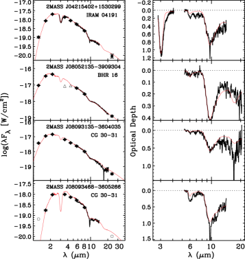
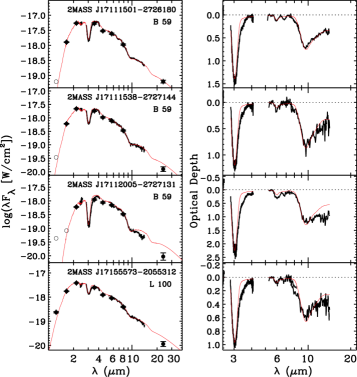
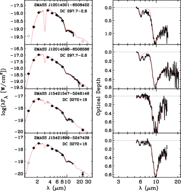
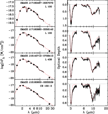
Figure 1.— Left panels: Observed ground-based and Spitzer/IRS spectra combined with broad band photometry (filled circles), and lower limits (open triangles) and 3$\sigma$ upper limits (open circles) thereof. The red line represents the fitted model (§4.1). The sources are sorted in increasing Right Ascension. The name of the background stars and the cores they trace are indicated. Right panels: Optical depth spectra, derived using the continuum models of the left panels, excluding the modeled ice and silicate features. Note the large variation of the relative depths of the 3.0 and 9.7 ${\rm\mu m}$ bands. The red line indicates the modeled H₂O ice and silicates spectrum. For clarity, error bars of the spectral data points are not shown.

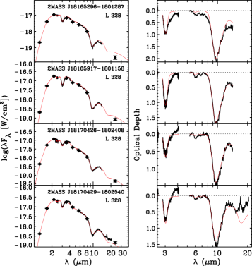
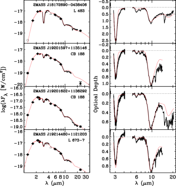
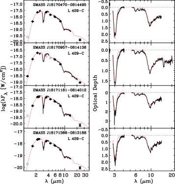
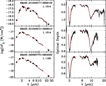
Figure 1.— (Continuation)

Table 2Model Spectra 

Spectral Type	$T_{\rm eff}$	log(g)
	K
G8 III	5000	2.50
K0 III	4500	2.50
K3 III	4500	2.00
K4 III	4250	2.00
K5 III	4000	2.00
K7 III	4000	1.50
M0 III	3700	1.00
M1 III	3500	1.00
M3 III	3200	1.00
M6 III	3200	0.50
M7 III	3000	0.50
M8 III	2800	0.50
M9 III	2500	0.50

Note. — Spectral types were assigned using polynomial fits to empirical $T_{\rm eff}$ and log(g) data following the method of Kane & Sahu (2003).

$\chi^{2}$ values were derived for all available observables, including photometric points, ground-based spectra and Spitzer spectra, except for those for which it is a priori known that insufficient information is available: the 3.1-3.7 ${\rm\mu m}$ spectral region (long-wavelength wing 3.0 ${\rm\mu m}$ band), the 5.3-7.1 ${\rm\mu m}$ region (6.0 and 6.85 ${\rm\mu m}$ ice bands), and the IRAC2 photometric point (4.67 ${\rm\mu m}$ CO ice band). The MIPS1 photometric point was not fitted either, to avoid too much weight to the longer wavelengths, which are not important for the ice bands studied here (although, in practice, the final models are in quite good agreement with the MIPS1 photometry; Fig. 1). Because there are many more spectroscopic than photometric data points, the latter would have much larger $\chi^{2}$ values. Thus the spectroscopic $\chi^{2}$ values were divided by the number of data points and then the “reduced $\chi^{2}$ values” of the different observables were averaged to represent the goodness of fit over all observables. In addition, a reduced $\chi^{2}$ value was derived for the most crucial observables for spectral type determination: near-infrared photometry, the shape of near-infrared spectra and the 4.0-4.1 ${\rm\mu m}$ spectral region. The reduced $\chi^{2}$ values and parameters of the best fits are reported in Table 3 and the fits are plotted in Fig. 1 (red lines in the left panels). Good fits are often obtained. In seven cases, the reduced $\chi^{2}$ values exceed 3 and the main cause for that is indicated in the notes of Table 3. Typically, the relative scalings of the K-band photometry, and the (partial) K-band and L-band spectra deviate from the model, but the fits are good at longer wavelengths.

In seven other cases, no spectra below 5 ${\rm\mu m}$, and thus no independent measures of spectral type and $N$(H₂O) were available (Table 1). This most strongly affects the $N$(H₂O) determination, as the depth of the 13 ${\rm\mu m}$ libration mode is degenerate with the slope of the applied extinction curve and the assumed silicate band profiles. An uncertainty in the spectral type affects the shape and depth of the 5-8 ${\rm\mu m}$ absorption features because of photospheric features that emerge for spectral types later than M1 III. In practice, the 8 ${\rm\mu m}$ photospheric SiO bands can be used to constrain the spectral type sufficiently well, however.

Table 3Continuum Fit Parameters 

Source	Spectral Type	$A_{\rm K}$	$\tau_{3.0}$	$\tau_{\rm 9.7}$	$\chi_{\nu}^{2}$(total)	$\chi_{\nu}^{2}$(SpT)
2MASS J		mag
$04215402+1530299$	K0 (G8-K5)	3.04 (0.09 )	1.09 (0.05)	0.88 (0.04 )	1.20	1.93
$08052135-3909304$	M0 (K5-M1)g	1.47 (0.04 )	$<$0.70h	0.41 (0.02 )	0.29	$\cdots$ j
$08093135-3604035$	K0 (G8-M1)g	1.89 (0.06 )	0.55h (0.25)	0.58 (0.02 )	0.42	$\cdots$ j
$08093468-3605266$	M3 (M0-M7)g	4.52 (0.14 )	2.10h (0.42)	0.95 (0.04 )	0.58	$\cdots$ j
$12014301-6508422$	M3 (M3-M7)g	5.17 (0.15 )	3.20h (0.80)	1.35 (0.05 )	1.94	$\cdots$ j
$12014598-6508586$	K3 (G8-K7)g	3.07 (0.09 )	1.45h (0.25)	0.78 (0.03 )	0.37	$\cdots$ j
$15421547-5248146$	M0 (K7-M1)g	1.94 (0.06 )	$<$0.70h	0.81 (0.03 )	0.51	$\cdots$ j
$15421699-5247439$	K7 (K5-M3)g	2.87 (0.09 )	0.85h (0.25)	0.84i (0.03 )	0.26	$\cdots$ j
$17111501-2726180$	M6 (M3-M6)	3.91 (0.12 )	1.39 (0.07)	0.76 (0.03 )	1.21	1.92
$17111538-2727144$	M3 (M1-M6)	3.53 (0.11 )	1.20 (0.06)	0.87 (0.03 )	1.96	1.69
$17112005-2727131$	M3 (M1-M3)	6.00 (0.18 )	2.25 (0.11)	1.30 (0.05 )	4.91k	5.22
$17155573-2055312$	M1 (M0-M1)	2.65 (0.08 )	0.97 (0.05)	0.66 (0.03 )	1.57	1.94
$17160467-2057072$	K7 (K7-M0)	3.24 (0.10 )	1.27 (0.06)	0.77 (0.03 )	9.38k	3.42
$17160860-2058142$	G8 (G8-K4)	2.45 (0.07 )	0.91 (0.05)	0.77 (0.08 )	0.72	1.28
$18140712-0708413$	K7 (K5-M0)	1.89 (0.06 )	0.83 (0.04)	0.60 (0.02 )	0.64	0.72
$18160600-0225539$	M0 (M0-M1)	1.25 (0.04 )	0.63 (0.09)	0.50 (0.02 )	1.77	1.76
$18165296-1801287$	M1	3.00 (0.18 )	0.96 (0.10)	2.00 (0.12 )	1.21	1.34
$18165917-1801158$	M6 (M3-M6)	3.34 (0.10 )	1.10 (0.05)	1.66 (0.07 )	0.76	1.10
$18170426-1802408$	M6 (M3-M6)	2.50 (0.08 )	0.65 (0.03)	1.38 (0.06 )	1.89	4.22
$18170429-1802540$	M1 (M0-M1)	2.96 (0.09 )	0.85 (0.09)	1.40 (0.06 )	2.07	1.92
$18170470-0814495$	M0 (M0-M1)	4.27 (0.13 )	2.33 (0.12)	1.39 (0.06 )	12.28k	2.49
$18170957-0814136$	M1 (M1-M6)	3.27 (0.10 )	1.69 (0.08)	1.04 (0.04 )	2.02	2.49
$18171181-0814012$	K7 (K5-M0)	4.31 (0.13 )	2.26 (0.11)	1.49 (0.06 )	2.00	1.11
$18171366-0813188$	K7 (K5-M0)	3.58 (0.11 )	2.02 (0.10)	1.17 (0.05 )	16.21k	1.93
$18172690-0438406$	M3 (M1-M6)	4.60 (0.14 )	2.55 (0.13)	1.11 (0.04 )	4.53k	0.78
$19201597+1135146$	M1 (M0-M1)	3.14 (0.09 )	0.79 (0.04)	1.05 (0.04 )	1.01	0.69
$19201622+1136292$	M6 (M3-M6)	2.50 (0.13 )	0.60 (0.03)	0.78 (0.03 )	0.99	1.11
$19214480+1121203$	M6 (M3-M6)	2.10 (0.06 )	0.85 (0.04)	0.95 (0.04 )	7.31k	1.74
$21240517+4959100$	M1 (M0-M1)	3.10 (0.09 )	1.30 (0.06)	0.95 (0.04 )	1.03	0.82
$21240614+4958310$	K4 (K4-K5)	1.60 (0.05 )	0.58 (0.03)	0.52 (0.02 )	1.35	1.33
$22063773+5904520$	G8	1.74 (0.09 )	0.67 (0.03)	0.33 (0.01 )	2.95	2.48
$04393886+2611266$	K7 (K5-M1)	3.00 (0.09 )	1.42 (0.07)	0.84 (0.03 )	0.80	2.61
$18300061+0115201$	M3 (M3-M6)	6.38 (0.19 )	1.81 (0.09)	1.71 (0.07 )	7.30k	18.79

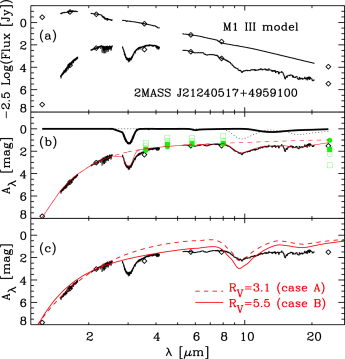
Figure 2.— Derivation of an extinction curve for the star 2MASS J21240517+4959100 behind L1014. Panel (a) shows the observed spectrum, broad-band photometry (diamonds) and an M1 III model spectrum. After subtracting these spectra on a Log scale, the resulting extinction curve is shown in panel (b). The solid red line is the result of adding spectra of solid H₂O (thick solid black line) and silicate features (dotted black line) to a polynomial fit. The dashed line then represents the feature-free extinction curve used in the background star continuum fits. Green symbols represent the average extinction in broad band filters derived from nearby cloud observations (Chapman et al. 2009) for lines of sight with $A_{\rm K}<0.5$ (open squares), $0.5<A_{\rm K}<1.0$ (open circles), $1.0<A_{\rm K}<2.0$ (filled squares), and $1.0<A_{\rm K}<2.0$ (filled circles). Panel (c) compares the empirical extinction curve with the calculated curves of $R_{\rm V}$=3.1 (case A) and 5.5 (case B) from Weingartner & Draine (2001).

4.2. The “High Resolution” Extinction Curve

Table 4Polynomial Coefficients of Feature-Free Extinction Curve (Eq. 2) 

Coefficient	Value
a0	0.5924
a1	-1.8235
a2	-1.3020
a3	5.9936
a4	-5.3429
a5	1.2619
a6	0.2738
a7	0.0069
a8	-0.0554

The background star spectra can be used to derive a high resolution extinction curve, in which the ice and dust features can be separated from the continuum extinction and in which large interpolations usually applied between, e.g., the IRAC 8 ${\rm\mu m}$ and MIPS 24 ${\rm\mu m}$ photometric data points are avoided. 2MASS J21240517+4959100 behind the core L1014 was chosen for this purpose, because high quality near-infrared spectra are available, indicating an accurate spectral type of M1 III. The extinction curve was derived as follows:

$$A_{\lambda}{\rm[mag]}=-2.5{\rm Log}(F_{\lambda}{\rm(obs)}/F_{\lambda}{\rm(model)}).$$ (1)

The absolute scaling of $F_{\lambda}{\rm(model)}$ is unknown, because there are no measurements of the star’s distance. To circumvent this problem, the model was scaled with respect to the observed spectrum such that the derived $A_{\lambda}$ follows known near-infrared extinction curves (i.e., $A_{\lambda}\propto\lambda^{-1.8}$; e.g., Indebetouw et al. 2005). This provides the “high-resolution” extinction curve shown in Fig. 2b. This curve is remarkably flat. At an $A_{\rm K}$ of 3.02 mag, the extinction is still 1.5 mag at 25 ${\rm\mu m}$. This confirms the results of Chapman et al. (2009), as indicated by the symbols in Fig. 2b, and McClure (2009). Subsequently, continuum and feature extinction were separated by adding a laboratory spectrum of solid H₂O (at $T=10$ K; Hudgins et al. 1993) and a silicates model spectrum (§4.1) to a polynomial fit to feature-free regions of the form

$${\rm Log}(A_{\lambda}/A_{\rm K})=a_{0}+a_{1}{\rm Log(}\lambda)+a_{2}{\rm[{\rm Log}(}\lambda)]^{2}+...~{}$$ (2)

with $\lambda$ in ${\rm\mu m}$ and $A_{\lambda}$ in magnitude. The polynomial coefficients are listed in Table 4, and the curve is plotted with a dashed red line in Fig. 2b. This feature-free extinction curve works well for most sources. Examples of exceptions might be 2MASS J19201597+1135146 (model too shallow $>10$ ${\rm\mu m}$) and 2MASS J18172690-0438406 (model too steep $>10$ ${\rm\mu m}$), but no systematic trend with $A_{\rm K}$ or core environment could be found. In these cases the silicate model used in the fits may be responsible for the deviations as well.

Table 5Optical Depths 5-8 ${\rm\mu m}$ Features [publish electronically] 

Source	$\tau_{\rm int}$ [cm-1]				$\tau_{\rm 6.0}$	$\tau_{\rm 6.85}$	$\tau_{\rm C1}$	$\tau_{\rm C2}$	$\tau_{\rm C3}$	$\tau_{\rm C4}$	$\tau_{\rm C5}$
	5.2-6.4 ${\rm\mu m}$	5.2-6.4 ${\rm\mu m}$	6.4-7.2 ${\rm\mu m}$	6.4-7.2 ${\rm\mu m}$
2MASS J		minus H2O		minus H2O
$04215402+1530299$	26.27 (1.96)	14.06 (1.96)	17.48 (2.69)	12.44 (2.69)	0.19 (0.04)	0.15 (0.07)	0.08 (0.01)	0.09 (0.01)	0.10 (0.03)	0.08 (0.03)	0.00 (0.05)
$08052135-3909304$	6.57 (0.94)	-1.26 (0.94)	7.54 (1.10)	4.31 (1.10)	0.05 (0.02)	0.06 (0.03)	0.00 (0.01)	0.00 (0.01)	0.03 (0.01)	0.03 (0.01)	0.00 (0.02)
$08093135-3604035$	10.44 (1.02)	4.30 (1.02)	9.36 (2.68)	6.83 (2.68)	0.10 (0.02)	0.09 (0.03)	0.01 (0.01)	0.04 (0.01)	0.05 (0.01)	0.04 (0.01)	0.00 (0.03)
$08093468-3605266$	50.63 (1.71)	27.16 (1.71)	22.61 (2.24)	12.94 (2.24)	0.33 (0.04)	0.17 (0.05)	0.14 (0.01)	0.18 (0.01)	0.09 (0.02)	0.08 (0.02)	0.00 (0.04)
$12014301-6508422$	49.01 (1.05)	13.22 (1.05)	19.23 (1.32)	4.49 (1.32)	0.33 (0.02)	0.19 (0.04)	0.02 (0.01)	0.12 (0.01)	0.10 (0.02)	0.00 (0.01)	0.00 (0.04)
$12014598-6508586$	26.41 (1.09)	10.20 (1.09)	20.76 (1.38)	14.08 (1.38)	0.18 (0.02)	0.16 (0.04)	0.07 (0.01)	0.06 (0.01)	0.13 (0.02)	0.07 (0.01)	0.00 (0.03)
$15421547-5248146$	8.36 (2.18)	0.54 (2.18)	6.47 (2.54)	3.25 (2.54)	0.06 (0.04)	0.07 (0.06)	0.01 (0.01)	0.00 (0.02)	0.03 (0.02)	0.00 (0.03)	0.00 (0.05)
$15421699-5247439$	15.41 (1.26)	5.90 (1.26)	12.40 (1.65)	8.49 (1.65)	0.11 (0.03)	0.10 (0.04)	0.07 (0.01)	0.01 (0.01)	0.06 (0.02)	0.06 (0.02)	0.00 (0.03)
$17111501-2726180$	18.76 (0.64)	3.17 (0.64)	13.70 (0.80)	7.28 (0.80)	0.14 (0.01)	0.12 (0.02)	0.03 (0.01)	0.02 (0.01)	0.09 (0.01)	0.03 (0.01)	0.00 (0.02)
$17111538-2727144$	24.14 (2.75)	10.77 (2.75)	8.11 (3.48)	2.60 (3.48)	0.20 (0.06)	0.08 (0.09)	0.06 (0.02)	0.05 (0.02)	0.01 (0.04)	0.03 (0.04)	0.00 (0.07)
$17112005-2727131$	46.71 (1.95)	21.56 (1.95)	20.81 (2.21)	10.44 (2.21)	0.30 (0.04)	0.20 (0.06)	0.11 (0.01)	0.13 (0.01)	0.13 (0.02)	0.04 (0.02)	0.00 (0.04)
$17155573-2055312$	14.83 (1.60)	4.00 (1.60)	8.26 (1.97)	3.80 (1.97)	0.11 (0.03)	0.08 (0.05)	0.04 (0.01)	0.02 (0.01)	0.06 (0.02)	0.00 (0.02)	0.00 (0.04)
$17160467-2057072$	14.30 (2.48)	0.15 (2.48)	19.51 (3.38)	13.67 (3.38)	0.10 (0.05)	0.18 (0.08)	0.00 (0.02)	0.01 (0.02)	0.11 (0.03)	0.10 (0.03)	0.00 (0.07)
$17160860-2058142$	11.18 (1.31)	1.00 (1.31)	7.75 (1.78)	3.55 (1.78)	0.08 (0.03)	0.08 (0.05)	0.00 (0.01)	0.01 (0.01)	0.05 (0.02)	0.01 (0.02)	0.00 (0.03)
$18140712-0708413$	13.30 (1.77)	3.98 (1.77)	10.78 (1.61)	6.94 (1.61)	0.09 (0.03)	0.07 (0.04)	0.02 (0.01)	0.04 (0.01)	0.04 (0.02)	0.04 (0.02)	0.00 (0.04)
$18160600-0225539$	14.64 (1.66)	7.60 (1.66)	11.23 (2.21)	8.33 (2.21)	0.10 (0.03)	0.09 (0.06)	0.05 (0.01)	0.04 (0.01)	0.04 (0.02)	0.06 (0.02)	0.00 (0.04)
$18165296-1801287$	19.54 (0.92)	8.81 (0.92)	8.00 (1.24)	3.58 (1.24)	0.13 (0.02)	0.09 (0.03)	0.04 (0.01)	0.06 (0.01)	0.06 (0.01)	0.01 (0.01)	0.00 (0.03)
$18165917-1801158$	24.64 (1.05)	12.37 (1.05)	12.63 (1.22)	7.58 (1.22)	0.17 (0.02)	0.11 (0.03)	0.05 (0.01)	0.10 (0.01)	0.08 (0.01)	0.04 (0.01)	0.00 (0.02)
$18170426-1802408$	23.25 (1.18)	15.98 (1.18)	14.30 (1.46)	11.31 (1.46)	0.17 (0.02)	0.10 (0.04)	0.07 (0.01)	0.12 (0.01)	0.08 (0.01)	0.06 (0.02)	0.00 (0.03)
$18170429-1802540$	17.86 (2.29)	8.34 (2.29)	9.63 (2.10)	5.72 (2.10)	0.13 (0.05)	0.09 (0.05)	0.03 (0.01)	0.07 (0.02)	0.06 (0.02)	0.04 (0.02)	0.00 (0.05)
$18170470-0814495$	40.68 (1.48)	14.60 (1.48)	23.81 (1.85)	13.06 (1.85)	0.28 (0.03)	0.21 (0.05)	0.11 (0.01)	0.07 (0.01)	0.15 (0.02)	0.06 (0.02)	0.00 (0.04)
$18170957-0814136$	27.44 (1.10)	8.56 (1.10)	18.09 (1.22)	10.31 (1.22)	0.19 (0.02)	0.16 (0.03)	0.07 (0.01)	0.03 (0.01)	0.11 (0.01)	0.06 (0.01)	0.00 (0.02)
$18171181-0814012$	41.27 (1.68)	15.97 (1.68)	26.33 (2.23)	15.90 (2.23)	0.28 (0.04)	0.23 (0.06)	0.12 (0.01)	0.07 (0.01)	0.15 (0.02)	0.11 (0.02)	0.00 (0.04)
$18171366-0813188$	34.05 (1.63)	11.50 (1.63)	25.80 (2.12)	16.50 (2.12)	0.24 (0.04)	0.21 (0.06)	0.08 (0.01)	0.06 (0.01)	0.15 (0.02)	0.10 (0.02)	0.00 (0.04)
$18172690-0438406$	52.65 (1.15)	24.10 (1.15)	28.26 (1.34)	16.49 (1.34)	0.34 (0.03)	0.23 (0.04)	0.14 (0.01)	0.15 (0.01)	0.16 (0.02)	0.09 (0.01)	0.00 (0.03)
$19201597+1135146$	14.91 (1.20)	6.04 (1.20)	10.25 (1.72)	6.59 (1.72)	0.10 (0.03)	0.09 (0.04)	0.03 (0.01)	0.04 (0.01)	0.08 (0.02)	0.04 (0.02)	0.00 (0.04)
$19201622+1136292$	11.74 (0.76)	5.00 (0.76)	4.40 (0.77)	1.62 (0.77)	0.09 (0.01)	0.05 (0.02)	0.04 (0.01)	0.03 (0.01)	0.03 (0.01)	0.00 (0.01)	0.00 (0.02)
$19214480+1121203$	19.51 (1.72)	10.01 (1.72)	10.35 (2.22)	6.43 (2.22)	0.15 (0.04)	0.09 (0.06)	0.04 (0.01)	0.08 (0.01)	0.02 (0.02)	0.06 (0.02)	0.00 (0.04)
$21240517+4959100$	19.44 (1.23)	4.93 (1.23)	13.95 (1.31)	7.97 (1.31)	0.13 (0.02)	0.14 (0.03)	0.03 (0.01)	0.02 (0.01)	0.12 (0.01)	0.02 (0.01)	0.00 (0.02)
$21240614+4958310$	8.54 (1.26)	2.01 (1.26)	8.12 (1.54)	5.44 (1.54)	0.08 (0.03)	0.08 (0.04)	0.00 (0.01)	0.02 (0.01)	0.03 (0.02)	0.06 (0.02)	0.00 (0.03)
$22063773+5904520$	10.22 (1.31)	2.70 (1.31)	9.70 (1.73)	6.61 (1.73)	0.09 (0.03)	0.08 (0.05)	0.00 (0.01)	0.03 (0.01)	0.05 (0.02)	0.05 (0.02)	0.00 (0.03)
$04393886+2611266$	20.66 (0.22)	4.78 (0.22)	13.48 (0.29)	6.93 (0.29)	0.15 (0.01)	0.12 (0.01)	0.03 (0.01)	0.02 (0.01)	0.08 (0.01)	0.04 (0.01)	0.00 (0.01)
$18300061+0115201$	33.96 (1.25)	13.77 (1.25)	20.82 (0.89)	12.51 (0.89)	0.26 (0.03)	0.20 (0.02)	0.10 (0.01)	0.08 (0.01)	0.14 (0.01)	0.08 (0.01)	0.00 (0.03)

Note. — Uncertainties in parentheses based on statistical errors in the spectra only, unless noted otherwise below.

Table 6Column Densities of the Ices 

Source	$N$(H2O)	$N$(NH${}_{4}^{+}$)		$N$(CO2)		$N$(CH3OH)		$N$(HCOOH)		$N$(CH4)		$N$(NH3)
2MASS J	$10^{18}$	$10^{17}$		$10^{17}$		$10^{17}$		$10^{17}$		$10^{17}$		$10^{17}$
	${\rm cm^{-2}}$	${\rm cm^{-2}}$	%H2O	${\rm cm^{-2}}$	%H2O	${\rm cm^{-2}}$	%H2O	${\rm cm^{-2}}$	%H2O	${\rm cm^{-2}}$	%H2O	${\rm cm^{-2}}$	%H2O
$04215402+1530299$	1.84 (0.20)	2.73 (0.61)	14.80 (3.71)	$\cdots$	$\cdots$	$<$1.55	$<$9.46	$<$0.98	$<$6.03	$<$1.54	$<$9.45	$<$5.46	$<$33.38
$08052135-3909304$	$<$1.18	0.98 (0.24)	$>$8.29	3.79	$>$32.11	$<$0.50	$\cdots$	$<$0.23	$\cdots$	$<$1.02	$\cdots$	$<$2.00	$\cdots$
$08093135-3604035$	0.92 (0.42)	1.55 (0.60)	16.71 (10.1)	$<$11.31	$<$226.0	$<$2.00	$<$39.97	$<$0.23	$<$4.61	$<$2.15	$<$43.03	$<$3.00	$<$59.95
$08093468-3605266$	3.54 (0.79)	2.94 (0.50)	8.29 (2.34)	$\cdots$	$\cdots$	$<$10.00	$<$36.34	$<$1.63	$<$5.94	$<$1.86	$<$6.79	$<$4.13	$<$15.04
$12014301-6508422$	5.40 (1.45)	1.02 (0.30)	1.89 (0.75)	$\cdots$	$\cdots$	$<$8.52	$<$21.59	$<$0.29	$<$0.75	$<$1.15	$<$2.92	$<$9.00	$<$22.80
$12014598-6508586$	2.44 (0.48)	3.20 (0.31)	13.07 (2.87)	8.34 (1.91)	34.11 (10.3)	$<$2.00	$<$10.18	$<$0.81	$<$4.17	$<$1.01	$<$5.17	$<$4.00	$<$20.36
$15421547-5248146$	$<$1.18	0.73 (0.57)	$>$6.25	$\cdots$	$\cdots$	$<$5.34	$\cdots$	$<$0.44	$\cdots$	$<$2.03	$\cdots$	$<$3.64	$\cdots$
$15421699-5247439$	1.43 (0.44)	1.92 (0.37)	13.45 (4.88)	$\cdots$	$\cdots$	$<$2.74	$<$27.62	$<$0.81	$<$8.22	$<$2.08	$<$20.99	$<$4.06	$<$40.83
$17111501-2726180$	2.35 (0.26)	1.52 (0.18)	6.49 (1.06)	$\cdots$	$\cdots$	$<$1.60	$<$7.65	$<$0.35	$<$1.70	$<$0.57	$<$2.75	$<$1.32	$<$6.32
$17111538-2727144$	2.01 (0.22)	$<$2.37	$<$13.24	$\cdots$	$\cdots$	$<$2.00	$<$11.15	$<$0.76	$<$4.27	$<$2.58	$<$14.41	$<$3.00	$<$16.73
$17112005-2727131$	3.79 (0.42)	2.17 (0.50)	5.71 (1.46)	$\cdots$	$\cdots$	$<$2.00	$<$5.92	$<$1.34	$<$3.99	$<$1.39	$<$4.14	$<$9.00	$<$26.68
$17155573-2055312$	1.63 (0.18)	0.77 (0.44)	4.74 (2.79)	$\cdots$	$\cdots$	$<$0.86	$<$5.94	$<$0.42	$<$2.90	$<$1.41	$<$9.71	$<$4.00	$<$27.54
$17160467-2057072$	2.13 (0.23)	2.99 (0.76)	13.99 (3.91)	$\cdots$	$\cdots$	$<$1.39	$<$7.32	$<$0.58	$<$3.09	$<$1.81	$<$9.54	$<$4.00	$<$21.06
$17160860-2058142$	1.53 (0.17)	0.72 (0.40)	4.72 (2.69)	$\cdots$	$\cdots$	$<$0.43	$<$3.17	$<$0.31	$<$2.32	$<$1.10	$<$8.10	$<$4.00	$<$29.30
$18140712-0708413$	1.40 (0.15)	1.40 (0.36)	9.99 (2.83)	$\cdots$	$\cdots$	0.70 (0.20)	4.97 (1.52)	$<$0.30	$<$2.46	$<$1.05	$<$8.45	$<$3.50	$<$27.99
$18160600-0225539$	1.06 (0.19)	1.83 (0.50)	17.29 (5.65)	$\cdots$	$\cdots$	$<$0.76	$<$8.73	$<$0.56	$<$6.47	$<$1.64	$<$18.86	$<$3.50	$<$40.18
$18165296-1801287$	1.62 (0.22)	0.72 (0.28)	4.48 (1.84)	$\cdots$	$\cdots$	$<$1.36	$<$9.82	$<$0.48	$<$3.49	$<$1.20	$<$8.62	$<$2.48	$<$17.87
$18165917-1801158$	1.85 (0.20)	1.62 (0.27)	8.76 (1.78)	$\cdots$	$\cdots$	$<$0.85	$<$5.21	$<$0.56	$<$3.43	$<$0.71	$<$4.36	$<$3.32	$<$20.22
$18170426-1802408$	1.09 (0.12)	2.51 (0.33)	22.90 (3.96)	$\cdots$	$\cdots$	$<$0.83	$<$8.60	$<$0.83	$<$8.61	$<$0.96	$<$9.85	$<$3.72	$<$38.23
$18170429-1802540$	1.43 (0.20)	1.22 (0.47)	8.52 (3.53)	3.37 (1.95)	23.55 (14.0)	$<$0.77	$<$6.29	$<$0.37	$<$3.05	$<$0.90	$<$7.32	$<$3.67	$<$29.82
$18170470-0814495$	3.93 (0.44)	2.41 (0.42)	6.13 (1.26)	$\cdots$	$\cdots$	2.49 (0.60)	6.34 (1.69)	$<$1.28	$<$3.66	$<$1.80	$<$5.14	$<$7.00	$<$20.00
$18170957-0814136$	2.85 (0.31)	1.82 (0.27)	6.39 (1.20)	12.29 (1.29)	43.12 (6.63)	2.69 (0.58)	9.46 (2.30)	$<$0.89	$<$3.53	$<$0.97	$<$3.84	$<$3.16	$<$12.48
$18171181-0814012$	3.81 (0.42)	2.80 (0.50)	7.35 (1.55)	$\cdots$	$\cdots$	4.42 (0.86)	11.58 (2.60)	$<$1.48	$<$4.38	$<$1.42	$<$4.19	$<$6.71	$<$19.80
$18171366-0813188$	3.40 (0.38)	3.09 (0.48)	9.08 (1.74)	$\cdots$	$\cdots$	3.48 (0.86)	10.24 (2.78)	$<$0.99	$<$3.29	$<$1.24	$<$4.12	$<$4.83	$<$15.97
$18172690-0438406$	4.31 (0.48)	3.02 (0.30)	7.01 (1.05)	18.86 (1.72)	43.75 (6.31)	3.63 (0.65)	8.44 (1.79)	$<$1.63	$<$4.28	$<$0.95	$<$2.48	$<$7.00	$<$18.28
$19201597+1135146$	1.34 (0.14)	1.42 (0.39)	10.64 (3.14)	$\cdots$	$\cdots$	$<$0.70	$<$5.95	$<$0.37	$<$3.12	$<$1.15	$<$9.69	$<$6.58	$<$55.33
$19201622+1136292$	1.01 (0.11)	0.31 (0.17)	3.09 (1.74)	3.86 (1.07)	38.08 (11.3)	$<$0.70	$<$7.77	$<$0.50	$<$5.58	$<$0.58	$<$6.49	$<$2.00	$<$22.15
$19214480+1121203$	1.43 (0.16)	1.38 (0.50)	9.65 (3.68)	$\cdots$	$\cdots$	$<$1.61	$<$12.64	$<$0.49	$<$3.88	$<$1.63	$<$12.85	$<$2.57	$<$20.22
$21240517+4959100$	2.19 (0.24)	1.48 (0.29)	6.76 (1.55)	8.24 (2.69)	37.60 (13.0)	1.54 (0.38)	7.04 (1.90)	$<$0.40	$<$2.07	$<$1.83	$<$9.43	$<$4.20	$<$21.57
$21240614+4958310$	0.98 (0.11)	1.18 (0.34)	12.01 (3.78)	$\cdots$	$\cdots$	$<$0.59	$<$6.83	$<$0.27	$<$3.13	$<$1.14	$<$13.04	$<$2.50	$<$28.57
$22063773+5904520$	1.13 (0.12)	1.44 (0.39)	12.70 (3.74)	$\cdots$	$\cdots$	$<$0.40	$<$3.98	$<$0.31	$<$3.10	$<$1.11	$<$11.02	$<$2.30	$<$22.82
$04393886+2611266$	2.39 (0.26)	1.44 (0.06)	6.03 (0.72)	7.11 (0.05)	29.66 (3.32)	$<$0.25	$<$1.17	$<$0.38	$<$1.81	$<$0.82	$<$3.84	$<$1.45	$<$6.85
$18300061+0115201$	3.04 (0.34)	2.68 (0.20)	8.79 (1.18)	11.93 (0.21)	39.14 (4.43)	$<$2.10	$<$7.75	$<$1.18	$<$4.36	$<$0.58	$<$2.14	$<$6.39	$<$23.61

Note. — Column densities were determined using the intrinsic integrated band strengths listed in Table 7. Uncertainties (1$\sigma$) are indicated in brackets and upper limits are of 3$\sigma$ significance.

Table 7Intrinsic Integrated Band Strengths 

Molecule	Mode	$A$	Reference
		cm/molecule
H2O	3.0 ${\rm\mu m}$  stretch	$2.0\times 10^{-16}$	Hagen et al. (1981)
NH${}_{4}^{+}$	6.8 ${\rm\mu m}$  deformation	$4.4\times 10^{-17}$	Schutte & Khanna (2003)
CO2	15.0 ${\rm\mu m}$ bend	$1.1\times 10^{-17}$	Gerakines et al. (1995)
CH3OH	3.53 ${\rm\mu m}$ C-H stretch	$5.6\times 10^{-18}$	Kerkhof et al. (1999)
CH3OH	9.7 ${\rm\mu m}$  O-H stretch	$1.6\times 10^{-17}$	Kerkhof et al. (1999)
HCOOH	5.85 ${\rm\mu m}$ C=O stretch	$6.7\times 10^{-17}$	Schutte et al. (1999)
HCOOH	7.25 ${\rm\mu m}$ C-H deformation	$2.6\times 10^{-18}$	Schutte et al. (1999)
CH4	7.68 ${\rm\mu m}$ deformation	$7.3\times 10^{-18}$	Boogert et al. (1997)
NH3	8.9 ${\rm\mu m}$  umbrella	$1.3\times 10^{-17}$	Kerkhof et al. (1999)

4.3. Absorption Band Strengths and Column Densities

The continuum fits, as indicated with red lines in Fig. 1 (left panels), but excluding modeled H₂O and silicate bands, were used to put the spectra on an optical depth scale. The right panels of Fig. 1 show that the optical depth in the 7.5-8.0 ${\rm\mu m}$ region is not always fully explained by the modeled H₂O and silicate bands. This may be related to inaccuracies in the applied extinction curve and stellar model. Therefore, in the subsequent analysis of the optical depth spectra, local straight line continua between 7.5 and 5.3 or 6.4 ${\rm\mu m}$ were used to correct for these small offsets (see Fig. 3 for examples).

Peak and integrated optical depths were determined for the 6.0 and 6.85 ${\rm\mu m}$ bands, before and after the O-H bending mode of H₂O was subtracted using an amorphous ice spectrum at $T$=10 K (Hudgins et al. 1993; Table 5). The features in the H₂O-subtracted spectra were also decomposed into the five components discussed in Boogert et al. (2008). These components (labeled “C1”-“C5”) are useful in characterizing source-to-source variations of the absorption in the 5-7 ${\rm\mu m}$ wavelength region (§4.4.6). They do not represent a unique decomposition, however, and each component may be the result of absorption by more than one molecular band. Examples of this decomposition are shown in Fig. 3. For comparison two YSOs are shown as well (Boogert et al., 2008). Clearly, the relative depths of the components vary considerably between background stars and between YSOs.

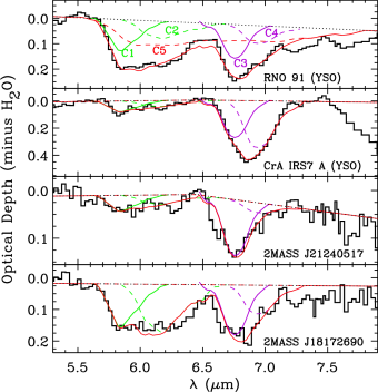
Figure 3.— Decomposition of the absorption features in the 5-8 ${\rm\mu m}$ spectra of two background stars (bottom panels), compared to two YSOs (Boogert et al., 2008) in the top panels. The components are labeled C1 (solid green), C2 (dashed green), C3 (solid purple), C4 (dashed purple), and C5 (dashed red). The sum of the components is indicated with a thick red line. Note that the relative strengths of the components (e.g., C3/C1) varies strongly toward both YSOs and background stars. Component C5 has not been detected toward any background star. All components are added to a local straight line continuum (dotted black line) to remove small inaccuracies from the global continuum fitting process.

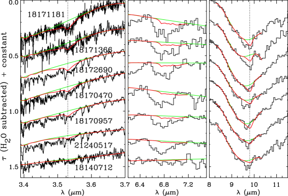
Figure 4.— Left panel: Sources with detections (top 2 sources) or tentative detections of the C-H stretching mode of solid CH₃OH at 3.53 ${\rm\mu m}$. The green line is the assumed local continuum and the red line the laboratory spectrum H₂O:CH₃OH:CO:NH₃=100:10:1:1 ($T=10$ K; Hudgins et al. 1993) corresponding to the column densities listed in Table 6. Middle panel: the 6.3-8.0 ${\rm\mu m}$ region of the same sources as in the left panel showing the C-H bending mode of CH₃OH (red) with the assumed local continuum (green) at the same column densities as in the left panel. The observed absorption is much deeper due to an overlapping band of (possibly) NH${}_{4}^{+}$ (§4.3). Right panel: the 8-11.5 ${\rm\mu m}$ region of the same sources as in the left panel showing the C-O stretching mode of CH₃OH (red) with the assumed local continuum (green) at the same column densities as in the left panel. Note that a scaling factor along the optical depth axis was applied for the spectra to fit in the panel.

Column densities were determined for solid H₂O, ${\rm NH_{4}^{+}}$, and CO₂ (Table 6), using the intrinsic integrated band strengths listed in Table 7. The H₂O column density is unreliable if no $L-$band spectrum is available (7 out of 31 sources), and the 13 ${\rm\mu m}$ libration mode is the main tracer. The depth of the latter is strongly affected by the assumed shape of the extinction curve and by overlapping stretching and bending modes of silicates. The ${\rm NH_{4}^{+}}$ column density is derived, assuming that the entire 6.85 ${\rm\mu m}$ band (i.e., both components “C3” and “C4” listed in Table 5) can be attributed to it, after correction for any overlapping bands of the C-H deformation mode of solid CH₃OH (see below). This identification has not been fully validated, however, because no other ${\rm NH_{4}^{+}}$ bands have been detected (Schutte & Khanna, 2003; Boogert et al., 2008). The identification of the 15.2 ${\rm\mu m}$ band is not disputed, and the solid CO₂ column density is listed for the 8 sources for which this wavelength range was observed. All CO₂ observations were done at a low resolving power of $\sim$90, which is insufficient to assess the composition or thermal processing history of the ices (Pontoppidan et al., 2008).

The background star spectra were also searched for CH₃OH, HCOOH, NH₃ and CH₄ species that are often detected toward YSOs. For solid CH₃OH, the 3.53 ${\rm\mu m}$ C–H stretching and the 9.7 ${\rm\mu m}$ C–O stretching modes are usually used for column density determinations (Boogert et al., 2008; Bottinelli et al., 2010). The 3.53 ${\rm\mu m}$ band is preferred because it is free from interfering strong bands. Nevertheless it overlaps with the 3.47 ${\rm\mu m}$ band of hydrocarbons (Allamandola et al., 1992; Brooke et al., 1996) or NH₃ hydrates (Dartois & d’Hendecourt, 2001), as well as several photospheric lines. Thus, the most certain detections of solid CH₃OH are toward background stars that show a distinct 3.53 ${\rm\mu m}$ band. Fig. 4 shows that this is the case for certainly two lines of sight: 2MASS J18171181-0814012 and 2MASS J18171366-0813188. The strongest detection (2MASS J18171181-0814012) was verified by observations in two different observing runs, using two different telluric standard stars. A good agreement is found for the strength of the 9.7 ${\rm\mu m}$ band. Five additional lines of sight likely show solid CH₃OH as well, although in these cases the 3.53 ${\rm\mu m}$ feature is not as distinct from other fluctuations in the surrounding spectra (Fig. 4). For all of these 7 sources the CH₃OH abundance relative to H₂O is in the 5-12% range. A similar number of sources have upper limits of comparable magnitude, and thus the CH₃OH abundance varies in different environments.

For the YSOs studied in Boogert et al. (2008), HCOOH is considered a detection only if the 7.25 ${\rm\mu m}$ C-H deformation mode has been detected. This is not the case for any of the background stars. Based on the strength of the C1 component (Table 5), which may mostly be due to the C=O stretch mode of HCOOH, the abundance can in many lines of sight be constrained to less than or comparable to the typical detections toward YSOs of 2–5% relative to H₂O, however (Table 6).

Finally, for NH₃ and CH₄ the 8.9 ${\rm\mu m}$ umbrella and 7.68 ${\rm\mu m}$ bending modes are used to determine column density upper limits. For CH₄ the upper limits are sometimes comparable but rarely less than the detections of $\sim$4% toward YSOs (Öberg et al., 2008). For NH₃ the upper limits are typically $\sim$20% relative to H₂O (Table 6), and are thus not significant compared to the detections of 2-15% toward YSOs (Bottinelli et al., 2010).

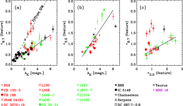
Figure 5.— Correlation plots of $A_{\rm K}$ with the peak optical depth of the 9.7 ${\rm\mu m}$ feature (a), of $A_{\rm K}$ with the peak optical depth of the 3.0 ${\rm\mu m}$ feature (b), and of the peak optical depths of the 3.0 and 9.7 ${\rm\mu m}$ features (c). Background stars tracing different clouds and cores are indicated with different symbols and colors. Solid black lines show least-square fits to all data points, excluding the ones strongly affected by diffuse medium absorption (L328) and the ones in the Taurus and Serpens molecular clouds. The fit in panel (a) was only done for $A_{\rm K}>1.4$ mag. The dashed line in that panel is the diffuse medium relation taken from the literature (Whittet, 2003), and the values for the B68, IC 5146, Chamaeleon, and most Serpens and Taurus sources were taken from Chiar et al. (2007).

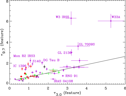
Figure 6.— Peak optical depths of the 3.0 and 9.7 ${\rm\mu m}$ absorption features for both background stars (in black, red and green; see legend of Fig. 5) and YSOs (purple asterisks). Only YSOs with reliable 3 ${\rm\mu m}$ spectra are plotted. The solid line represents the fit for background stars as derived in Fig. 5 panel (c). YSOs deviating more than 3$\sigma$ from the solid line are labeled, except for IC 1396 $\alpha$ and B5 IRS1 (both above the solid line), and IRAS 03439, L1448 IRS1 (below the solid line), which are not labeled to avoid crowding in the plot.

4.4. Correlation Plots

To facilitate the analysis of the observational parameters in many sight-lines in many different environments (quiescent core and cloud media, low mass YSOs, massive YSOs), a number of correlation plots are presented below. The values for the YSOs were taken from Boogert et al. (2008) and Reach et al. (2009). Note that in plots involving $A_{\rm K}$ no YSOs are present because of the unknown shape of the intrinsic K-band continuum emission. Also, background stars with $\tau_{3.0}$ upper limits have been excluded from the plots.

4.4.1 $\tau_{9.7}$ versus $A_{\rm K}$

The plot of the peak optical depth of the 9.7 ${\rm\mu m}$ band of silicates against K-band continuum extinction $A_{\rm K}$ shows an interesting behavior (Fig. 5a). While at low $A_{\rm K}$ the diffuse medium relation (Whittet, 2003)

$$\tau_{9.7}=0.554\times A_{\rm K}~{}$$ (3)

is followed (assuming $A_{\rm V}/A_{\rm K}$=8.8), a less steep relation is observed at $A_{\rm K}\geq$1 mag in dense sight-lines. This was discovered by Chiar et al. (2007) in the IC 5146, B68 and B59 cores and Serpens and Taurus clouds, and here this behavior is extended in more lines of sight, at higher K-band extinctions. Some background stars, however, follow the diffuse medium correlation, most notably those behind L328, and, as noted by Chiar et al. (2007), one source behind Serpens (2MASS J18285266+0028242). Thus, in these lines of sight the extinction may well be dominated by diffuse rather than dense dust. Excluding these particular background stars, a polynomial was fitted to objects with $A_{\rm K}>$1.4 mag:

$$\tau_{9.7}=(0.12\pm 0.05)+(0.21\pm 0.02)\times A_{\rm K}~{}$$ (4)

It is worth noting that for some cores all background stars lie systematically above or below the fit, e.g., L429-c sources lie above it and B59 sources below it.

4.4.2 $\tau_{3.0}$ versus $A_{\rm K}$

The peak optical depth of the 3.0 ${\rm\mu m}$ H₂O ice band correlates strongly with $A_{\rm K}$ (Fig. 5b). There is no indication of flattening. A linear fit to all data points yields:

$$\tau_{3.0}=(-0.15\pm 0.13)+(0.45\pm 0.05)\times A_{\rm K}~{}$$ (5)

This relation implies a $\tau_{3.0}=0$ cut-off value of $A_{\rm K}=0.33\pm 0.30$, which corresponds to $A_{\rm V}=2.9\pm 2.6$ (assuming $A_{\rm V}/A_{\rm K}$=8.8). This is the so-called ice formation threshold, and it is comparable to the value observed for the Taurus Molecular Cloud ($A_{\rm V}=3.1\pm 0.6$; Chiar et al. 1995), but smaller than the $A_{\rm V}=10-15$ mag quoted by Tanaka et al. (1990) for Ophiuchus. The large uncertainty must reflect different ice formation thresholds in the different environments traced by the observations, or the presence of different amounts of ice-less diffuse dust along the line of sight. For example, all L328, B59 and CB 188 sources lie to the right of the fitted line. For L328 this most likely indicates a significant contribution of extinction in diffuse foreground clouds as indicated by the $\tau_{9.7}$ versus ${\rm A_{K}}$ relation (§4.4.1). On the other hand, all L429-C sources lie to the left of the fit, indicating a low ice formation threshold.

4.4.3 $\tau_{3.0}$ versus $\tau_{9.7}$

Although the general relation of $\tau_{3.0}$ with $\tau_{9.7}$ is evident from panels (a) and (b) of Fig. 5, it is plotted separately in panel (c). A linear fit to all points except those from L328 (§4.4.1) yields

$$\tau_{9.7}=(0.36\pm 0.09)+(0.36\pm 0.06)\times\tau_{3.0}~{}$$ (6)

For this particular relation, values for the YSOs are available from Boogert et al. (2008). They are displayed in Fig. 6, where the linear fit from Eq. 6 above has been plotted. YSOs deviating more than 3$\sigma$ from the fit are labeled. YSOs lying below the line may have some of the silicate band filled in by emission, while sources above the line may have significant amounts of warm dust in which the H₂O ices have evaporated. Interestingly, the latter are mostly the massive YSOs and YSOs that show a “red” 6.85 ${\rm\mu m}$ band, indicative of thermally processed ices (§4.4.6).

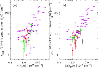
Figure 7.— Integrated optical depths of H₂O-subtracted spectra in the 5.2-6.4 (panel a) and 6.4-7.2 ${\rm\mu m}$ (panel b) ranges plotted against the H₂O ice column densities. The symbol types and colors have the same meaning as in Figs. 5 and 6. Despite the large scatter, it can be concluded that the background stars follow the same correlations as the YSOs (purple asterisks), i.e., the carriers of the absorption are already present in quiescent cloud material.

4.4.4 6.0 $\mu$m band versus $N({\rm H_{2}O})$

Previous work by Keane et al. (2001b) toward massive YSOs, Knez et al. (2005) toward background stars and Boogert et al. (2008) toward low mass YSOs has shown that the 6.0 ${\rm\mu m}$ band can only partly be attributed to solid H₂O. Although H₂O mixed with realistic concentrations of CO₂ fits the long wavelength side (component “C2” in Boogert et al. 2008) better than pure H₂O (Knez et al., 2005; Öberg et al., 2007), it does not explain all absorption. This is the case for the background stars studied here as well. To quantify this, the integrated absorption remaining after subtraction of an amorphous, pure H₂O laboratory ice at $T=$10 K (Hudgins et al., 1993) is plotted against $N{\rm(H_{2}O)}$, showing that the background stars are in line with the YSOs (Fig. 7a; Table 5). The scatter is large, however, which is reflected in a linear correlation coefficient of 0.79. Some of this might be due to uncertainties in $N{\rm(H_{2}O)}$, as many YSOs do not have reliable 3.0 ${\rm\mu m}$ spectra available. Indeed, when only including sources with reliable 3.0 ${\rm\mu m}$ spectra, the correlation coefficient increases to 0.85. Another source of scatter may be the inaccuracy in the continuum determination, especially for the YSOs. Intrinsic abundance variations of the different carriers of the 5.2-6.4 ${\rm\mu m}$ “excess” absorption relative to H₂O must cause some of the scatter as well (Fig. 3).

4.4.5 6.85 $\mu$m band versus $N({\rm H_{2}O})$

The 6.85 ${\rm\mu m}$ band is detected toward many background stars. Its integrated optical depth, calculated after subtracting the long wavelength wing of the H₂O bending mode, is correlated with $N{\rm(H_{2}O)}$ in Fig. 7b, where the YSOs have been plotted as well. As for the 6.0 ${\rm\mu m}$ band, the scatter is large. At a given value of $N{\rm(H_{2}O)}$, the 6.85 ${\rm\mu m}$ band depth varies by a factor of 2. The linear correlation coefficient is 0.88 when including all background stars and YSOs. Within the scatter, there is no systematic difference in the strength of the 6.85 ${\rm\mu m}$ band between YSOs and background stars.

4.4.6 C4/C3 Ratio versus H₂O abundance

The 6.0 and 6.85 ${\rm\mu m}$ bands were decomposed into components C1-C5 in Boogert et al. (2008). It was found that the C4/C3 component ratio varies significantly between YSOs. Sources with large C4/C3 ratios tend to have low H₂O ice abundances (represented by the $N{\rm(H_{2}O)}/\tau{{}_{9.7}}$ ratio) and large degrees of ice crystallization and segregation (Keane et al., 2001b; Boogert et al., 2008), thus indicating that the C4/C3 ratio increases as a result of thermal processing. A similar decomposition was done for the background stars (Fig. 8), and indeed they have low C4/C3 ratios as expected for the cold, unprocessed sight-lines that they trace. Nevertheless, some of the background stars (e.g., toward L328) have low H₂O ice abundances, likely because of the presence of diffuse, ice-free, foreground clouds (§4.4.1) rather than because of the effects of ice sublimation as for YSOs.

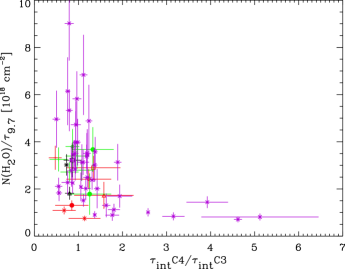
Figure 8.— Ratio of integrated optical depths of the C4 and C3 components (long and short wavelength components of the 6.85 ${\rm\mu m}$ band) plotted versus the H₂O ice column density normalized to the peak optical depth of the 9.7 ${\rm\mu m}$ band (a measure of the H₂O ice abundance). Only values with significance $>2\sigma$ are plotted. Different colors and symbols refer to background stars behind different clouds and cores (see legend of Fig. 5). The values for the YSOs, indicated with purple asterisks, are taken from Boogert et al. (2008). While nearly all sources have C4/C3 ratios near 1, a number of YSOs have significantly larger ratios and at the same time low H₂O abundances.

5. Discussion

5.1. Ice Abundances

The infrared spectra of ices and dust toward background stars presented here provide a baseline for the astrochemical evolution of YSOs. It is shown that the strength and shape of the 3.0, 6.0, 6.85 and 15 ${\rm\mu m}$ ice bands are similar for the quiescent material in isolated cores traced by background stars compared to most previously studied YSOs. Correspondingly, the relative abundances of the ices with secure (CO₂, CH₃OH) and less secure identifications (NH${}^{+}_{4}$) are similar to most YSOs. Species responsible for the 6.0 ${\rm\mu m}$ band, besides H₂O (probably HCOOH, H₂CO, and NH₃), must have abundances similar to YSOs as well. This confirms earlier work on smaller samples (Knez et al., 2005; Bergin et al., 2005), and it firmly establishes that most ices are formed early on in the molecular cloud evolution, and are largely unaltered during the further evolution of the region (e.g., the star formation process) until the YSO thermally processes the ices in the envelope.

The two background stars with the most secure CH₃OH detections (2MASS J18171181-0814012 and 2MASS J18171366-0813188), at $\sim$11% with respect to H₂O, are both located behind the core L429-C. These lines of sight show some of the deepest ice and dust features in the sample, which may have facilitated the detection of the weak 3.53 ${\rm\mu m}$ CH₃OH feature. Indeed, many other background stars in the sample have upper limits or tentative detections at abundances not much less (6-10%) than the detections. Some, e.g. 2MASS J04393886+2611266 in the Taurus Molecular Cloud, have tighter upper limits of 1-3% (Chiar et al. 1996; Table 6), however. Large CH₃OH abundance variations are also observed toward YSOs (Dartois et al., 1999; Pontoppidan et al., 2003b; Boogert et al., 2008).

The presence of solid CH₃OH in quiescent clouds is not unexpected, following theoretical studies (Tielens & Allamandola, 1987; Keane, 2001a), laboratory studies (Watanabe & Kouchi, 2002; Fuchs et al., 2009) and time-dependent (Monte Carlo) simulations (Cuppen et al., 2009). While the laboratory experiments have not yet been fully translated into kinetic parameters, in a general sense, the theoretical studies and kinetic Monte Carlo simulations do show that the CH₃OH/CO ratio is very sensitive to the dust temperature and to the ratio of atomic H to CO in the accreting gas (Keane, 2001a; Cuppen et al., 2009). In this model, an H₂O-rich mantle forms first, because of its higher sublimation temperature, and at $T<$17 K a CO mantle forms on top of that. Accreting H atoms then form H₂CO and CH₃OH. High CH₃OH/CO ratios are indicative of high H/CO ratios of the accreting gas (due to relatively low densities or high local cosmic ray fluxes that destroy H₂). Alternatively, low CH₃OH/CO ratios may reflect relatively elevated dust temperatures ($T>15$ K; Cuppen et al. 2009). Thus local physical conditions are a dominating factor in the formation of CH₃OH, and this may explain the large observed CH₃OH abundance variations in different lines of sight.

5.2. Processing of the Ices

Figure 9.— Profiles of the 3 ${\rm\mu m}$ ice bands observed toward two background stars with the highest (solid and dotted lines), and two background stars with the lowest (dashed and dash-dotted lines) extinctions and peak optical depths in the sample. The spectra are smoothed to a resolving power of 100. The profiles are very similar, indicating a lack of grain growth.

Ice evolution is observed in the envelopes of some YSOs, and it appears that this is mostly due to the effects of heating: apolar CO-rich ices sublimate, and H₂O-rich ices crystallize (Smith et al., 1989; Gerakines et al., 1999; Boogert et al., 2000; Pontoppidan et al., 2008; Boogert et al., 2008). The carrier of the 6.85 ${\rm\mu m}$ band is affected by heating as well: it shifts to longer wavelengths (Keane et al., 2001b; Boogert et al., 2008). Toward background stars, none of these effects are observed. Fig. 8 shows that all background stars with high quality spectra have 6.85 ${\rm\mu m}$ bands peaking at short wavelengths (low C4/C3 ratios). The observed 3.0 ${\rm\mu m}$ bands (Fig. 9) are characteristic of low temperature, amorphous ices. Crystalline ices would peak near 3.1 ${\rm\mu m}$ (Smith et al., 1989).

Finally, an absorption feature in the 5-8 ${\rm\mu m}$ region referred to as C5 in Boogert et al. (2008) (see also Gibb & Whittet 2002), has not been observed toward background stars (Table 5). Although continuum reliability is generally a problem for this shallow feature, detections ($>3\sigma$) were claimed in $\sim$ 30% of the low mass YSOs and $\sim$ 50% of the massive YSOs. The feature could be due to the formation of new molecules by energetic processing of the ices, possibly hydrocarbons (Greenberg et al., 1995) or ions (Schutte & Khanna, 2003). Its absence towards background stars is consistent with an origin in ices processed in the YSO environment, and not by external cosmic rays.

5.3. Ices, Silicates, and the Extinction Curve

Observations show that the properties of dust in diffuse and dense clouds are different. In contrast to diffuse clouds, the mid-infrared extinction in the dense cores studied here ($A_{\rm K}>$1 magn) stays high: at 25 ${\rm\mu m}$ it is still half of that at 2 ${\rm\mu m}$ (Fig. 2b; Chapman et al. 2009; McClure 2009). This is most likely caused by grain growth. Indeed, the calculated $R_{\rm V}$=5.5 (“case B”) extinction curve from Weingartner & Draine (2001) is closer to the observations than their $R_{\rm V}$=3.1 “case A” model (Fig. 2c; Chapman et al. 2009; McClure 2009). Nevertheless, even this extreme case of $R_{\rm V}$=5.5 is systematically too shallow at wavelengths above 5 ${\rm\mu m}$, while the silicate features are too deep. The present work shows that the contribution of ices, which are not included in the Weingartner & Draine (2001) models, to the extinction is not very large: $\sim$25% in the 11-17 ${\rm\mu m}$ wavelength region. Instead, a model with larger grain sizes is needed. Such model would also need to take into account the observed weakness of the 9.7 ${\rm\mu m}$ band of silicates (Figs. 2c and 5a).

Despite the need for larger grains in dense clouds, compared to diffuse clouds, there is no evidence for progressive grain growth in dense clouds for $A_{\rm K}>1$ magn. The empirical extinction curve (Fig. 2) satisfactorily fits most background stars in the sample, for the range of observed $A_{\rm K}$ values of 1.3-6 mag. The same conclusion can be drawn from Fig. 1 in McClure (2009). Also, the 3.0 ${\rm\mu m}$ band profiles are very similar over this $A_{\rm K}$ range (Fig. 9), while a broadening and shift to longer wavelengths would be expected if grain growth occurred. Similarly, the observed linear relation of the 3.0 ${\rm\mu m}$ band with dust column density indicators such as the 9.7 ${\rm\mu m}$ band of silicates and $A_{\rm K}$ (Fig. 5) indicates a lack of progressive grain growth, since larger grains produce 3.0 ${\rm\mu m}$ bands with smaller peak optical depths.

Recent work shows that the silicate band profiles are inconsistent with grain growth beyond 1 ${\rm\mu m}$ (van Breemen et al., 2011), similar to what is found for the 3.0 ${\rm\mu m}$ ice band (Smith et al., 1989). It is thus unlikely that grain growth can fully explain the shallower $A_{\rm K}$ versus $\tau_{9.7}$ relation in the dense medium compared to the diffuse medium (Fig. 5a). Different dust compositions may play a role as well. The silicate bands in dense clouds show a short wavelength wing that could be due to a larger pyroxene/olivine abundance ratio (§4.1). For a more thorough investigation of the $A_{\rm K}$ versus $\tau_{9.7}$ relation one is referred to van Breemen et al. (2011).

6. Conclusions and Future Work

The analysis of 2-25 ${\rm\mu m}$ photometry and spectra of 31 stars tracing the quiescent medium in 16 isolated dense cores yields the following conclusions:

1. An empirical “high resolution” extinction curve derived from one of the background stars confirms extinction curves derived from broad band photometry in high density clouds (Chapman et al., 2009). The curve remains remarkably flat above 10 ${\rm\mu m}$, such that at 25 ${\rm\mu m}$ the extinction is still half that at 2.2 ${\rm\mu m}$. The main caveat is that it is assumed the near-infrared curve is the same as that derived by Indebetouw et al. (2005).

2. The empirical extinction curve, in combination with model spectra of giants, and absorption spectra of H₂O ice and silicates is able to fit the observed data of most background stars well. No systematic deviations are seen as a function of core or $A_{\rm K}$ values (noting that the sample includes only high extinction lines of sight with $A_{\rm K}\gtrsim 1.5$ mag).

3. Model fits of the attenuated stellar continuum are used to isolate the ice and dust absorption features. The 9.7 ${\rm\mu m}$ band of silicates shows a shallower relation with $A_{\rm K}$ compared to the diffuse interstellar medium, thus confirming the results of Chiar et al. (2007) in many more lines of sight. Some background stars, e.g., those behind the L328 core, follow the diffuse medium relation, however.

4. The 3.0 ${\rm\mu m}$ band of H₂O ice is detected in all observed sources. A strong correlation is observed between its peak optical depth and $A_{\rm K}$. Its shape is independent of $A_{\rm K}$, indicating a lack of grain growth at high $A_{\rm K}$ values. This may imply that the shallower relation of $\tau_{9.7}$ with $A_{\rm K}$ in the dense ISM compared to the diffuse ISM is not caused by grain growth. Possibly the dust composition is different, as also suggested by the broader 9.7 ${\rm\mu m}$ band in dense sight-lines (both YSOs and background stars).

5. The 6.0 and 6.85 ${\rm\mu m}$ absorption bands are detected in most background stars. As for YSOs, the 6.0 ${\rm\mu m}$ band is only partially explained by the bending mode of H₂O ice. Additional species, such as HCOOH, H₂CO, CH₃OH, and NH₃ must be responsible for this. Together with the consistent presence of the 6.85 ${\rm\mu m}$ band, which may be due to NH${}_{4}^{+}$, this shows that there is little difference between the ices in quiescent core regions and those surrounding most YSOs. Most ices are apparently formed in the quiescent cloud phase.

6. The discovery of solid CH₃OH in the L-band spectra of several background stars strengthens the previous point. It confirms recent models by Cuppen et al. (2009) that CH₃OH is efficiently formed on the grains in low temperature ($T<15$ K) clouds. Tight upper limits in previously studied sight-lines indicate that the ice composition varies in different environments at the onset of star formation, however. For a proper comparison with the models, observed CH₃OH/CO ratios are needed, i.e., more observations of solid CO toward background stars.

7. Signatures that are assigned to processing of the ices surrounding YSOs, such as profile changes in the 3 ${\rm\mu m}$ ice band, the shifted 6.85 ${\rm\mu m}$ band (i.e., a large C4/C3 ratio) and the presence of the broad C5 components, are not found toward the background stars.

The present work studies ices and the extinction curve in the quiescent medium in isolated dense cores. YSOs in these cores are not well studied. On the other hand, the ices are well studied toward YSOs in large clouds (Taurus, Serpens, Oph, Perseus; Boogert et al. 2008; Pontoppidan et al. 2008; Öberg et al. 2008; Bottinelli et al. 2010), but the background star samples are small (Knez et al., 2005). Thus, future studies will need to compare YSOs and background stars in the same environments to address the origin of the observed variations of the CH₃OH abundance and the strength of the 6.0 and 6.8 ${\rm\mu m}$ ice bands (Figs. 3 and 7). Furthermore, while there is now much observational evidence that the dust properties in the dense and diffuse medium are quite different, the cause of this is not understood, warranting further theoretical and perhaps laboratory investigations.

References

- Allamandola et al. (1992) Allamandola, L. J., Sandford, S. A., Tielens, A. G. G. M., & Herbst, T. M. 1992, ApJ, 399, 134
- Beichman et al. (1986) Beichman, C. A., Myers, P. C., Emerson, J. P., Harris, S., Mathieu, R., Benson, P. J., & Jennings, R. E. 1986, ApJ, 307, 337
- Bergin et al. (2005) Bergin, E. A., Melnick, G. J., Gerakines, P. A., Neufeld, D. A., & Whittet, D. C. B. 2005, ApJ, 627, L33
- Bernstein et al. (2002) Bernstein, M. P., Dworkin, J. P., Sandford, S. A., Cooper, G. W., & Allamandola, L. J. 2002, Nature, 416, 401
- Bohlin et al. (1978) Bohlin, R. C., Savage, B. D., & Drake, J. F. 1978, ApJ, 224, 132
- Bohren & Huffman (1983) Bohren, C. F., & Huffman, D. R. 1983, Absorption and Scattering of Light by Small Particles (New York: John Wiley & Sons)
- Boogert et al. (1997) Boogert, A. C. A., Schutte, W. A., Helmich, F. P., Tielens, A. G. G. M., & Wooden, D. H. 1997, A&A, 317, 929
- Boogert et al. (2000) Boogert, A. C. A., et al. 2000, A&A, 353, 349
- Boogert et al. (2002) Boogert, A. C. A., Blake, G. A., & Tielens, A. G. G. M. 2002, ApJ, 577, 271
- Boogert & Ehrenfreund (2004) Boogert, A. C. A., & Ehrenfreund, P. 2004, Astrophysics of Dust, 309, 547
- Boogert et al. (2008) Boogert, A. C. A., et al. 2008, ApJ, 678, 985
- Bottinelli et al. (2010) Bottinelli, S., et al. 2010, ApJ, 718, 1100
- Brooke et al. (1996) Brooke, T. Y., Sellgren, K., & Smith, R. G. 1996, ApJ, 459, 209
- Chapman et al. (2009) Chapman, N. L., Mundy, L. G., Lai, S.-P., & Evans, N. J. 2009, ApJ, 690, 496
- Chiar et al. (1995) Chiar, J. E., Adamson, A. J., Kerr, T. H., & Whittet, D. C. B. 1995, ApJ, 455, 234
- Chiar et al. (1996) Chiar, J. E., Adamson, A. J., & Whittet, D. C. B. 1996, ApJ, 472, 665
- Chiar et al. (2007) Chiar, J. E., et al. 2007, ApJ, 666, L73
- Chiar et al. (2011) Chiar, J. E., et al. 2011, ApJ(submitted)
- Cuppen et al. (2009) Cuppen, H. M., van Dishoeck, E. F., Herbst, E., & Tielens, A. G. G. M. 2009, A&A, 508, 275
- Dartois et al. (1999) Dartois, E., Schutte, W., Geballe, T. R., Demyk, K., Ehrenfreund, P., & d’Hendecourt, L. 1999, A&A, 342, L32
- Dartois & d’Hendecourt (2001) Dartois, E., & d’Hendecourt, L. 2001, A&A, 365, 144
- Decin et al. (2004) Decin, L., Morris, P. W., Appleton, P. N., Charmandaris, V., Armus, L., & Houck, J. R. 2004, ApJS, 154, 408
- Dorschner et al. (1995) Dorschner, J., Begemann, B., Henning, T., Jaeger, C., & Mutschke, H. 1995, A&A, 300, 503
- Evans (1999) Evans, N. J., II 1999, ARA&A, 37, 311
- Evans et al. (2003) Evans, N. J., II, et al. 2003, PASP, 115, 965
- Evans et al. (2007) Evans, N. J., II, et al. 2007, Final Delivery of Data from the c2d Legacy Project: IRAC and MIPS (Pasadena: SSC), http://ssc.spitzer.caltech.edu/legacy/
- Fuchs et al. (2009) Fuchs, G. W., Cuppen, H. M., Ioppolo, S., Romanzin, C., Bisschop, S. E., Andersson, S., van Dishoeck, E. F., & Linnartz, H. 2009, A&A, 505, 629
- Gerakines et al. (1995) Gerakines, P. A., Schutte, W. A., Greenberg, J. M., & van Dishoeck, E. F. 1995, A&A, 296, 810
- Gerakines et al. (1999) Gerakines, P. A., et al. 1999, ApJ, 522, 357
- Gibb & Whittet (2002) Gibb, E. L., & Whittet, D. C. B. 2002, ApJ, 566, L113
- Gibb et al. (2004) Gibb, E. L., Whittet, D. C. B., Boogert, A. C. A., & Tielens, A. G. G. M. 2004, ApJS, 151, 35
- Greenberg et al. (1995) Greenberg, J. M., Li, A., Mendoza-Gomez, C. X., Schutte, W. A., Gerakines, P. A., & de Groot, M. 1995, ApJ, 455, L177
- Hagen et al. (1981) Hagen, W., Tielens, A. G. G. M., & Greenberg, J. M. 1981, Chem. Phys., 56, 367
- Hudgins et al. (1993) Hudgins, D. M., Sandford, S. A., Allamandola, L. J., & Tielens, A. G. G. M. 1993, ApJS, 86, 713
- Indebetouw et al. (2005) Indebetouw, R., et al. 2005, ApJ, 619, 931
- Kane & Sahu (2003) Kane, S. R., & Sahu, K. C. 2003, ApJ, 582, 743
- Keane (2001a) Keane, J. V. 2001a, Ph.D. Thesis, Chapter 7
- Keane et al. (2001b) Keane, J. V., Tielens, A. G. G. M., Boogert, A. C. A., Schutte, W. A., & Whittet, D. C. B. 2001b, A&A, 376, 254
- Kemper et al. (2004) Kemper, F., Vriend, W. J., & Tielens, A. G. G. M. 2004, ApJ, 609, 826
- Kerkhof et al. (1999) Kerkhof, O., Schutte, W. A., & Ehrenfreund, P. 1999, A&A, 346, 990
- Knez et al. (2005) Knez, C., et al. 2005, ApJ, 635, L145
- Lada et al. (1999) Lada, C. J., Alves, J., & Lada, E. A. 1999, The Physics and Chemistry of the Interstellar Medium, 161
- McClure (2009) McClure, M. 2009, ApJ, 693, L81
- McLean et al. (1998) McLean, I. S., et al. 1998, Proc. SPIE, 3354, 566
- Myers & Benson (1983) Myers, P. C., & Benson, P. J. 1983, ApJ, 266, 309
- Öberg et al. (2007) Öberg, K. I., Fraser, H. J., Boogert, A. C. A., Bisschop, S. E., Fuchs, G. W., van Dishoeck, E. F., & Linnartz, H. 2007, A&A, 462, 1187
- Öberg et al. (2008) Öberg, K. I., Boogert, A. C. A., Pontoppidan, K. M., Blake, G. A., Evans, N. J., Lahuis, F., & van Dishoeck, E. F. 2008, ApJ, 678, 1032
- Pontoppidan et al. (2003a) Pontoppidan, K. M., et al. 2003a, A&A, 408, 981
- Pontoppidan et al. (2003b) Pontoppidan, K. M., Dartois, E., van Dishoeck, E. F., Thi, W.-F., & d’Hendecourt, L. 2003b, A&A, 404, L17
- Pontoppidan et al. (2008) Pontoppidan, K. M., et al. 2008, ApJ, 678, 1005
- Reach et al. (2009) Reach, W. T., et al. 2009, ApJ, 690, 683
- Roche & Aitken (1984) Roche, P. F., & Aitken, D. K. 1984, MNRAS, 208, 481
- Schutte et al. (1993) Schutte, W. A., Allamandola, L. J., & Sandford, S. A. 1993, Icarus, 104, 118
- Schutte et al. (1999) Schutte, W. A., et al. 1999, A&A, 343, 966
- Schutte & Khanna (2003) Schutte, W. A., & Khanna, R. K. 2003, A&A, 398, 1049
- Shu et al. (1987) Shu, F. H., Adams, F. C., & Lizano, S. 1987, ARA&A, 25, 23
- Skrutskie et al. (2006) Skrutskie, M. F., et al. 2006, AJ, 131, 1163
- Smith et al. (1989) Smith, R. G., Sellgren, K., & Tokunaga, A. T. 1989, ApJ, 344, 413
- Tanaka et al. (1990) Tanaka, M., Sato, S., Nagata, T., & Yamamoto, T. 1990, ApJ, 352, 724
- Tielens & Hagen (1982) Tielens, A. G. G. M., & Hagen, W. 1982, A&A, 114, 245
- Tielens & Allamandola (1987) Tielens, A. G. G. M., & Allamandola, L. J. 1987, Interstellar Processes, 134, 397
- Tielens et al. (1991) Tielens, A. G. G. M., Tokunaga, A. T., Geballe, T. R., & Baas, F. 1991, ApJ, 381, 181
- van Breemen et al. (2011) van Breemen, J. M., et al. 2011, A&A(in press)
- Watanabe & Kouchi (2002) Watanabe, N., & Kouchi, A. 2002, ApJ, 571, L173
- Weingartner & Draine (2001) Weingartner, J. C., & Draine, B. T. 2001, ApJ, 548, 296
- Whittet et al. (1983) Whittet, D. C. B., Bode, M. F., Baines, D. W. T., Longmore, A. J., & Evans, A. 1983, Nature, 303, 218
- Whittet et al. (1998) Whittet, D. C. B., et al. 1998, ApJ, 498, L159
- Whittet et al. (2001) Whittet, D. C. B., Pendleton, Y. J., Gibb, E. L., Boogert, A. C. A., Chiar, J. E., & Nummelin, A. 2001, ApJ, 550, 793
- Whittet (2003) Whittet, D. C. B. 2003, Dust in the galactic environment, 2nd ed. by D.C.B. Whittet. Bristol: Institute of Physics (IOP) Publishing, 2003 Series in Astronomy and Astrophysics, ISBN 0750306246.,
- Whittet et al. (2009) Whittet, D. C. B., Cook, A. M., Chiar, J. E., Pendleton, Y. J., Shenoy, S. S., & Gerakines, P. A. 2009, ApJ, 695, 94
- Young et al. (2004) Young, C. H., et al. 2004, ApJS, 154, 396
- Zasowski et al. (2009) Zasowski, G., Kemper, F., Watson, D. M., Furlan, E., Bohac, C. J., Hull, C., & Green, J. D. 2009, ApJ, 694, 459