Embedded Eigenvalues and the Nonlinear Schrödinger Equation

Abstract.

A common challenge to proving asymptotic stability of solitary waves is understanding the spectrum of the operator associated with the linearized flow. The existence of eigenvalues can inhibit the dispersive estimates key to proving stability. Following the work of Marzuola & Simpson, we prove the absence of embedded eigenvalues for a collection of nonlinear Schrödinger equations, including some one and three dimensional supercritical equations, and the three dimensional cubic-quintic equation. Our results also rule out nonzero eigenvalues within the spectral gap and, in 3D, endpoint resonances.

The proof is computer assisted as it depends on the sign of certain inner products which do not readily admit analytic representations. Our source code is available for verification at http://www.math.toronto.edu/simpson/files/spec_prop_asad_simpson_code.zip.

1. Introduction

The nonlinear Schrödinger equation (NLS) in $\mathbb{R}^{d+1}$ dimensions,

(1.1) $$i\psi_{t}+\nabla^{2}\psi+f(|\psi|^{2})\psi=0,\quad\psi(0,\mathbf{x})=\psi_{0}(\mathbf{x}),$$

appears as a leading order approximation to a wide variety of natural and engineered systems, including optics, plasma physics, and fluid mechanics. It is also a model equation for the studying the competition between nonlinear and dispersive effects. See Sulem & Sulem, [21], for details and examples.

1.1. Solitons

For appropriate choices of the nonlinearity, $f:\mathbb{R}\to\mathbb{R}$, the equation will possess solitary wave solutions, smooth localized solutions of (1.1) satisfying the ansatz

(1.2) $$\psi(t,\mathbf{x})=e^{i\omega t}R(\mathbf{x};\omega),\quad\omega>0.$$

$R$ then solves the nonlinear elliptic equation

(1.3) $$-\omega R+\nabla^{2}R+f(\lvert R\rvert^{2})R=0.$$

The solutions are assumed to have finite $L^{2}$ norm and vanish at infinity.

These nonlinear bound states, deemed solitary waves or solitons, are of interest both as mathematical objects and in applications. This raises the question of whether or not these solutions are stable to the flow of (1.1). Developing tools for assessing stability is the main purpose of this paper.

1.2. Stability

With regard to solitary waves, the two types of stability typically discussed are orbital stability and asymptotic stability. Orbital stability, alternatively called Lyapunov or modulational stability, asserts that if the data is close to a solitary wave, it remains close, modulo a group of symmetries associated with the equation.

In [22, 23], M.I. Weinstein proved that orbital stability of a solution to (1.3) could be assessed by computing the sign of

(1.4) $$\frac{d}{d\omega}\int\lvert R({\bf x};\omega)\rvert^{2}d{\bf x}.$$

When it is positive, the solitons are stable; when it is negative, they are unstable. This work was subsequently generalized for Hamiltonian equations by Grillakis, Shatah, & Strauss [9, 10].

For NLS with a power, or monomial, nonlinearity of the form $f(s)=s^{\sigma}$, the transition between stable and unstable solitons is determined by the product $\sigma d$. If $\sigma d<2$, the solitary waves are stable, otherwise they are unstable. These regimes, $\sigma d<2,=2,>2$ correspond to the subcritical, critical, and supercritical forms of (1.1), and are intimately related to the well-posedness of NLS, [21].

Of course, orbital stability does not tell us of the limiting behavior of the solution. An orbitally stable soliton could perpetually oscillate through the symmetry group of the equation. It is our expectation that perturbations of stable solitons diminish as $t\to\infty$, and the solution relaxes to a particular solitary wave with a fixed set of parameters. We turn to asymptotic stability to understand the dynamics as $t\to\infty$.

Asymptotic stability is usually proven by expanding (1.1) about the solitary wave solution, $\psi=e^{i\omega t}(R(\cdot;\omega)+u+iv)$ to arrive at an equation for the perturbation, $p=u+iv$,

(1.5) $$\begin{split}\partial_{t}\begin{pmatrix}u\\ v\end{pmatrix}&=JL\begin{pmatrix}u\\ v\end{pmatrix}+{\bf F}(u,v)\\ &=\begin{pmatrix}0&1\\ -1&0\end{pmatrix}\begin{pmatrix}L_{+}&0\\ 0&L_{-}\end{pmatrix}\begin{pmatrix}u\\ v\end{pmatrix}+{\bf F}.\end{split}$$

${\bf F}$ contains terms that are nonlinear in the perturbation, and the scalar operators $L_{\pm}$ are given by

(1.6a) $$L_{+} =-\nabla^{2}+\omega-f(R^{2})-2f^{\prime}(R^{2})R^{2}=-\nabla^{2}+\omega+V_{+},$$

(1.6b) $$L_{-} =-\nabla^{2}+\omega-f(R^{2})=-\nabla^{2}+\omega+V_{-}.$$

Proving asymptotic stability of the solitary wave will require Strichartz estimates of the form

(1.7) $$\lVert e^{JLt}f\rVert_{L^{p}_{t}L^{q}_{x}}\lesssim\lVert f\rVert_{L^{r}_{x}}.$$

With such an estimate, one can conclude linear stability of the soliton from the temporal decay of a solution to the linear problem

$${\bf p}_{t}=JL{\bf p},\quad{\bf p}=(u,v)^{T}.$$

This decay can then be used to show that the nonlinear part of the flow, ${\bf F}$ in (1.5), is dominated by the linear part can can be treated perturbatively. Successful implementations include Buslaev & Perelman, [1], Buslaev & Sulem, [2], Cuccagna and Rodnianski, Soffer & Schlag, [3, 15] and more recently to Schlag and Krieger & Schlag, [11, 16]. These last two works, where the authors show the asymptotic stability of a constrained soliton which is orbitally unstable, are closely related to the present results.

1.3. The Spectrum & Embedded Eigenvalues

Estimates of the form (1.7) require adequate knowledge of the spectrum of $JL$, $\sigma(JL)$. Since the solitons are highly localized, $JL$ is easily shown to be a relatively compact perturbation of

(1.8) $$\begin{pmatrix}0&-\nabla^{2}+\omega\\ \nabla^{2}-\omega&0\end{pmatrix}$$

which has as its essential spectrum

$$(-i\infty,-i\omega]\cup[i\omega,i\infty)$$

This can easily be computed by the Fourier transform. Thus

(1.9) $$\sigma_{\mathrm{ess}}(JL)=i(-\infty,-\omega]\cup i[\omega,\infty)\subseteq\sigma(JL)$$

See [7] for additional details. By direct computations, one can show that the origin is an eigenvalue of $JL$ of algebraic multiplicity at least $2d+2$. See section 2.1 below for the elements of the kernel, and Figure 1 for a visualization of the spectrum of the problems considered here.

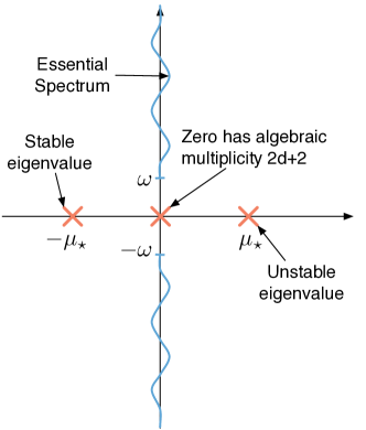
Figure 1. The generic spectrum of $JL$ for an orbitally unstable soliton. The instability is due to the positive eigenvalue, $\mu_{\star}$.

The existence of purely imaginary eigenvalues both within the spectral gap, $[-i\omega,i\omega]$, and embedded in the essential spectrum and resonances can obstruct the Strichartz estimates. Many results on asymptotic stability of NLS solitons, including [2, 7, 16], have explicitly assumed:

1. $JL$ has no embedded eigenvalues;

2. The only eigenvalue within the spectral gap is zero;

3. The endpoints of the essential spectrum, $\pm i\omega$, are not resonances.

We are thus motivated to find ways of rigorously proving these assumptions.

Some previous results on these spectral questions were addressed by Krieger & Schlag in 1D for $f(s)=s^{\sigma}$ with $\sigma>4$ (supercritical), [11]. Alternatively, Cuccagna & Pelinovksy and Cuccagna, Pelinovsky, & Vougalter [4, 5] showed that in 1D, embedded eigenvalues with positive Krein signature can exist and not disrupt asymptotic stability. But an extension of their approach, based on the Fermi Golden Rule, to higher dimensions remains a challenge; it may be easier to prove that such states are absent. In [6], Demanet & Schlag gave a numerically assisted proof for the absence of non zero eigenvalues within the spectral gap for 3D NLS with a power nonlinearity with

(1.10) $$0.913958905\pm 10^{−8}<\sigma\leq 1$$

More recently, Marzuola & Simpson, [12], proved that the 3D cubic problem has no purely imaginary eigenvalues or endpoint resonances. This proof required a modest amount of numerical assistance to compute:

• The dimension of the negative subspace of several 1D Schrödinger operators;

• The inner products of solutions of several 1D boundary value problems.

In this work, we apply the approach of [12], to some other equations.

1.4. Main Results

Our main results are for the 1D and 3D supercritical NLS equations with $f(s)=s^{\sigma}$, and the 3D cubic-quintic nonlinear Schrödinger equation (CQNLS) and for the 1D supercritical NLS,

(1.11) $$i\psi_{t}+\nabla^{2}\psi+(\lvert\psi\rvert^{2}-\gamma\lvert\psi\rvert^{4})\psi=0.$$

Theorem 1.

For 3D NLS with

(1.12) $$0.807425<\sigma<1.12092$$

$JL$, the linearization about the soliton $R=R(\cdot;1)$, has no purely imaginary eigenvalues or endpoint resonances.

Theorem 2.

For 3D CQNLS with

(1.13) $$\gamma<0.00989115$$

$JL$, the linearization about the soliton $R=R(\cdot;1)$, has no purely imaginary eigenvalues or endpoint resonances.

For the sake of exploring the limits of our approach, we also prove:

Theorem 3.

For 1D NLS with

(1.14) $$2.4537956056<\sigma<6.1288520139$$

$JL$, the linearization about the soliton $R=R(\cdot;1)$, has no purely imaginary eigenvalues.

As previously mentioned, Theorem 3 has been rigorously established for all $\sigma>2$, [11].

To prove these theorems, we first show that a particular bilinear form, which would vanish at any purely imaginary eigenvalue or endpoint resonance, is coercive on an appropriate subspace. This coercivity allows us to immediately rule out such states. To proceed we must define distorted variants of $L_{\pm}$ which form the bilinear form.

Definition 1.1.

Given $L_{\pm}$ and a skew adjoint operator $\Lambda$, define the two Schrödinger operators via the commutator relations:

(1.15) $$\mathcal{L}_{\pm}=\frac{1}{2}[L_{\pm},\Lambda]=-\nabla^{2}+\mathcal{V}_{\pm}.$$

For ${\bf z}=(u,v)^{T}\in L^{2}\times L^{2}$, define the bilinear form

(1.16) $$\begin{split}{\mathcal{B}}({\bf z},{\bf z})&={\mathcal{B}}_{+}(u,u)+{\mathcal{B}}_{-}(v,v)\\ &=\left\langle\mathcal{L}_{+}u,u\right\rangle+\left\langle\mathcal{L}_{-}v,v\right\rangle\end{split}$$

The operator $JL$ is said to satisfy the spectral property on the subspace $\mathcal{U}\subseteq L^{2}\times L^{2}$ if

(1.17) $${\mathcal{B}}({\bf z},{\bf z})\gtrsim\int\left(\lvert\nabla{\bf z}\rvert^{2}+e^{-\lvert\bf x\rvert}\lvert{\bf z}\rvert^{2}\right)d{\bf x}$$

The skew adjoint operator $\Lambda$ and the subspace $\mathcal{U}$ are, at this point, unspecified. In our work, we use

(1.18) $$\Lambda=\frac{d}{2}+{\bf x}\cdot\nabla.$$

The potentials, $\mathcal{V}_{\pm}$, this induces from $L_{\pm}$ are

(1.19a) $$\mathcal{V}_{+} =\tfrac{1}{2}{\bf x}\cdot\nabla\left[f(R^{2})+2f^{\prime}(R^{2})R^{2}\right]=r(3f^{\prime}(R^{2})+2f^{\prime\prime}(R^{2})R^{2})RR^{\prime}$$

(1.19b) $$\mathcal{V}_{-} =\tfrac{1}{2}{\bf x}\cdot\nabla\left[f(R^{2})\right]=rf^{\prime}(R^{2})RR^{\prime}$$

For the 3D problems we consider, these correspond to:

$$f(s)=s^{\sigma}: \mathcal{V}_{+}=\sigma(2\sigma+1)R^{2\sigma-1}R^{\prime},\quad\mathcal{V}_{-}=\sigma rR^{2\sigma-1}R^{\prime}$$

$$f(s)=s-\gamma s^{2}: \mathcal{V}_{+}=r(3R-10\gamma R^{3})R^{\prime},\quad\mathcal{V}_{-}=r(R-2\gamma R^{3})R^{\prime}$$

The particulars of this subspace will be discussed in Section 2.2. This Spectral Property appeared in the works of Merle & Raphaël, and Fibich, Merle & Raphaël in their proofs of the $\log-\log$ blowup of $L^{2}$ critical NLS, [8, 13]. It has similarly appeared in Simpson & Zwiers, in a proof of the $\log-\log$ blow up for vortex solitons in 2D cubic NLS, [20]

The role of this Spectral Property was identified by G. Perelman, [14], and leads directly to:

Theorem 4.

If the Spectral Property holds for $JL$, then $JL$ has no imaginary eigenvalues on $\mathcal{U}$.

The proof is quite simple and appears in [12]. Briefly, one shows by direct computation that $\mathcal{B}$ vanishes at any eigenstates corresponding to imaginary eigenvalues. In 3D, this same analysis will rule out endpoint resonances.

Though all of the cases for which we have results correspond to orbitally unstable solitons, the results remain of interest. They can be used to prove results on constrained asymptotic stability, as in [16], where one projects away from the linearly unstable direction of $JL$. In addition they are intrinsically interesting as results on the spectrum of Hamiltonian operators. Finally, these theorems also map out the scope of success for this approach.

Our paper is organized as follows. In Section 2 we review some relevant algebraic properties of $JL$, and define the subspace, $\mathcal{U}$, that will be used to prove the Spectral Property. In Section 3, we present some preliminary results used in the proof. Section4 presents our computations and the main results. Some discussion of the limits of this approach are raised in Section 5.

Acknowledgements: The authors wish to thank J.L. Marzuola for some helpful comments, D.E. Pelinovsky for suggesting a comparison with the Demanet & Schlag threshold, and C. Sulem for suggesting the extension to CQNLS. This work was supported in part by NSERC.

2. Algebraic Structure

As noted in the introduction, $\sigma(JL)$ includes the essential spectrum, lying on a portion of the imaginary axis, along with some eigenvalues. Since the algebraic structure of $JL$ is used in our proof, we review the discrete spectrum here.

2.1. Discrete Spectrum

Given that (1.1) supports a solitary wave solution, we readily observe:

Theorem 5 (Kernel).

$JL$ has a kernel of algebraic multiplicity at least $2d+2$:

$$JL\begin{pmatrix}0\\ R\end{pmatrix}=0,\quad JL\begin{pmatrix}\partial_{x_{j}}R\\ 0\end{pmatrix}=0$$

$$JL\begin{pmatrix}\partial_{\omega}R\\ 0\end{pmatrix}=-\begin{pmatrix}0\\ R\end{pmatrix}\quad JL\begin{pmatrix}0\\ x_{j}R\end{pmatrix}=-2\begin{pmatrix}\partial_{x_{j}}R\\ 0\end{pmatrix}$$

for $j=1,\ldots d$.

For power nonlinearities, we can, and do, use, that

(2.1) $$2\partial_{\omega}|_{\omega=1}R=\tfrac{1}{\sigma}R+{\bf x}\cdot\nabla R.$$

In addition to these elements, there are two additional eigenstates that can reside on the imaginary axis, the origin, or the real axis, depending on the slope condition, (1.4). For orbitally unstable problems we have:

Theorem 6 (Off Axis Eigenvalues).

There exists a pair of real, nonzero, eigenvalues located at $\pm\mu_{\star}$. Corresponding to $\mu_{\star}>0$, is the eigenstate $\boldsymbol{\phi}=(\phi_{1},\phi_{2})^{T}$. For $d=1$, the $\phi_{j}$ are even functions, and for $d>1$, the $\phi_{j}$ are radially symmetric.

These off axis eigenvalues appear in Figure 1. Their existence follows form the results of [9]. Alternatively, Schlag presented a continuity argument in [16] that relies on the knowledge of the two additional eigenstates that appear at the origin in the critical case, $\sigma d=2$.

It is well known that for $f(s)=s^{\sigma}$, the slope is negative when $\sigma d>2$. Due to scaling, this holds for all $\omega>0$. For CQNLS, some solitons are stable and others are unstable, depending on $\gamma$ and the soliton parameter $\omega$. In this work, we shall fix $\omega=1$ for which solitons are known to exist provided $\gamma<3/16$, [21]. We now determine the range of $0\leq\gamma<3/16$ for which the solitons are unstable.

At $\gamma=0$, this corresponds to the 3D cubic problem, which we know to be unstable. By continuity, we expect there is some open set of $\gamma$ near zero for which the solitons are orbitally unstable. To identify the threshold value of $\gamma$, we numerically compute (1.4), and find that it changes sign at

(2.2) $$\gamma_{\star}\approx 0.0255453.$$

The slope condition values as a function of $\gamma$ are plotted in Figure 2. See Appendix A for details of this computation.

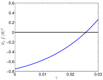
Figure 2. The numerically computed (1.4) at $\omega=1$ changes from negative to positive at the critical $\gamma_{\star}\approx 0.0255453$.

2.2. Subspaces

As discussed in Section 2.2 of [12], the subspace $\mathcal{U}$ for which we wish to establish the Spectral Property of Definition 1.1 must satisfy two properties:

• If they exist, eigenstates of purely imaginary eigenvalues must reside in $\mathcal{U}$;

• $\mathcal{U}$ must be orthogonal to the negative subspaces of ${\mathcal{L}}_{\pm}$.

Obviously, if both properties are satisfied, then there are no purely imaginary eigenvalues. But it may be possible to construct a $\mathcal{U}$ that is orthogonal to the eigenstates of such eigenvalues, and on which the operators are positive.

A practical subspace makes use of the eigenstates of the adjoint operator, $(JL)^{\ast}$. These are closely related to the elements of $JL$. Given $\boldsymbol{\psi}=(\psi_{1},\psi_{2})^{T}$, an eigenstate of $JL$ with eigenvalue $\lambda$,

(2.3) $$(JL)^{\ast}\begin{pmatrix}\psi_{2}\\ \psi_{1}\end{pmatrix}=-\lambda\begin{pmatrix}\psi_{2}\\ \psi_{1}\end{pmatrix}$$

Consequently,

Proposition 2.1.

Let $\boldsymbol{\psi}=(\psi_{1},\psi_{2})^{T}$ be an eigenstate corresponding to a purely imaginary eigenvalue of $JL$.

• Any element of $\ker_{g}((JL)^{\ast})$ is orthogonal to $\boldsymbol{\psi}$;

• The unstable eigenstate $\boldsymbol{\phi}$ of $JL$ satisfies the relations:

  $$\left\langle\psi_{1},\phi_{2}\right\rangle=0,\quad\left\langle\psi_{2},\phi_{1}\right\rangle=0.$$

See Section 2.2 of [12] for a proof. Using this, we define $\mathcal{U}$ to be the orthogonal complement of

(2.4) $${\mathrm{span}}\left\{\begin{pmatrix}R\\ 0\end{pmatrix},\begin{pmatrix}0\\ \partial_{\omega}R\end{pmatrix},\begin{pmatrix}0\\ \partial_{x_{j}}R\end{pmatrix},\begin{pmatrix}{x_{j}}R\\ 0\end{pmatrix},\begin{pmatrix}\phi_{2}\\ 0\end{pmatrix},\begin{pmatrix}0\\ \phi_{1}\end{pmatrix}\right\}$$

Indeed,

Theorem 7.

If the Spectral Property can be established on $\mathcal{U}$ given by the orthogonal complement to (2.4), or any subspace containing $\mathcal{U}$, $JL$ will not have any purely imaginary eigenvalues on $L^{2}\times L^{2}$.

We succeed in proving:

Theorem 8.

Assume ${\bf z}=(f,g)^{T}\in L^{2}\times L^{2}$ satisfies the orthogonality conditions

(2.5) $$\left\langle f,R\right\rangle=\left\langle f,\phi_{2}\right\rangle=\left\langle g,\partial_{\omega}|_{\omega=1}R\right\rangle=\left\langle g,\phi_{1}\right\rangle=\left\langle f,{\bf x}R\right\rangle=0$$

Then the Spectral Property holds for:

3D NLS:

Provided

$$0.807425<\sigma<1.12092;$$

3D CQNLS:

Provided

$$\gamma<0.00989115;$$

1D NLS:

Provided

$$2.4537956056<\sigma<6.1288520139.$$

For 1D and 3D NLS with power nonlinearities, we use (2.1).

3. Preliminaries

We shall prove the coercivity of $\mathcal{B}$ in three steps, closely following [8, 12], and omitting some details.

• In 1D, we decompose into even and odd functions and study

  (3.1) $$\begin{split}{\mathcal{B}}_{+}(f,f)+{\mathcal{B}}_{-}(g,g)&={\mathcal{B}}_{+}^{(e)}(f^{(e)},f^{(e)})+{\mathcal{B}}_{+}^{(o)}(f^{(o)},f^{(o)})\\ &\quad+{\mathcal{B}}_{-}^{(e)}(g^{(e)},g^{(e)})+{\mathcal{B}}_{-}^{(o)}(g^{(o)},g^{(o)})\end{split}$$

  We then show that on $\mathcal{U}$, each of the four forms, ${\mathcal{B}}_{\pm}^{(e/o)}$, is positive.

  Similarly, in 3D, we decompose into spherical harmonics,

  (3.2) $$\begin{split}{\mathcal{B}}_{+}(f,f)+{\mathcal{B}}_{-}(g,g)&=\sum_{k=0}^{\infty}\sum_{l=0}^{L_{k}}{\mathcal{B}}_{+}^{(k)}(f^{(k,l)},f^{(k,l)})\\ &\quad+\sum_{k=0}^{\infty}\sum_{l=0}^{L_{k}}{\mathcal{B}}_{-}^{(k)}(g^{(k,l)},g^{(k,l)})\end{split}$$

  where $f^{(k,l)}$ and $g^{(k,l)}$ are the components of $f$ and $g$ in harmonic $k$ with angular component $l$. As ${\mathcal{L}}_{\pm}$ are radially symmetric operators, they are independent of $l$. Here too, we shall prove positivity of each ${\mathcal{B}}_{\pm}^{(k)}$ on $\mathcal{U}$.

• For each of these bilinear forms, we shall determine the codimension of a subspace on which they are positive, called its index. This is problem specific and can vary with the dimension and choice of nonlinearity.

• Lastly, we shall show that the $L^{2}$ orthogonality of $f$ and $g$ to $\mathcal{U}^{\perp}$ induces orthogonality, with respect to to the bilinear form, to the negative subspaces of the form. See Section 4.1.3 for an example.

3.1. Indexes and Eigenvalues

The index of a bilinear form $B$ on a vector space $V$ is defined as

(3.3) $$\begin{split}{\mathrm{ind}}_{V}(B)\equiv\max\{k\in\mathbb{N}\mid&\text{there exists a subspace $\tilde{V}\subseteq V$}\\ &\text{of codimension $k$ such that $B|_{\tilde{V}}$ is positive}\}\end{split}$$

To compute the indexes, we rely on the following propositions:

Proposition 3.1.

Let $U^{(e)}$ and $U^{(o)}$ solve the initial value problems

$$LU^{(e)} =-\frac{d^{2}}{dx^{2}}u^{(e)}+V(x)U^{(e)}=0,\quad U^{(e)}(0)=1,\quad\frac{d}{dx}U^{(e)}(0)=0$$

$$LU^{(o)} =-\frac{d^{2}}{dx^{2}}u^{(o)}+V(x)U^{(o)}=0,\quad U^{(o)}(0)=0,\quad\frac{d}{dx}U^{(o)}(0)=1$$

where $V$ is even, sufficiently smooth, and $\lvert V(x)\rvert\lesssim e^{-\kappa\lvert x\rvert}$, $\kappa>0$, and let

$$B(\cdot,\cdot)\equiv\left\langle L\cdot,\cdot\right\rangle.$$

Then the number of zeros of $U^{(e)}$ and $U^{(o)}$ is finite, and

$${\mathrm{ind}}_{H^{1}_{e}}(B) =\text{number of positive roots of $U^{(e)}$}$$

$$=\text{number of negative eigenvalues in $H^{1}_{e}$}$$

$${\mathrm{ind}}_{H^{1}_{o}}(B) =\text{number of positive roots of $U^{(o)}$}$$

$$=\text{number of negative eigenvalues in $H^{1}_{o}$}$$

$H^{1}_{e}$ and $H^{1}_{o}$ are the even and odd subspaces of $H^{1}$.

Proposition 3.2.

Let $U^{(k)}$ solve the initial value problem

$$L^{(k)}U^{(k)}=\left[-\frac{d^{2}}{dr^{2}}-\frac{2}{r}\frac{d}{dr}+V(r)+\frac{k^{2}}{r^{2}}\right]U^{(k)}=0$$

$$\lim_{r\to 0}r^{-k}U^{(k)}(r)=1,\quad\lim_{r\to 0}\frac{d}{dr}\left(r^{-k}U^{(k)}(r)\right)=0,$$

for $k=0,1,2,3,\ldots$ where $V$ is sufficiently smooth, and $\lvert V(r)\rvert\lesssim e^{-\kappa\lvert r\rvert}$,$\kappa>0$, and let

$$B^{(k)}(\cdot,\cdot)\equiv\left\langle L^{(k)}\cdot,\cdot\right\rangle.$$

Then the number of zeros of $U^{(k)}$ is finite, and

$${\mathrm{ind}}_{H^{1}_{{\mathrm{rad}}}}(B^{(0)}) =\text{number of positive roots of $U^{(0)}$}$$

$$=\text{number of negative eigenvalues in $H^{1}_{\mathrm{rad}}$}$$

$${\mathrm{ind}}_{H^{1}_{{\mathrm{rad}}+}}(B^{(k)}) =\text{number of positive roots of $U^{(k)}$, for $k=1,2,\ldots$}$$

$$=\text{number of negative eigenvalues in $H^{1}_{{\mathrm{rad}}+}$}$$

The space $H^{1}_{{\mathrm{rad}}+}$ is the subspace of radially symmetric $H^{1}$ functions for which

$$\int\lvert f\rvert^{2}\lvert{\bf x}\rvert^{-2}d{\bf x}<\infty.$$

The indexes in the different harmonics have an invaluable monotonicity property that permits us to restrict our attention to a finite number of harmonics:

Corollary 3.3.

Fixing the potential $V(r)$, the bilinear forms $B^{(k)}$ satisfy

$${\mathrm{ind}}(B^{(k+1)})\leq{\mathrm{ind}}(B^{(k)})$$

The last result that we shall make use of in computing the index of a bilinear form is that it is stable to perturbation by a sufficiently localized potential:

Proposition 3.4.

Fixing an operator $L$ from Propositions 3.1 or 3.2, or Corollary 3.3, there exists $\delta_{0}$ sufficiently small such that the bilinear form, $\bar{B}$, induced by the perturbed operator

$$\bar{L}\equiv L-\delta_{0}e^{-\lvert\bf x\rvert}$$

satisfies

$${\mathrm{ind}}(\bar{B})={\mathrm{ind}}(B)$$

The proofs of the preceding results are given in [12], and references therein. As one might suspect, this is closely related to Sturm oscillation theory.

3.2. Boundary Value Problems

In the course of proving the spectral property, we will need to solve a series of problems of the form

$${\mathcal{L}}u=f$$

for $u$ where ${\mathcal{L}}$ is one of the above operators and $f$ is a localized. Though the solutions of these problems are found numerically, the invertibility of the operators can be rigorously justified, up to the index computation. For the index, we continue to rely on numerics.

Proposition 3.5.

Let $f$ be a smooth function, with even or odd symmetry, satisfying the bound $\lvert f(x)\rvert\lesssim e^{-\kappa\lvert x\rvert}$ for some $\kappa>0$. Then there exists a unique solution

$$u\in L^{\infty}(\mathbb{R})\cap C^{2}(\mathbb{R})$$

to

$${\mathcal{L}}u=f.$$

where ${\mathcal{L}}$ is one of ${\mathcal{L}}_{\pm}$. $u$ possesses the same symmetry as $f$.

Proposition 3.6.

Let $f$ be a smooth, radially symmetric, function satisfying the bound $\lvert f(r)\rvert\lesssim e^{-\kappa r}$ for some $\kappa>0$. Then there exists a unique solution

$$(1+r^{k+1})u\in L^{\infty}(\mathbb{R}^{3})\cap C^{2}(\mathbb{R}^{3})$$

to

$${\mathcal{L}}u=f$$

where ${\mathcal{L}}$ is one of ${\mathcal{L}}^{(k)}_{\pm}$. $u$ is radially symmetric.

While the solutions of the 3D problems decay $\propto r^{-1-k}$, the solutions of the 1D problems are merely bounded. Knowledge of the index of each of the operators is necessary in proving the uniqueness of the solutions. Additionally the invertibility of the operators is stable to perturbation:

Proposition 3.7.

For sufficiently small $\delta_{0}>0$, the results of Propositions 3.5 and 3.6 will also apply to

$$\bar{\mathcal{L}}={\mathcal{L}}-\delta_{0}e^{-\lvert\bf x\rvert}$$

4. Results

We are now in the position to present our results and prove Theorem 8 for each NLS problem. From this, we can conclude Theorems 1, 2, and 3. Throughout, we shall make use of the orthogonality conditions (2.5). See Appendix A for details of our numerical methods.

4.1. 3D Supercritical NLS

4.1.1. Indexes

Proposition 4.1.

For $.75\leq\sigma\leq 1.5$,

$${\mathrm{ind}}({\mathcal{B}}_{+}^{(0)})={\mathrm{ind}}({\mathcal{B}}_{-}^{(0)})={\mathrm{ind}}({\mathcal{B}}_{+}^{(1)})=1$$

$${\mathrm{ind}}({\mathcal{B}}_{+}^{(2)})={\mathrm{ind}}({\mathcal{B}}_{-}^{(1)})=0$$

Proof.

Examining Figures 3, we see that for six computed values of $.75\leq\sigma\leq 1.5$, inclusive, we have the corresponding number of zero crossings and apply Proposition 3.2. We argue by continuity that this should hold at all points in the interval. These were computed using the approach described in Appendix A.1. ∎

Corollary 3.3 ensures positivity of the higher harmonic forms.

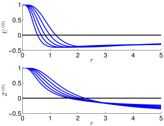
(a) Harmonic $k=0$

(b) Harmonic $k=1$

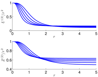
(c) Harmonic $k=2$

Figure 3. Index functions for the 3D supercritical NLS equation computed at six values of $.75\leq\sigma\leq 1.5$, inclusive.

4.1.2. Inner Products

Proposition 4.2.

Let $U_{1}^{(0)}$ and $U_{2}^{(0)}$, solve

(4.1a) $${\mathcal{L}}_{+}^{(0)}U_{1}^{(0)}=R$$

(4.1b) $${\mathcal{L}}_{+}^{(0)}U_{2}^{(0)}=\phi_{2}$$

And define:

(4.2a) $$K_{1}^{(0)} \equiv\left\langle{\mathcal{L}}_{+}^{(0)}U_{1}^{(0)},U_{1}^{(0)}\right\rangle,$$

(4.2b) $$K_{2}^{(0)} \equiv\left\langle{\mathcal{L}}_{+}^{(0)}U_{2}^{(0)},U_{2}^{(0)}\right\rangle,$$

(4.2c) $$K_{3}^{(0)} \equiv\left\langle{\mathcal{L}}_{+}^{(0)}U_{1}^{(0)},U_{2}^{(0)}\right\rangle.$$

The $K_{j}^{(0)}$ have the values indicated in Figure 4. Moreover, for $.8\leq\sigma\leq 1.2$,

(4.3) $$(K_{1}^{(0)}K_{2}^{(0)}-(K_{3}^{(0)})^{2})/K_{2}^{(0)}<0$$

as pictured in Figure 5.

Proof.

Proposition 3.6 ensures that the solutions exist. The boundary value problems and inner products were computed using the techniques described in Appendix A. The (4.2) and (4.3) were then computed at 41 uniformly spaced values of $\sigma$ between $.8$ and $1.2$. ∎

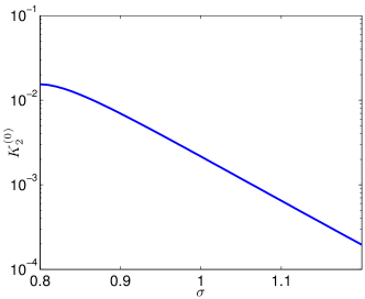
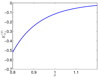
Figure 4. $K_{j}^{(0)}$ as functions of $\sigma$ for 3D supercritical NLS.

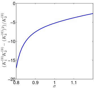
Figure 5. (4.3) as a function of $\sigma$ for 3D supercritical NLS.

Proposition 4.3.

Let $Z_{1}^{(0)}$ and $Z_{2}^{(0)}$, solve

(4.4a) $${\mathcal{L}}_{-}^{(0)}Z_{1}^{(0)}=\tfrac{1}{\sigma}R+rR^{\prime}$$

(4.4b) $${\mathcal{L}}_{-}^{(0)}Z_{2}^{(0)}=\phi_{1}$$

and define:

(4.5a) $$J_{1}^{(0)} \equiv\left\langle{\mathcal{L}}_{-}^{(0)}Z_{1}^{(0)},Z_{1}^{(0)}\right\rangle,$$

(4.5b) $$J_{2}^{(0)} \equiv\left\langle{\mathcal{L}}_{-}^{(0)}Z_{2}^{(0)},Z_{2}^{(0)}\right\rangle,$$

(4.5c) $$J_{3}^{(0)} \equiv\left\langle{\mathcal{L}}_{-}^{(0)}Z_{1}^{(0)},Z_{2}^{(0)}\right\rangle.$$

The $J_{j}^{(0)}$ have the values indicated in Figure 6. Moreover there exist $\sigma_{1}>.8$ and $\sigma_{2}>.8$ such that

(4.6) $$J_{1}^{(0)}<0,\quad\text{for $\sigma_{1}<\sigma<1.2$}$$

(4.7) $$(J_{1}^{(0)}J_{2}^{(0)}-(J_{3}^{(0)})^{2})/J_{2}^{(0)}<0,\quad\text{for $\sigma_{2}<\sigma<1.2$}$$

as pictured in Figure 7, where

(4.8a) $$\sigma_{1} =0.807699$$

(4.8b) $$\sigma_{2} =0.807425$$

Proof.

Like in the proof of Proposition 4.2, we numerically solve the boundary value problems at 41 uniformly spaced values of $\sigma$ between $.8$ and $1.2$. Using the root finding approach, discussed in Appendix A.3, we found the zero crossings, $\sigma_{1}$ and $\sigma_{2}$, of $J_{1}^{(0)}$ and (LABEL:e:nls3d_jprod2_0_var) to be at the indicated values. ∎

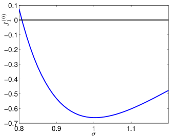
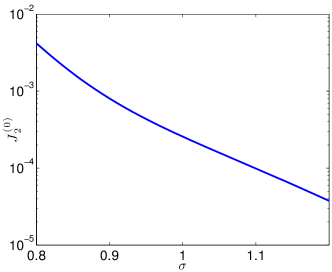
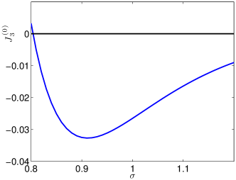
Figure 6. $J_{j}^{(0)}$ as functions of $\sigma$ for 3D supercritical NLS.

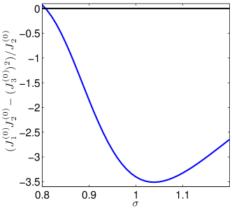
Figure 7. (4.7) as a function of $\sigma$ for 3D supercritical NLS.

Proposition 4.4.

Let $U_{1}^{(1)}$ solve

(4.9) $${\mathcal{L}}_{+}^{(1)}U_{1}^{(1)}=rR,\quad U_{1}^{(1)}\in L^{\infty}$$

Define

(4.10) $$K_{1}^{(1)}\equiv\left\langle{\mathcal{L}}_{+}^{(0)}U_{1}^{(1)},U_{1}^{(1)}\right\rangle$$

There exists $\sigma_{3}>.8$ such that

$$K_{1}^{(1)}<0,\quad\text{for $.8\leq\sigma<\sigma_{3}$}$$

as pictured in Figure 8, where

(4.11) $$\sigma_{3}=1.12092$$

Proof.

This is solved in the same manner as Propositions 4.2 and 4.3. ∎

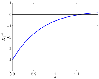
Figure 8. $K_{1}^{(1)}$ as a function of $\sigma$ for 3D supercritical NLS.

4.1.3. Proof of the Spectral Property

Subject to the acceptance of these computations, we are now in the position to prove the spectral property for

$$\sigma_{2}<\sigma<\sigma_{3}$$

where $\sigma_{2}$ and $\sigma_{3}$ are as defined by (4.8a) and (4.11). We first shall show that the bilinear form on each harmonic, $\bar{\mathcal{B}}_{\pm}^{(k)}$, is positive. We first prove the case of $\bar{\mathcal{B}}_{+}^{(0)}$.

Fixing $\sigma$, for a sufficiently small $\delta_{0}$, in the sense of Propositions 3.4 and 3.7,

$$\frac{1}{\bar{K}_{2}^{(0)}}\left(\bar{K}_{1}^{(0)}\bar{K}_{2}^{(0)}-(\bar{K}_{3}^{(0)})^{2}\right)<0.$$

where $\bar{K}_{j}^{(0)}$ is the inner product associated with the perturbed operator, $\bar{\mathcal{L}}_{+}^{(0)}$.

Given that $f$ is orthogonal to $R$ and $\phi_{2}$, it is orthogonal to any linear combination, including

$$\bar{q}=R-\frac{\bar{K}_{3}^{(0)}}{\bar{K}_{2}^{(0)}}\phi_{2}$$

Let $\bar{Q}$ solve

(4.12) $$\bar{\mathcal{L}}_{+}^{(0)}\bar{Q}=\bar{q}.$$

By construction,

(4.13) $$\bar{\mathcal{B}}_{+}^{(0)}(\bar{Q},\bar{Q})=\frac{1}{\bar{K}_{2}^{(0)}}\left(\bar{K}_{1}^{(0)}\bar{K}_{2}^{(0)}-(\bar{K}_{3}^{(0)})^{2}\right)<0.$$

To complete the proof of positivity, suppose $\bar{Q}\in H^{1}_{\mathrm{rad}}$, even thought it is not; it decays too slowly for $L^{2}$. We could decompose $H^{1}_{\mathrm{rad}}$ as

$$H^{1}_{\mathrm{rad}}={\mathrm{span}}\left\{\bar{Q}\right\}\oplus{\mathrm{span}}\left\{\bar{Q}\right\}^{\perp}$$

where the orthogonal decomposition is done with respect to $\bar{\mathcal{B}}_{+}^{(0)}$. We can do this because (4.13) implies the form is non-degenerate. Since ${\mathrm{ind}}({\mathcal{B}}_{+}^{(0)})=1$, ${\mathcal{B}}_{+}^{(0)}\geq 0$ on ${\mathrm{span}}\left\{\bar{Q}\right\}^{\perp}$. Were this not the case, it would yield a second negative direction, independent of $\bar{Q}$, contradicting the index computation.

Given $f\in H^{1}_{\mathrm{rad}}$, $f\perp R$ and $f\perp\phi_{2}$, with respect to $L^{2}$ orthogonality, $f$ is also $L^{2}$ orthogonal to $\bar{q}$. We might then decompose $f$ as proposed in the preceding paragraph

$$f=c\bar{Q}+f^{\perp},\quad\bar{{\mathcal{B}}}_{+}^{(0)}(f^{\perp},\bar{Q})=0.$$

If $c=0$, then $f=f^{\perp}$ resides in a subspace of $H^{1}_{\mathrm{rad}}$ where $\bar{{\mathcal{B}}}_{+}^{(0)}\geq 0$ , completing the proof. We now show $c=0$.

Taking the $L^{2}$ inner product of $f$ and $\bar{q}$,

$$\begin{split}0&=c\left\langle\bar{Q},q\right\rangle+\left\langle f^{\perp},\bar{q}\right\rangle=c\bar{\mathcal{B}}_{+}^{(0)}(\bar{Q},\bar{Q})+\left\langle u^{\perp},\bar{\mathcal{L}}_{+}^{(0)}\bar{Q}\right\rangle\\ &=c\bar{\mathcal{B}}_{+}^{(0)}(\bar{Q},\bar{Q})+{\mathcal{B}}_{+}^{(0)}(f^{\perp},\bar{Q})=c\bar{\mathcal{B}}_{+}^{(0)}(\bar{Q},\bar{Q})+0.\end{split}$$

Since we have computed ${\mathcal{B}}_{+}^{(0)}(\bar{Q},\bar{Q})\neq 0$, $c=0$. Hence, $L^{2}$ orthogonality to $\bar{q}$ induces $\bar{\mathcal{B}}_{+}^{(0)}$ orthogonality to $\bar{Q}$. Thus, $f$ lies in the positive subspace of $\bar{\mathcal{B}}_{+}^{(0)}$.

However, $\bar{Q}$ is not in $L^{2}$. To make this argument work, one can introduce a cutoff function and take an appropriate limit. We omit these details and refer the reader to [8, 12].

Positivity of $\bar{\mathcal{B}}_{-}^{(0)}$ is proven similarly. In this case, we use the $L^{2}$ orthogonality of $g$ to $\tfrac{1}{\sigma}R+rR^{\prime}$ and $\phi_{1}$. Indeed, we construct a new $\bar{Q}$, the solution to

$$\bar{\mathcal{L}}_{-}^{(0)}\bar{Q}=\tfrac{1}{\sigma}R+rR^{\prime}-\frac{\bar{J}_{3}^{(0)}}{\bar{J}_{2}^{(0)}}\phi_{1}$$

However, this is only successful for $\sigma_{2}<\sigma<1.2$.

Positivity of $\bar{\mathcal{B}}_{+}^{(1)}$ is somewhat easier, as there is no need to form a linear combination of elements; there is only one direction, $rR$, to project away from in this harmonic. $K_{1}^{(1)}<0$ for all the values of $.8\leq\sigma<\sigma_{3}$. We conclude that $L^{2}$ orthogonality of $f$ to $rR$ yields positivity. Since all other forms have index zero, there is nothing to prove for them.

We have now established that

(4.14) $$\bar{\mathcal{B}}({\bf z},{\bf z})\geq 0$$

since each form on each harmonic is positive. It is trivial to see that

(4.15) $${\mathcal{B}}({\bf z},{\bf z})\geq\delta_{0}\int e^{-\lvert\bf x\rvert}\lvert\bf z\rvert^{2}d{\bf x}.$$

This is almost the desired expression. Consider,

(4.16) $${\mathcal{B}}({\bf z},{\bf z})\geq\theta\left(\int\lvert\nabla{\bf z}\rvert^{2}-\lvert\mathcal{V}_{+}\rvert\lvert f\rvert^{2}-\lvert\mathcal{V}_{-}\rvert\lvert g\rvert^{2}d{\bf x}\right)+(1-\theta)\delta_{0}\int e^{-\lvert\bf x\rvert}\lvert{\bf z}\rvert^{2}d{\bf x}$$

for all $\theta\in(0,1)$. Both potentials satisfy the estimate $\lvert\mathcal{V}_{\pm}\rvert\lesssim e^{-2\sigma\lvert\bf x\rvert}$, $\sigma>\tfrac{1}{2}$, as $\lvert\bf x\rvert\to\infty$, so taking $\theta$ sufficiently small,

(4.17) $${\mathcal{B}}({\bf z},{\bf z})\geq\theta\int\lvert\nabla{\bf z}\rvert^{2}d{\bf x}+\frac{(1-\theta)\delta_{0}}{2}\int e^{-\lvert\bf x\rvert}\lvert{\bf z}\rvert^{2}d{\bf x}.$$

Hence,

$${\mathcal{B}}({\bf z},{\bf z})\gtrsim\int\left(\lvert\nabla{\bf z}\rvert^{2}+e^{-\lvert\bf x\rvert}\lvert{\bf z}\rvert^{2}\right)d{\bf x}$$

This proves the Spectral Property from which we then immediately get Theorem 1 for purely imaginary eigenvalues. As resonances in $d=3$ have sufficient decay, we can also rule them out.

4.2. 3D CQNLS

In this section we prove the Spectral Property for the 3D CQNLS equation. It is quite similar to 3D NLS, though we are now concerned with the values of $\gamma$ in (1.11) for which it holds.

4.2.1. Indexes

Proposition 4.5.

For $0\leq\gamma\leq.012$,

$${\mathrm{ind}}{\mathcal{L}}_{+}^{(0)}={\mathrm{ind}}{\mathcal{L}}_{-}^{(0)}={\mathrm{ind}}{\mathcal{L}}_{+}^{(1)}=1$$

$${\mathrm{ind}}{\mathcal{L}}_{+}^{(2)}={\mathrm{ind}}{\mathcal{L}}_{-}^{(1)}=0$$

Proof.

Examining Figures 9, we see that for three computed values of $0\leq\gamma\leq.012$, inclusive, we have the corresponding number of zero crossings. We argue by continuity that this should hold at all points in the interval. ∎

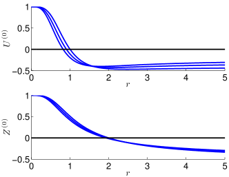
(a) Harmonic $k=0$

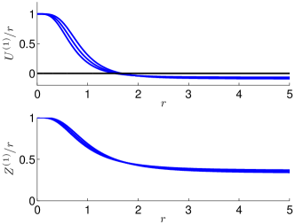
(b) Harmonic $k=1$

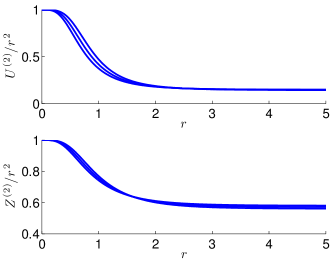
(c) Harmonic $k=2$

Figure 9. Index functions for the 3D CQNLS equation computed at three values of $0\leq\gamma\leq.012$, inclusive.

4.2.2. Inner Products

Proposition 4.6.

Let $U_{1}^{(0)}$ and $U_{2}^{(0)}$, solve

(4.18a) $${\mathcal{L}}_{+}^{(0)}U_{1}^{(0)}=R$$

(4.18b) $${\mathcal{L}}_{+}^{(0)}U_{2}^{(0)}=\phi_{2}$$

Define $K_{j}^{(0)}$ as in (4.2). The $K_{j}^{(0)}$ have the values indicated in Figure 10. Moreover, for $0\leq\gamma\leq 0.012$,

(4.19) $$(K_{1}^{(0)}K_{2}^{(0)}-(K_{3}^{(0)})^{2})/K_{1}^{(0)}<0$$

as pictured in Figure 11.

Proof.

As before, we prove this by direct computation, at twenty five values of $\gamma$ between $0$ and $.012$, inclusive. ∎

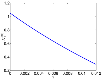
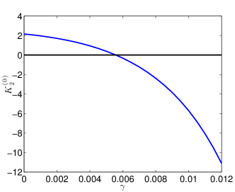
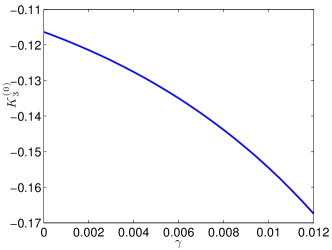
Figure 10. (4.2) as functions of $\gamma$ for 3D CQNLS.

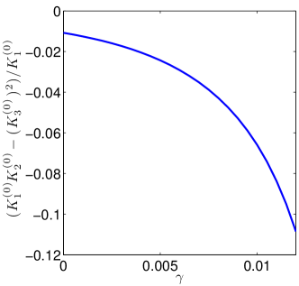
Figure 11. (4.19) as a function of $\gamma$ for 3D CQNLS.

Proposition 4.7.

Let $Z_{1}^{(0)}$ and $Z_{2}^{(0)}$, solve

(4.20a) $${\mathcal{L}}_{-}^{(0)}Z_{1}^{(0)}=\partial_{\omega}R$$

(4.20b) $${\mathcal{L}}_{-}^{(0)}Z_{2}^{(0)}=\phi_{1}$$

Define $J_{j}^{(0}$ as in (4.5). The $J_{j}^{(0)}$ have the values indicated in Figure 12. Moreover there exist $\gamma_{1}>0$ and $\sigma_{2}>0$ such that

(4.21) $$J_{1}^{(0)}<0,\quad\text{for $0\geq\gamma<\gamma_{1}$}$$

(4.22) $$(J_{1}^{(0)}J_{2}^{(0)}-(J_{3}^{(0)})^{2})/J_{2}^{(0)}<0,\quad\text{for $0\leq\gamma<\gamma_{2}$}$$

as pictured in Figure 13, where

(4.23a) $$\gamma_{1} =0.00989115$$

(4.23b) $$\gamma_{2} =0.0109065$$

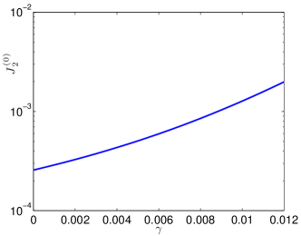
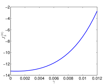
Figure 12. The $J_{j}^{(0)}$ as functions of $\gamma$ for 3D CQNLS.

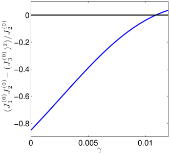
Figure 13. $(J_{1}^{(0)}J_{2}^{(0)}-(J_{3}^{(0)})^{2})/J_{2}^{(0)}$ as a function of $\gamma$ for 3D CQNLS.

Proposition 4.8.

Let $U_{1}^{(1)}$ solve

(4.24) $${\mathcal{L}}_{+}^{(1)}U_{1}^{(1)}=rR,\quad U_{1}^{(1)}\in L^{\infty}$$

Define $K_{1}^{(1)}$ as in (4.10). Then

$$K_{1}^{(1)}<0,\quad\text{for $0\leq\gamma 0.12$}$$

as pictured in Figure 14.

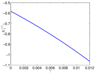
Figure 14. $K_{1}^{(1)}$ as a function of $\gamma$ for 3D CQNLS.

4.2.3. Proof of the Spectral Property

The proof is quite similar to that of 3D NLS and we omit many of the details. For a fixed $\gamma$ within the allowable range, we take $\delta_{0}$ sufficiently small so as not to alter the indexes or appreciably change the inner products.

A notable difference is that for $\bar{\mathcal{B}}_{+}^{(0)}$, we let $\bar{Q}$ solve

(4.25) $$\bar{\mathcal{L}}_{+}^{(0)}\bar{Q}=\bar{q}=-\frac{\bar{K}_{3}^{(0)}}{\bar{K}_{1}^{(0)}}R+\phi_{2}.$$

By construction and Proposition 4.6,

(4.26) $$\bar{\mathcal{B}}_{+}^{(0)}(\bar{Q},\bar{Q})=\frac{1}{K_{1}^{(0)}}\left(K_{1}^{(0)}K_{2}^{(0)}-\left(K_{3}^{(0)}\right)^{2}\right)<0.$$

If $f$ Is $L^{2}$ orthogonal to $R$ and $\phi_{2}$, then it is $L^{2}$ orthogonal to any linear combination. As before, this will induce ${\mathcal{B}}_{+}^{()}$ orthogonality to $\bar{Q}$, ensuring that ${\mathcal{B}}_{+}^{(0)}$ is positive for such $f$. This holds for all $0\leq\gamma<0.012$.

Positivity of $\bar{\mathcal{B}}_{-}^{(0)}$ is proven as before, except it only holds for $0\leq\gamma<\gamma_{2}$ due to the results of Proposition 4.7. Positivity of $\bar{\mathcal{B}}_{+}^{(1)}$ is the same, as are the rest of the forms, since they have index zero. This proves positivity of $\bar{\mathcal{B}}$ on $\mathcal{U}$, and the coercivity of ${\mathcal{B}}$ on $\mathcal{U}$ in the form of (1.17) follows as before. This yields Theorem 2.

4.3. 1D Supercritical NLS

In contrast to the 3D problems, where we decomposed into spherical harmonics, in 1D we decompose into even and odd functions.

4.3.1. Indexes

Proposition 4.9.

For $2.3\leq\sigma\leq 6.3$,

$${\mathrm{ind}}({\mathcal{B}}_{+}^{(e)})={\mathrm{ind}}({\mathcal{B}}_{-}^{(e)})={\mathrm{ind}}({\mathcal{B}}_{+}^{(o)})=1,\quad{\mathrm{ind}}({\mathcal{B}}_{-}^{(o)})=0$$

Proof.

As before, we prove this by direct computation. The index functions appear in Figure 15. ∎

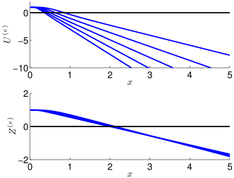
(a) Even Functions

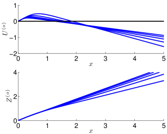
(b) Odd Functions

Figure 15. Index functions for the 1D supercritical NLS equation computed at five values of $2.3\leq\sigma\leq 6.3$, inclusive.

4.3.2. Inner Products

Proposition 4.10.

Let $U_{1}^{(0)}$ and $U_{2}^{(0)}$, solve

(4.27a) $${\mathcal{L}}_{+}^{(e)}U_{1}^{(e)}=R$$

(4.27b) $${\mathcal{L}}_{+}^{(e)}U_{2}^{(e)}=\phi_{2}$$

and define:

(4.28a) $$K_{1}^{(e)} \equiv\left\langle{\mathcal{L}}_{+}^{(e)}U_{1}^{(e)},U_{1}^{(e)}\right\rangle,$$

(4.28b) $$K_{2}^{(e)} \equiv\left\langle{\mathcal{L}}_{+}^{(e)}U_{2}^{(e)},U_{2}^{(e)}\right\rangle.$$

The $K_{j}^{(e)}$ have the values indicated in Figure 16. Moreover,

$$K_{1}^{(e)} <0,\quad\text{for $2.3\leq\sigma<\sigma_{4}$}$$

$$K_{2}^{(e)} <0,\quad\text{for $2.3\leq\sigma\leq 6.3$}$$

where

(4.29) $$\sigma_{4}=3.49928679909$$

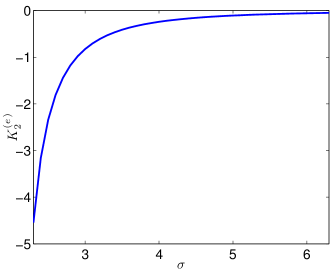
Figure 16. The $K_{j}^{(e)}$ as functions of $\sigma$ for 1D supercritical NLS.

Proposition 4.11.

Let $Z_{1}^{(e)}$ and $Z_{2}^{(e)}$, solve

(4.30a) $${\mathcal{L}}_{-}^{(e)}Z_{1}^{(e)} =\tfrac{1}{\sigma}R+xR^{\prime}$$

(4.30b) $${\mathcal{L}}_{-}^{(e)}Z_{2}^{(e)} =\phi_{1}$$

and define:

(4.31a) $$J_{1}^{(e)} \equiv\left\langle{\mathcal{L}}_{-}^{(e)}Z_{1}^{(e)},Z_{1}^{(e)}\right\rangle,$$

(4.31b) $$J_{2}^{(e)} \equiv\left\langle{\mathcal{L}}_{-}^{(e)}Z_{2}^{(e)},Z_{2}^{(e)}\right\rangle,$$

(4.31c) $$J_{3}^{(e)} \equiv\left\langle{\mathcal{L}}_{-}^{(e)}Z_{2}^{(e)},Z_{1}^{(e)}\right\rangle.$$

The $J_{j}^{(0)}$ have the values indicated in Figure 17. Moreover,

(4.32a) $$J_{1}^{(e)} <0,\quad\text{for $\sigma_{5}\leq\sigma\leq 6.3$},$$

(4.32b) $$(J_{1}^{(e)}J_{2}^{(e)}-(J_{3}^{(e)})^{2})/J_{2}^{(e)} <0,\quad\text{for $\sigma_{6}\leq\sigma\leq 6.3$},$$

where

(4.33a) $$\sigma_{5} =2.45649878,$$

(4.33b) $$\sigma_{6} =2.45379561.$$

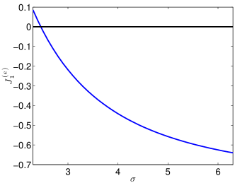
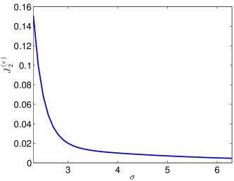
Figure 17. (4.31) as functions of $\sigma$ for 1D supercritical NLS.

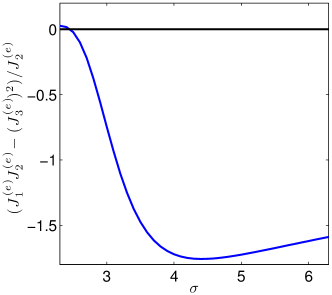
Figure 18. (4.32b) as a function of $\sigma$ for 1D supercritical NLS.

Proposition 4.12.

Let $U_{1}^{(o)}$ solve

(4.34) $${\mathcal{L}}_{+}^{(o)}U_{1}^{(o)}=xR$$

and define

(4.35) $$K_{1}^{(o)}\equiv\left\langle{\mathcal{L}}_{+}^{(o)}U_{1}^{(o)},U_{1}^{(o)}\right\rangle.$$

$K_{1}^{(o)}$ has the values indicated in Figure 19. Moreover,

$$K_{1}^{(o)}<0,\quad\text{for $2.3\leq\sigma\leq\sigma_{7}$}\\$$

where

(4.36) $$\sigma_{7}=6.1288520139$$

Figure 19. $K_{1}^{(1)}$ as a function of $\sigma$ for 1D supercritical NLS.

4.3.3. Proof of the Spectral Property

To prove the spectral property in this case, we can use the orthogonality of $f$ to $\phi_{2}$ to induce positivity of ${\mathcal{B}}_{+}^{(e)}$ for all $2.3\leq\sigma\leq 6.3$, via Proposition 4.10. For ${\mathcal{B}}_{-}^{(e)}$, $L^{2}$ orthogonality to $\tfrac{1}{\sigma}R+xR^{\prime}$ and $\phi_{1}$ induces positivity for $\sigma_{6}<\sigma\leq 6.3$ through Proposition 4.11. Finally, Proposition 4.12 yields positivity of ${\mathcal{B}}_{+}^{(o)}$ for $2.3\leq\sigma<\sigma_{7}$.

5. Discussion

We have successfully proven there are no purely imaginary eigenvalues, both in the spectral gap and embedded in the essential spectrum, for a collection of a orbitally unstable solitary wave solutions of NLS. However, there is still much to be done. First, the range of orbitally unstable solitary waves has not been exhausted. We know there are no purely imaginary eigenvalues for $\sigma>2$ in the 1D NLS equation, and we anticipate that there are none for $\sigma>2/3$ in 3D. We expect similar results for the entire unstable branch of CQNLS. Second, we have shown that the threshold found in [6], given by (1.10), is suboptimal; our range, (1.12), is larger, but it too is likely suboptimal.

This work also raises questions of what is satisfactory for a rigorous proof. We relied on the computer in the following steps:

• Computing the solitary waves for the 3D, a nonlinear boundary value problem on an unbounded domain;

• Computing a finite number of index functions, linear initial value problems on unbounded domains;

• Solving a finite collection of linear elliptic problems on unbounded domains;

• Computing inner products on an unbounded intervals.

To deal with these obstacles we truncated the intervals to $[0,r_{\max}]$ ($[0,x_{\max}]$ in 1D), and introduced a finite number of discretization points within the intervals. Even with these computations, we have only established the results for isolated values of $\sigma$ or $\gamma$; we argue by continuity that the results should extend to continuous intervals.

However, we are able to produce a variety of consistency and a posteriori checks, such as verifying that the artificial boundary conditions are being satisfied sufficiently well. Despite our confidence in our computations, it would still be desirable to avoid the use of the computer. Indeed, an alternative method may permit us to move beyond the seemingly artificial restrictions on $\sigma$ and $\gamma$ of our results.

Appendix A Numerical Methods

The codes used to produce the results appearing in this work are available at http://www.math.toronto.edu/simpson/files/spec_prop_asad_simpson_code.zip for examination, verification, and experimentation.

The numerical methods we use are the same as those used in [12], and separately in Simpson & Zwiers, [20]. For the 3D problems, we use the Fortran 90/95 based boundary value problem solver of Shampine, Muir, & Xu, [19]. For the 1D problems, we found it sufficient to use the closely related bvp4c routine in Matlab , [17, 18]. These algorithms require us to specify the problems as first order systems of the form

$$\frac{d}{dr}{\bf y}=\tfrac{1}{r}S{\bf y}+{\bf f}(r,{\bf y})$$

where $S$ is a constant matrix and ${\bf f}$ contains all non-singular terms, both linear and nonlinear.

This automatically accommodates problems involving $r^{-1}$ type singularities at the origin, as found in the equation for the 3D solitons and the $k=0$ harmonic boundary value problems. For higher harmonics, we use a point transformation $W(r)=r^{k}\tilde{W}(r)$ to transform

$$\left[-\frac{d^{2}}{dr^{2}}-\frac{d-1}{r}\frac{d}{dr}+\frac{k(k+d-2)}{r^{2}}\right]W\Rightarrow r^{k}\left[-\frac{d^{2}}{dr^{2}}-\frac{d-1+2k}{r}\frac{d}{dr}\right]\tilde{W}.$$

A.1. Index Functions

For the 3D problems, we computed the index functions on the domain $[0,200]$ with a tolerance setting of $10^{-13}$. The 1D problems were computed on the domain $[0,100]$ with absolute and relative tolerances of $10^{-13}$. While Figures 3, 9, and 15 show the indicated numbers of roots, they obviously do not prove that there is no root at some larger value of $x$ or $r$.

To mitigate this uncertainly, there are two things we can check. First, we can examine the solution on a much larger domain. A more systematic approach is to note that since the potentials are highly localized, asymptotically, the index functions satisfy the estimates

(A.1a) $$U^{(k)}(r) \approx C_{0}^{(k)}r^{k}+C_{1}^{(k)}r^{2-d-k}$$

(A.1b) $$Z^{(k)}(r) \approx D_{0}^{(k)}r^{k}+D_{1}^{(k)}r^{2-d-k}$$

where $C_{j}^{(k)}$ and $D_{j}^{(k)}$ are constants. Estimating these constants, and seeing that they have the correct signs and magnitudes, indicates that there cannot be further roots. For example, in Figure 20, we see that $C_{0}^{(0)}\approx-0.3668$ and $C_{1}^{(0)}\approx-0.2393$. The only root of

$$-0.3668-0.2393/r$$

is near $-0.65$. Thus, there should be no zeros in the “far field”. Similar analysis works for the $D_{j}^{(0)}$ constants.

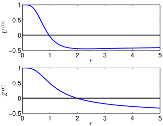
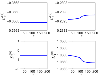
Figure 20. The index functions and the asymptotic constants for the $\gamma=.01$ case of CQNLS in harmonic $k=0$.

A.2. Boundary Value Problems & Artificial Boundary Conditions

Since this algorithm requires us to compute on a finite domain, $[0,{r_{\max}}]$, we must introduce artificial boundary conditions at $r_{\max}$. These are discussed in the above references, but include

$$R(r_{\max})+\frac{r_{\max}}{1+r_{\max}}R^{\prime}(r_{\max})=0$$

$$\partial_{\omega}|_{\omega=1}R(r_{\max})+\partial_{\omega}|_{\omega=1}R^{\prime}(r_{\max})=0$$

for the 3D problems. Again, additional details are given in [12, 20]. An example of an a posteriori check of these being satisfied is given in Figure 21, which includes computations of the soliton, the unstable eigenstate, and the solutions of the boundary value problems for Proposition 4.6.

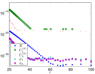
Figure 21. Verification of the artificial boundary conditions for the soliton, $R$, the eigenstate, $\boldsymbol{\phi}$, and the solutions of the boundary value problems $U^{(0)}_{j}$ for the $\gamma=0.01$ case of CQNLS.

The boundary value problems were solved on the domain $[0,100]$ in all cases. For the 3D problems, the tolerance was set at $10^{-12}$. for the 1D problems, the absolute tolerance was $10^{-8}$ and relative tolerance was $10^{-10}$.

A.3. Root Finding

To compute roots of the inner products, or combinations of them, we wrap our routines within the fzero routine, with default settings, of Matlab ; we define a function that, for a given value of $\sigma$ or $\gamma$, returns the inner product, and pass this to fzero. We found this could provide approximately six digits of accuracy in our 3D computations, notably for the bounds (1.12) and (1.13), while for the 1D computations, we were able to get eleven digits.

There appears to be a loss of sensitivity to the input $\sigma$ or $\gamma$ for the 3D problems. An example of this appears in Figure 22, where we see that for a range of $\sigma$ values near the root, $J_{1}^{(0)}$ is piecewise constant. Refinements to our approach, with higher order corrections to the artificial boundary conditions, may improve the accuracy.

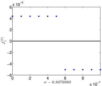
Figure 22. Zooming in on the root of $J_{1}^{(0)}$ inner product of the 3D NLS equation, the solution is appears piecewise constant. This is a closeup of Figure 6(a).

References

- [1] V. S. Buslaev and G. S. Perel′man. On the stability of solitary waves for nonlinear Schrödinger equations. In Nonlinear evolution equations, volume 164 of Amer. Math. Soc. Transl. Ser. 2, pages 75–98. Amer. Math. Soc., Providence, RI, 1995.
- [2] V. S. Buslaev and C. Sulem. On asymptotic stability of solitary waves for nonlinear schrödinger equations. Ann. Inst. H. Poincaré Anal. Non Linéaire, 20(3):419–475, 2003.
- [3] S. Cuccagna. On asymptotic stability of ground states of NLS. Rev. Math. Phys., 15(8):877–903, 2003.
- [4] S. Cuccagna and D. Pelinovsky. Bifurcations from the endpoints of the essential spectrum in the linearized nonlinear Schrödinger problem. J. Math. Phys., 46(5):053520, 15, 2005.
- [5] S. Cuccagna, D. Pelinovsky, and V. Vougalter. Spectra of positive and negative energies in the linearized NLS problem. Comm. Pure Appl. Math., 58(1):1–29, 2005.
- [6] L. Demanet and W. Schlag. Numerical verification of a gap condition for a linearized nonlinear Schrödinger equation. Nonlinearity, pages 829–852, 2006.
- [7] M. B. Erdogan and W. Schlag. Dispersive estimates for schrödinger operators in the presence of a resonance and/or an eigenvalue at zero energy in dimension three. ii. Journal d’Analyse Mathématique, 99:199–248, 2006.
- [8] G. Fibich, F. Merle, and P. Raphaël. Proof of a Spectral Property related to the singular formation for the critical nonlinear Schrödinger equation. Physica D, 220:1–13, 2006.
- [9] M. Grillakis, J. Shatah, and W. Strauss. Stability theory of solitary waves in the presence of symmetry. i. J Funct Anal, 74(1):160–197, 1987.
- [10] M. Grillakis, J. Shatah, and W. Strauss. Stability theory of solitary waves in the presence of symmetry. ii. J Funct Anal, 94(2):308–348, 1990.
- [11] J. Krieger and W. Schlag. Stable manifolds for all monic supercritical focusing nonlinear Schrödinger equations in one dimension. J. Amer. Math. Soc., 19(4):815–920, 2006.
- [12] J. L. Marzuola and G. Simpson. Spectral analysis for matrix hamiltonian operators. Nonlinearity, 24:389–429, 2011.
- [13] F. Merle and P. Raphael. The blow-up dynamic and upper bound on the blow-up rate for critical nonlinear Schrödinger equation. Annals of Mathematics, pages 157–222, 2005.
- [14] G. Perelman. Personal communication to Wilhelm Schlag.
- [15] I. Rodnianski, W. Schlag, and A. Soffer. Asymptotic stability of -soliton states of NLS. Preprint, 2003.
- [16] W. Schlag. Stable manifolds for an orbitally unstable nonlinear schrödinger equation. Ann. of Math. (2), 169(1):139–227, 2009.
- [17] L. Shampine. Singular boundary value problems for ODEs. Applied Mathematics and Computation, 138(1):99–112, 2003.
- [18] L. Shampine, I. Gladwell, and S. Thompson. Solving ODEs with MATLAB. Cambridge University Press, 2003.
- [19] L. Shampine, P. Muir, and H. Xu. A User-Friendly Fortran BVP Solver. JNAIAM, 1(2):201–217, 2006.
- [20] G. Simpson and I. Zwiers. Vortex collapse for the l2-critical nonlinear schrödinger equation. arXiv, math.AP, Oct 2010. 36 pages, 10 figures.
- [21] C. Sulem and P. Sulem. The Nonlinear Schrödinger Equation: Self-Focusing and Wave Collapse. Springer, 1999.
- [22] M. I. Weinstein. Modulational stability of ground states of nonlinear schrödinger equations. SIAM Journal on Mathematical Analysis, 16:472, 1985.
- [23] M. I. Weinstein. Lyapunov stability of ground states of nonlinear dispersive evolution equations. Communications on Pure and Applied Mathematics, pages 51–68, 1986.