22institutetext: Agenzia Spaziale Italiana Science Data Center, c/o ESRIN, via Galileo Galilei, Frascati, Italy
33institutetext: Agenzia Spaziale Italiana, Viale Liegi 26, Roma, Italy
44institutetext: Astroparticule et Cosmologie, CNRS (UMR7164), Université Denis Diderot Paris 7, Bâtiment Condorcet, 10 rue A. Domon et Léonie Duquet, Paris, France
55institutetext: Australia Telescope National Facility, CSIRO, P.O. Box 76, Epping, NSW 1710, Australia
66institutetext: CNR - ISTI, Area della Ricerca, via G. Moruzzi 1, Pisa, Italy
77institutetext: CNRS, IRAP, 9 Av. colonel Roche, BP 44346, F-31028 Toulouse cedex 4, France
88institutetext: California Institute of Technology, Pasadena, California, U.S.A.
99institutetext: Centre of Mathematics for Applications, University of Oslo, Blindern, Oslo, Norway
1010institutetext: DTU Space, National Space Institute, Juliane Mariesvej 30, Copenhagen, Denmark
1111institutetext: Departamento de Física, Universidad de Oviedo, Avda. Calvo Sotelo s/n, Oviedo, Spain
1212institutetext: Departamento de Matemáticas, Estadística y Computación, Universidad de Cantabria, Avda. de los Castros s/n, Santander, Spain
1313institutetext: Department of Physics & Astronomy, University of British Columbia, 6224 Agricultural Road, Vancouver, British Columbia, Canada
1414institutetext: Department of Physics and Astronomy, University of Southern California, Los Angeles, California, U.S.A.
1515institutetext: Department of Physics, Gustaf Hällströmin katu 2a, University of Helsinki, Helsinki, Finland
1616institutetext: Department of Physics, University of California, Berkeley, California, U.S.A.
1717institutetext: Department of Physics, University of California, One Shields Avenue, Davis, California, U.S.A.
1818institutetext: Department of Physics, University of California, Santa Barbara, California, U.S.A.
1919institutetext: Department of Physics, University of Oxford, 1 Keble Road, Oxford, U.K.
2020institutetext: Dipartimento di Fisica G. Galilei, Università degli Studi di Padova, via Marzolo 8, 35131 Padova, Italy
2121institutetext: Dipartimento di Fisica, Università La Sapienza, P. le A. Moro 2, Roma, Italy
2222institutetext: Dipartimento di Fisica, Università degli Studi di Milano, Via Celoria, 16, Milano, Italy
2323institutetext: Dipartimento di Fisica, Università degli Studi di Trieste, via A. Valerio 2, Trieste, Italy
2424institutetext: Dipartimento di Fisica, Università di Ferrara, Via Saragat 1, 44122 Ferrara, Italy
2525institutetext: Dipartimento di Fisica, Università di Roma Tor Vergata, Via della Ricerca Scientifica, 1, Roma, Italy
2626institutetext: Dipartimento di Matematica, Università di Roma Tor Vergata, Via della Ricerca Scientifica, 1, Roma, Italy
2727institutetext: Dpto. Astrofísica, Universidad de La Laguna (ULL), E-38206 La Laguna, Tenerife, Spain
2828institutetext: European Space Agency, ESAC, Planck Science Office, Camino bajo del Castillo, s/n, Urbanización Villafranca del Castillo, Villanueva de la Cañada, Madrid, Spain
2929institutetext: European Space Agency, ESTEC, Keplerlaan 1, 2201 AZ Noordwijk, The Netherlands
3030institutetext: Haverford College Astronomy Department, 370 Lancaster Avenue, Haverford, Pennsylvania, U.S.A.
3131institutetext: Helsinki Institute of Physics, Gustaf Hällströmin katu 2, University of Helsinki, Helsinki, Finland
3232institutetext: INAF - Osservatorio Astrofisico di Arcetri, Largo Enrico Fermi 5, Firenze, Italy
3333institutetext: INAF - Osservatorio Astrofisico di Catania, Via S. Sofia 78, Catania, Italy
3434institutetext: INAF - Osservatorio Astronomico di Padova, Vicolo dell’Osservatorio 5, Padova, Italy
3535institutetext: INAF - Osservatorio Astronomico di Roma, via di Frascati 33, Monte Porzio Catone, Italy
3636institutetext: INAF - Osservatorio Astronomico di Trieste, Via G.B. Tiepolo 11, Trieste, Italy
3737institutetext: INAF/IASF Bologna, Via Gobetti 101, Bologna, Italy
3838institutetext: INAF/IASF Milano, Via E. Bassini 15, Milano, Italy
3939institutetext: INRIA, Laboratoire de Recherche en Informatique, Université Paris-Sud 11, Bâtiment 490, 91405 Orsay Cedex, France
4040institutetext: ISDC Data Centre for Astrophysics, University of Geneva, ch. d’Ecogia 16, Versoix, Switzerland
4141institutetext: Infrared Processing and Analysis Center, California Institute of Technology, Pasadena, CA 91125, U.S.A.
4242institutetext: Institut d’Astrophysique Spatiale, CNRS (UMR8617) Université Paris-Sud 11, Bâtiment 121, Orsay, France
4343institutetext: Institut d’Astrophysique de Paris, CNRS UMR7095, Université Pierre & Marie Curie, 98 bis boulevard Arago, Paris, France
4444institutetext: Institute of Astronomy, University of Cambridge, Madingley Road, Cambridge CB3 0HA, U.K.
4545institutetext: Institute of Theoretical Astrophysics, University of Oslo, Blindern, Oslo, Norway
4646institutetext: Instituto de Astrofísica de Canarias, C/Vía Láctea s/n, La Laguna, Tenerife, Spain
4747institutetext: Instituto de Física de Cantabria (CSIC-Universidad de Cantabria), Avda. de los Castros s/n, Santander, Spain
4848institutetext: Jet Propulsion Laboratory, California Institute of Technology, 4800 Oak Grove Drive, Pasadena, California, U.S.A.
4949institutetext: Jodrell Bank Centre for Astrophysics, Alan Turing Building, School of Physics and Astronomy, The University of Manchester, Oxford Road, Manchester, M13 9PL, U.K.
5050institutetext: LERMA, CNRS, Observatoire de Paris, 61 Avenue de l’Observatoire, Paris, France
5151institutetext: Lawrence Berkeley National Laboratory, Berkeley, California, U.S.A.
5252institutetext: Max-Planck-Institut für Astrophysik, Karl-Schwarzschild-Str. 1, 85741 Garching, Germany
5353institutetext: MilliLab, VTT Technical Research Centre of Finland, Tietotie 3, Espoo, Finland
5454institutetext: SISSA, Astrophysics Sector, via Bonomea 265, 34136, Trieste, Italy
5555institutetext: Space Sciences Laboratory, University of California, Berkeley, California, U.S.A.
5656institutetext: Spitzer Science Center, 1200 E. California Blvd., Pasadena, California, U.S.A.
5757institutetext: Université de Toulouse, UPS-OMP, IRAP, F-31028 Toulouse cedex 4, France
5858institutetext: Warsaw University Observatory, Aleje Ujazdowskie 4, 00-478 Warszawa, Poland
Planck early results. V. The Low Frequency Instrument data processing
We describe the processing of data from the Low Frequency Instrument (LFI) used in production of the Planck Early Release Compact Source Catalogue (ERCSC). In particular, we discuss the steps involved in reducing the data from telemetry packets to cleaned, calibrated, time-ordered data (TOD) and frequency maps. Data are continuously calibrated using the modulation of the temperature of the cosmic microwave background radiation induced by the motion of the spacecraft. Noise properties are estimated from TOD from which the sky signal has been removed using a generalized least square map-making algorithm. Measured noise knee-frequencies range from mHz at 30 GHz to a few tens of mHz at 70 GHz. A destriping code (Madam) is employed to combine radiometric data and pointing information into sky maps, minimizing the variance of correlated noise. Noise covariance matrices required to compute statistical uncertainties on LFI and Planck products are also produced. Main beams are estimated down to the dB level using Jupiter transits, which are also used for geometrical calibration of the focal plane.
Key Words.:
methods: data analysis - cosmic background radiation - cosmology: observations - surveys1 Introduction
Planck111Planck (http://www.esa.int/Planck) is a project of the European Space Agency (ESA) with instruments provided by two scientific consortia funded by ESA member states (in particular the lead countries France and Italy), with contributions from NASA (USA) and telescope reflectors provided by a collaboration between ESA and a scientific consortium led and funded by Denmark. (Tauber et al. 2010; Planck Collaboration 2011a) is a third generation space mission to measure the anisotropy of the Cosmic Microwave Background (CMB). It observes the sky in nine frequency bands covering 30–857 GHz with high sensitivity and angular resolution from 31′to 5′. The Low Frequency Instrument (LFI) (Mandolesi et al. 2010; Bersanelli et al. 2010; Mennella et al. 2011) covers the 30, 44, and 70 GHz bands with amplifiers cooled to 20 K. The High Frequency Instrument (HFI) (Lamarre et al. 2010; Planck HFI Core Team 2011a) covers the 100, 143, 217, 353, 545, and 857 GHz bands with bolometers cooled to 0.1 K. Polarization is measured in all but the highest two bands (Leahy et al. 2010; Rosset et al. 2010). A combination of radiative cooling and three mechanical coolers produces the temperatures needed for the detectors and optics (Planck Collaboration 2011b). Two Data Processing Centres (DPCs), conceived as interacting and complementary since the earliest design of the Planck scientific ground segment (Pasian & Gispert 2000); check and calibrate the data and make maps of the sky, this paper and (Planck HFI Core Team 2011b). Planck’s sensitivity, angular resolution, and frequency coverage make it a powerful instrument for galactic and extragalactic astrophysics, as well as cosmology. Early astrophysics results are given in Planck Collaboration, 2011c–z.
The Low Frequency Instrument LFI on Planck comprises a set of 11 radiometer chain assemblies (RCAs), each composed of two independent, pseudo-correlation radiometers. There are two RCAs at 30 GHz, three at 44 GHz, and six at 70 GHz. Each radiometer has two independent diodes for detection, integration, and conversion from radio frequency signal to DC voltage. The LFI is cryogenically cooled to 20 K to reduce noise, while the pseudo-correlation design with reference loads at 4 K ensures good suppression of noise (Mennella et al. 2011).
LFI produces full-sky maps centered near 30, 44, and 70 GHz, with significant improvements with respect to current CMB data in the same frequency range. Careful data processing is required in order to realize the full potential of LFI and the ambitious science goals of Planck, which require that systematic effects be limited to a few K per resolution element.
In this paper we describe the processing steps implemented to create LFI data products, with particular attention to the needs of the first set of astrophysics results.
The structure of the paper follows the flow of the data through the analysis pipeline. Section 2 describes the creation of time ordered information (TOI) from telemetry packets, time stamping, pointing reconstruction, and data flagging. Section 3 describes the main operations performed on the TOI, including removal of frequency spikes, creation of differenced data, determination of the gain modulation factor, and diode combination. Beam reconstruction is discussed in Sect. 4, calibration in Sect. 5, and noise in Sect. 6. Map-making, covariance matrices, and tests based on jackknife analysis and Monte Carlo simulations are described in Sect. 7. Section 8 reports on colour corrections. Section 9 describes how the CMB was removed from LFI and HFI maps. Finally, Sect. 10 gives an overview of the software infrastructure at the LFI DPC.
2 Creation of time ordered information
The task of the Level 1 DPC pipeline is to retrieve all necessary information from packets received each day from the Mission Operations Centre (MOC) and to transform the scientific TOI and housekeeping (H/K) data into a form that is manageable by the scientific pipeline.
During the 3 h daily telecommunication period (DTCP), the MOC receives telemetry from the previous day, archived in on-board mass memory, together with real-time telemetry. Additional auxiliary files, such as the attitude history file (AHF) of the satellite, are produced.
The MOC consolidates the data for each day, checking for gaps or corrupted telemetry packets, then provides the data, together with additional auxiliary data, to the DPCs through a client/server application called the data disposition system (DDS).
The data are received at the DPC as a stream of packets, which are handled automatically by four Level 1 pipelines: Data Receipt, Telemetry Handling, Auxiliary Data, and Command History.
The Data Receipt pipeline implements the client side of the interface with the DDS. It requests a subset of data provided through this interface. A finite-state machine model has been used in the design of this pipeline for better formalization of the actions required during interaction with the DDS server.
The Telemetry Handling pipeline is triggered when a new segment of telemetry data is received. The first task (Telemetry Unscrambler) discriminates between scientific and housekeeping telemetry packets. Scientific packets are grouped according to radiometer, detector source, and processing type, then uncompressed and decoded (see next paragraph). The on-board time of each sample is computed based on the packet on-board time and the detector sampling frequency. Housekeeping telemetry packets are also grouped according to packet type, and each housekeeping parameter within the packet is extracted and saved into TOI. Subsequent tasks of the pipeline perform calibration of housekeeping and scientific TOIs together with additional quality checks (e.g., out of limits, time correlation). The last task, FITS2DMC, ingests the TOIs into the Data Management Component (DMC), making them available to the Level 2 and Level 3 pipelines.
The Auxiliary Data pipeline ingests the AHF provided by Flight Dynamics into the DMC. Finally the Command History pipeline requests and stores the list of telecommands sent to the satellite during the DTCP.
The four pipelines are implemented as perl scripts, scheduled every 5 min. Trigger files are created to activate the processing in the Auxiliary Data and Command History pipelines, and a pipeline monitoring facility displays information about the status of each pipeline. The entire Level 1 pipeline was heavily tested and validated before the start of Planck operations (see Frailis et al. 2009, for more details).
2.1 Scientific data processing
When creating TOI, the Level 1 pipeline must recover accurately the values of the original (averaged) sky and load samples acquired on-board. The instrument can acquire scientific data in several modes or “PTypes”; we describe here only the nominal one (PType 5) (see Zacchei et al. 2009). The key feature is that two independent differenced time streams are created from the sky and load signals with two different gain modulation factors (GMFs).
Data of PType 5 are first uncompressed. The lossless compression applied on-board is inverted, and the number of samples obtained is checked against auxiliary packet information. Decompressed data are then subject to a dequantization step to recover the original signals according to
| (1) |
where and are parameters of the readout electronics box assembly (REBA), calibration of which is described by Maris et al. (2009).
After dequantization, data are demixed to obtain and using as inputs the gain modulation factors and determined during REBA calibration (Maris et al. 2009):
| (2) |
| (3) |
Conversion from ADU (analog-to-digital units) to volts is achieved by
| (4) |
where , , and are data acquisition electronics (DAE) gain, offset, and small tunable offset, respectively, whose optimal values were determined during ground tests (Maris et al. 2009).
2.2 On-Board Time reconstruction
A time stamp is assigned to each data sample. If the phase switch (Mennella et al. 2011) is off (not switching), the packet contains consecutive values of either sky or load samples. Then
| (5) |
where is the sample index within the packet and is the mean time stamp of the first averaged sample. is the number of fast samples averaged together to obtain a single detector sample, and kHz is the detector sampling frequency.
If the phase switch is on (nominal case), consecutive pairs of either skyload or loadsky samples are stored in the packet. Then consecutive pairs of samples have the same time stamp and
| (6) |
On-board time information is stored in the form of TOI and directly linked to its scientific sample.
2.3 Data flagging
For each sample we define a 32-bit flag mask to identify potential inconsistencies in the data and to enable the pipeline to skip that sample or handle it differently during further processing. Currently flags that are checked include: those identifying the stable pointing period (determined from the AHF); science data that cannot be recovered (e.g., because of saturation); samples artificially created to fill data gaps; and samples affected by planet transits and moving objects within the Solar system.
3 TOI processing
3.1 Electronic spikes
The clock in the housekeeping electronics is inadequately shielded from the data lines, resulting in noise “spikes” in the frequency domain at multiples of 1 Hz (Meinhold et al. 2009). The spikes are synchronous with the on-board time, with no change in phase over the entire survey, allowing construction of a piecewise-continuous template by summing the data for a given detector onto a one second interval (Fig. 1) The amplitude and shape differ from detector to detector; differences between detectors of different frequency tend to be larger than between those of the same frequency. The amplitude also varies with time. This variation is estimated by constructing templates like Fig. 1 summed over the entire survey to obtain the shape of the signal, and then fitting the amplitude of a signal of this shape for each hour of data. This amplitude is smoothed with a 20-day boxcar window function to reduce the noise. Because of noise, this is likely to be an overestimate of the true variations.
To estimate the effect of spikes on the science data, we generate three simulated maps at each frequency. The first is a noise map, generated from the instrument white noise levels as measured in the data and the scan strategy of Planck, but no spikes or correlated noise. This is a best case scenario, with the lowest noise level possible in a real map. The second is a “spike” map, calculated assuming the square wave template for each detector modulated by a time-varying amplitude measured from the data, as described above. Because the variation of amplitudes is an overestimate, as described above, this is a worst-case scenario of the effect of spikes. The third map is a “spike-subtracted” map, the same as the second, but with a constant spike template subtracted. This gives an estimate of the residual effect of electronic spikes that would be left in the maps if the spike template were subtracted. The 30 GHz maps are at HEALPix resolution ; the 44 GHz and 70 GHz maps were produced at .
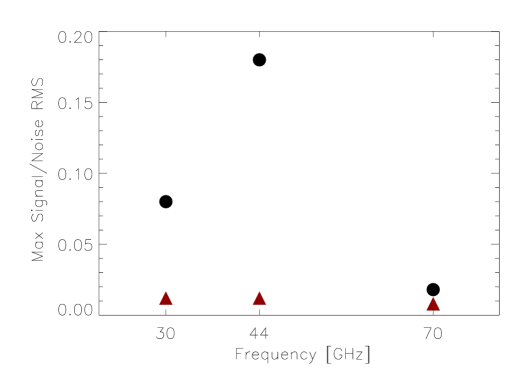
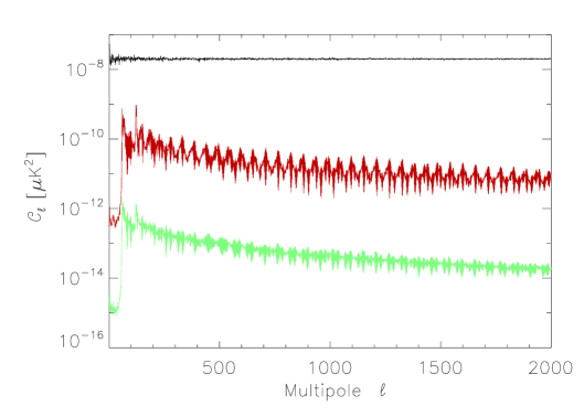
We scale the spike and spike subtracted maps to the noise, i.e., Map2/rms(Map3) and Map2/rms(Map3), where the rms is calculated from the global rms of the noise map scaled as appropriate for the relative number of observations (“hits”) in that pixel. Figure 2 (left) shows the maximum value of these ratios over the whole sky. At 44 GHz, the most affected frequency, the effect in the worst pixel is less than 20% of the noise. At 70 GHz the effect in the worst pixel is an insignificant 2% of the noise.
Figure 2 (right) gives angular power spectra of the three 44 GHz maps. The effect is everywhere well below the noise, and subtraction of a constant amplitude square-wave template reduces the effect by almost two orders of magnitude.
We decided to remove a square-wave template only at 44 GHz. This reduces the spike residual from 20% of the noise to 1% of the noise. At 70 GHz the effect of spikes is extremely small without correction, and at 30 GHz uncertainty in the template combined with the small size of the effect argued against removal.
3.2 Gain modulation factor and differenced data
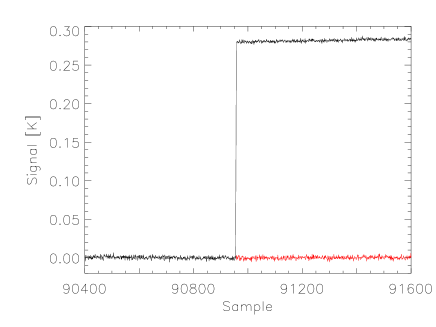
The output of each detector (diode) switches at 4096 Hz (Mennella et al. 2010) between the sky, , and the 4 K reference load, . and are dominated by noise, with knee frequencies of tens of hertz. This noise is highly correlated between the two streams, a result of the pseudo-correlation design (Bersanelli et al. 2010), and differencing the streams results in a dramatic reduction of the noise. The two arms of the radiometer are slightly unbalanced, as one looks at the 2.7 K sky and the other looks at the K reference load. To force the mean of the difference to zero, the load signal is multiplied by the GMF, , which can be computed in several ways (Mennella et al. 2003). The simplest method, and the one implemented in the processing pipeline, is to take the ratio of DC levels from sky and load outputs obtained by averaging the two time streams, i.e., . Then
| (7) |
We compute from unflagged data for each pointing period identified from the AHF information.
To verify the accuracy of this approach, we started with a time stream of real differenced data, then generated two time streams of undifferenced data using a constant (typical) value of . We then ran these two time streams through the pipeline, and compared the results with the original time stream. Deviations between the pipeline values of and the constant input value used to generate the undifferenced data were at the 0.002% level.
The factor has been stable over the mission so far, with overall variations of 0.03–0.04%. To keep the pipeline simple, we apply a single value of to each pointing period.
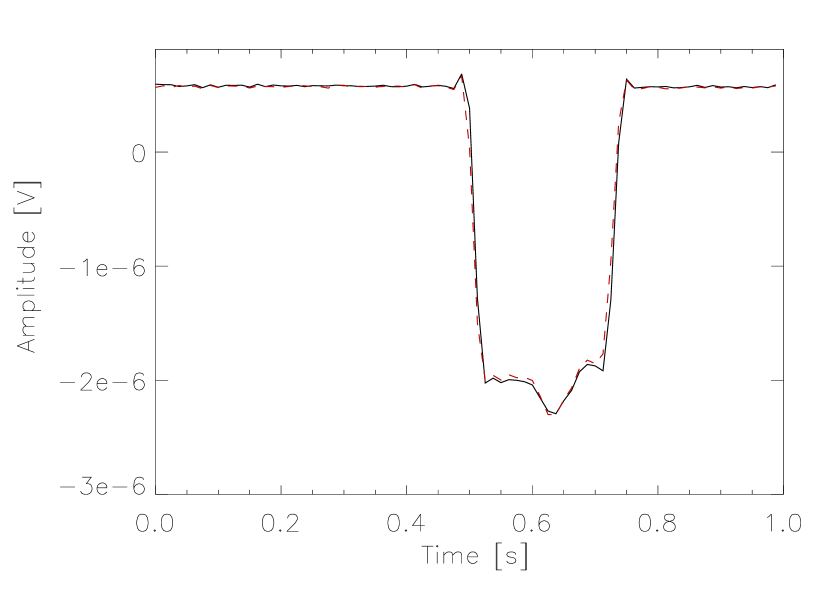
Figure 3 shows the effect of applying Eq.7 with the factor to flight data. The correlated noise in sky and load streams (evident in the two upper plots of the figure) is reduced dramatically. The residual noise has a knee frequencies of 25 mHz, and little effect on maps of the sky, as described in Sect. 7.

3.3 The diode combination
Having two diodes for each radiometer enables observation of both sky and load with a combined duty cycle of almost 100%. In combining the outputs, however, we must take into account the effects of imperfect isolation and differences in noise between the two diodes.
Isolation between diodes was measured for each radiometer in ground tests and verified in flight using the CMB dipole, planets, and Galactic plane crossings. Typical values range from to dB. This is within specifications, and does not compromise LFI sensitivity. It does, however, produce a small anti-correlation of the white noise of the two diodes of a given radiometer. When data from the two diodes are averaged, the white noise of the resulting TOI is lower than would be the case if they were statistically independent. A complete mathematical description of this behaviour is given in Mennella et al. (2011). This causes no difficulty in subsequent calibration and further processing; however, the effect must be taken into account in inferring the noise properties of individual detector chains from the combined outputs.
To take account of differences in noise in combining the diode outputs, we assign relative weights to the uncalibrated diode time-streams based on their calibrated noise. Specifically, we make a first order calibration of the timelines, and , subtract a signal estimate, and calculate the calibrated white noise levels, and , for the two diodes. The weights for the two diodes ( or 1) are
| (8) |
where the weighted calibration constant is given by
| (9) |
and is the same for each diode.
The weights are fixed to a single value per radiometer for the entire dataset. Since all calibrations, noise estimation, and other tests are done on these combined data streams, small errors in the weights cause inconsequential losses in sensitivity, and no systematic errors.
3.4 Detector pointing
Detector pointing is a fundamental ingredient in data processing that requires knowledge of the spacecraft attitude and the location of the horns in the focal plane. The AHF gives the orientation of the spacecraft spin axis in quaternions sampled at 8 Hz, as well as beginning and ending times for a single pointing period. It specifies with appropriate flags the periods of spin-axis maneuvers during which star tracker positions are unreliable. Horn locations within the focal plane are determined from both ground measurements and planet crossings.
The orientation of the spacecraft spin axis at the time of each data sample is determined by linear spherical interpolation of the 8 Hz quaternions. Individual detector pointings are determined by simple rotations from the spin-axis reference frame to the telescope optical axis, then to the relevant horn position, with an additional rotation to account for the orientation of the horn in the focal plane.
In some cases small extrapolations of the quaternions are necessary at the end of a pointing period. Simulations verify that these introduce no significant degradation of the pointing accuracy.
4 Main beams and the geometrical calibration of the focal plane
Knowledge of the beams is of paramount importance in CMB experiments. Errors and uncertainties, and the details of complex non-Gaussian shapes, directly affect cosmological parameters.
We determine the main beam parameters and the position of each horn in the focal plane from planet observations. Jupiter gives the best results, but other planets and bright celestial sources have been used as well. Inputs to the calculations include TOI from each radiometer throughout the planet crossing, the AHF for the same period, and the time-dependent position of the planet as seen by Planck, provided by the JPL Horizons system, which accounts for both spacecraft and planet motion.
4.1 Algorithm and testing
We create a 2D map of the footprint of the focal plane on the sky by selecting data within 10∘ of the telescope line of sight. This comprises the whole extension of the LFI focal plane. To minimize the effects of noise on weak sources, we use TOI from which offsets per ring derived by the Madam destriper (Sect. 7) have already been removed.
We fit a bivariate Gaussian beam model to these data (Burigana et al. 2001):
| (10) | |||||
Here is an overall amplitude. and are Cartesian coordinates, with , the position of the centre of the beam, and and . and are the beamwidth parameters of the elliptical approximation of the beam shape, and the angle is the reconstructed orientation of the beam in the focal plane and is the actual distance (in astronomical units) of the planet.
We tested our technique with simulations using the measured beam patterns together with a detailed model of the Planck telescope. The simulations included the nominal main and far beam patterns, the effects of smearing caused by the motion of the satellite, and pointing uncertainties. Using these simulations of Jupiter crossings (including instrumental noise and complete sky signal), we are able to reconstruct the main beam shape down to dB and to recover the main beam properties at the 1% level or better for all LFI beams. Table 1 reports results for the main beam properties for a sample of the LFI beams. These figures are representative of our expected accuracy for in-flight beam and focal plane reconstruction.
|
||||||||||||||||||||||||||||||||||||||||||||||||||||||||||||||||||||||
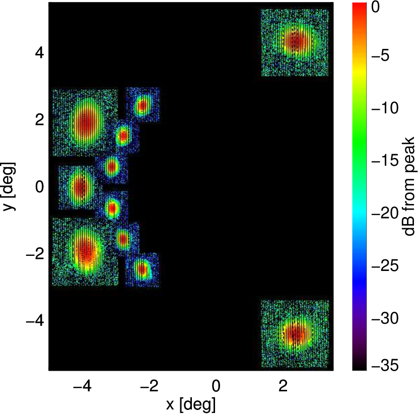
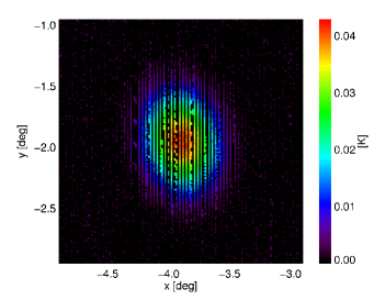
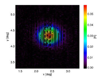
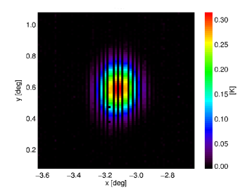
Figure 4 shows the footprint of the LFI focal plane obtained during the first season of Jupiter observations, from 24 October to 1 November 2009. Figure 5 shows beam images for LFI28M, LFI25M and LFI21M from those observations. As expected, all beams are asymmetric but with no significant departures from an elliptical shape visible down to the dB level. For lower levels, aberration starts to distort the beam response, creating non-elliptical shapes.
We also constructed a planet mask, including Jupiter, Mars, and Saturn, the most luminous planets at LFI frequencies. The planet mask is radiometer-dependent, since each horn observes a planet at different times. The planet masking algorithm assigns an appropriate flag to data that lie within an ellipse, centred at the position of the planet and with an orientation that matches the beam orientation, with axes times larger than the beam widths derived from beam fitting. These flags are used in the map-making and ensuing data analysis to discard samples affected by planet transits
5 Photometric calibration
5.1 First steps
The ideal source for photometric calibration, i.e., conversion of the data from volts to kelvin, should be constant, perfectly known, present during all observations, and have the same frequency spectrum as the CMB. In the frequency range of the LFI, the CMB dipole, caused by the motion of the Solar system with respect to the CMB reference frame, satisfies nearly all of these requirements, lacking only in that it is well, but not perfectly, known. The modulation induced on the CMB dipole by the orbital motion of Planck around the Sun satisfies even this last requirement, and will be the ultimate calibration source for the LFI; however, it cannot be used effectively until data for a full orbit of the Sun are available. For this paper, therefore, we must use the CMB dipole. We follow essentially the calibration procedure used for the first year data (Hinshaw et al. 2003). For the pointing period, the signal from each detector can be written as
| (11) |
where is the sky signal, is the noise, and and are the gain and baseline solution. The dominant sky signal on short time scales is the CMB dipole (Galactic plane crossings produce a localized spike that is easy to exclude). This is modeled as
| (12) |
where we have considered both the cosmological dipole and the modulation from the spacecraft motion . We fit for and for each pointing period by minimising
| (13) |
The sum includes unflagged samples within a given pointing period that lie outside a Galactic mask.
The mask is created from simulations of microwave emission provided by the Planck Sky Model (PSM)222The Planck Sky Model is available at:
http://www.apc.univ-paris7.fr/APC_CS/Recherche/Adamis/
PSM/psky-en.html.
Of the LFI frequencies, 30 GHz has the strongest diffuse foreground emission. The mask excludes all pixels that in the 30 GHz PSM are more than times the expected rms of the CMB. It also excludes point sources brighter than 1 Jy found in a compilation of all radio catalogues available at high frequencies (the Planck Input Catalogue, see Massardi 2006). The Galactic and point source masks preserve of the sky.
The Planck scan strategy is such that the instrument field of view describes nearly great circles on the sky. The signal mean is therefore almost zero and nearly constant from one circle to the next. This reduces the correlation between the gain and baseline solutions, a feature also taken advantage of by WMAP (Hinshaw et al. 2003).
As pointed out by Hinshaw et al. (2003) and Cappellini et al. (2003), the largest source of error in Eq. 13 arises from unmodelled sky signal from CMB anisotropy and emission from the Galaxy. To correct this, we solve iteratively for both and . If is the solution at a certain iteration, the next solution is derived using Eq. 13 with
| (14) |
where is the sky signal (minus dipole components) estimated from a sky map built from the previous iteration step. This is repeated to convergence, typically after a few tens of iterations. Figure 6 shows the gain error induced by unmodeled sky signal in a one-year simulation of one 30 GHz detector. The simulation includes CMB anisotropies, the CMB dipole, and Galactic emission. Gain errors in this example are after one iteration. After a few tens of iterations, the residual errors are over the entire year.
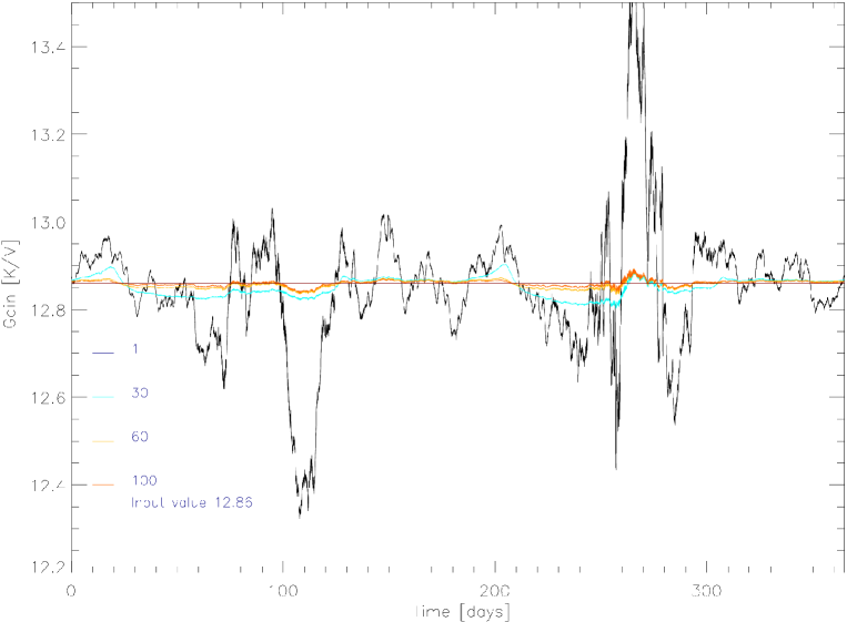
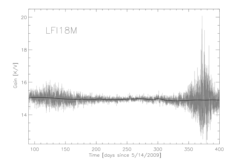
The algorithm alternates between dipole fitting and map-making. Maps are made with (Madam Sect. 7) ignoring polarisation, with no noise prior and baseline length equal to the pointing period length. To improve calibration and reduce noise, calibration is performed simultaneously for both radiometers of each single horn. In the presence of real noise, the actual scatter from one gain solution to the other is quite large. Figure 7 shows an example of the hourly gain solution (grey line) derived from the iterative scheme described above for LFI18M, one of the 70 GHz radiometers. Apart from the scatter induced by instrument noise, the gain solution is quite stable throughout the observation period. Around the dipole maxima, typical noise-induced variations are 0.8% (rms). Nonetheless, the stability of the gain solution is poor compared to the stability of the instrument itself, as indicated by the stability of the uncalibrated white noise level of both differenced and undifferenced data, or the stability of the total power from both sky and load signals. This is particularly evident during the minima of the dipole signal (see Mennella et al. 2011 for further details).
There are also specific things that affect the gain solution. To the extent that they can be measured and understood, their effects on the gain can be corrected directly. For example, a non-linearity in the analogue-to-digital converters (ADCs), discovered during data analysis, produces a multiplicative effect on the data that is recovered (erroneously) by the calibration pipeline as a gain variation. We have developed two independent, complementary methods to correct for this. In the first, we calibrate the data using the gain solution that follows the induced ADC gain variation. In the second, we model the nonlinearity and remove the effect at the raw TOI level.
Alternatively, temperature variations of the amplifiers can induce real gain variations on short time scales. For example, during the first 259 days after launch the downlink transponder was powered up only for downlinks. This induced rather sharp daily variations in the temperature and gain of the amplifiers in the back-end unit (BEM). Starting on day 259, the transponder has been powered up continuously, eliminating this source of gain variations.
In the next section we discuss additional steps taken in the calibration procedure to deal with the effects of noise and gain changes induced by events such as the transponder cycle change.
5.2 Improving calibration accuracy
As shown in Fig. 7, the hourly gain solutions are strongly affected by noise. To reduce the effects of noise and recover more accurately the true and quite stable gains of the instrument, we process the hourly gain solution as follows:
-
•
calculate running averages of length 5 and 30 days. The 5-day averages are still noisy during dipole minima, while the 30-day averages do not follow real but rapid gain changes accurately.
-
•
further smooth the 5- and 30-day curves with wavelets;
-
•
use the 30-day wavelet-smoothed curve during dipole minima;
-
•
use the 5-day unsmoothed curve around day 259 (the downlink transponder change) to trace real gain variations;
-
•
use the 5-day wavelet smoothed curve elsewhere.
A typical gain solution is plotted in Fig. 7 as the solid black line. From the 5- and 30-day gain curves we infer information on the actual gain stability of the instrument as the mission progresses, and also on the overall uncertainty in the gain reconstruction. Specifically, the rms of the over a period of pointings is
| (15) |
where is the average of the gains. The effect of the wavelet smoothing filter is to average over a number of consecutive pointings. Ignoring the different weights in the average, the overall uncertainty can be approximated as
| (16) |
Table 2 lists the largest statistical uncertainties and their associated mean gains out of four time windows (days 100–140, 280–320, 205–245, 349–389, the first two corresponding to minimum and the second two to maximum dipole response), for the main and side arms of the LFI radiometers. In order to provide conservative estimates, we have always chosen a value for corresponding to the number of pointings in 5 days, even in cases where a 30-day smoothing window was used. Equations 15 and 16 and Table 2 are the same as equations 12 and 13 and Table 9 of Mennella et al. (2011). Peak-to-peak variations in the daily gains reach 10% (with mean 7%); however, the rms of the smoothed gain solution is generally in the range. This can be taken as the current level of LFI calibration accuracy.
| Main Arm Side Arm Detector [K/V] [%] [K/V] [%] 70 GHz LFI 18 . 14.935 0.279 22.932 0.243 LFI 19 . 27.434 0.141 41.843 0.228 LFI 20 . 25.572 0.253 29.581 0.261 LFI 21 . 41.629 0.367 41.999 1.038 LFI 22 . 64.275 0.367 62.504 0.185 LFI 23 . 36.492 0.290 54.121 0.382 44 GHz LFI 24 . 282.295 0.349 175.728 0.306 LFI 25 . 123.141 0.358 123.958 0.279 LFI 26 . 167.364 0.398 142.061 0.411 30 GHz LFI 27 . 12.875 0.314 15.320 0.349 LFI 28 . 15.802 0.225 19.225 0.379 |
Although the current pipeline provides results approaching those expected from the stability of the instrument, we are working to improve it as much as possible. In particular, we would like to trace gain variations on time scales shorter than the pointing period. To achieve this, we are developing a detailed gain model (currently under test) based on calibration constants estimated from the pipeline and instrument parameters (temperature sensors, total power data), see Mennella et al. (2011) for further information.
6 Noise estimation
Once data are calibrated, we evaluate the noise properties of each radiometer. We select data in chunks of 5 days each and then compute noise properties. This is done using the roma Iterative Generalized Least Square (IGLS) map-making algorithm (Natoli et al. 2001; de Gasperis et al. 2005) which includes a noise estimation tool based on the iterative approach described in Prunet et al. (2001). IGLS map-making is time and resource intensive and cannot be run over the whole data set within the current DPC system. However since the TOD length considered here is only 5 ODs, it is possible to use the roma implementation of this algorithm which has a noise estimator built-in. The method implemented here is summarized as follows. Model the calibrated TOD as
| (17) |
where is the noise vector, and is a projection matrix that relates a map pixel to a TOD measurement . We obtain a zeroth order estimate of the signal through a rebinned map and then iterate noise and signal estimation:
| (18) |
| (19) |
where is the noise covariance matrix in time domain estimated at iteration . We have verified that convergence is reached in a few, usually three, iterations.
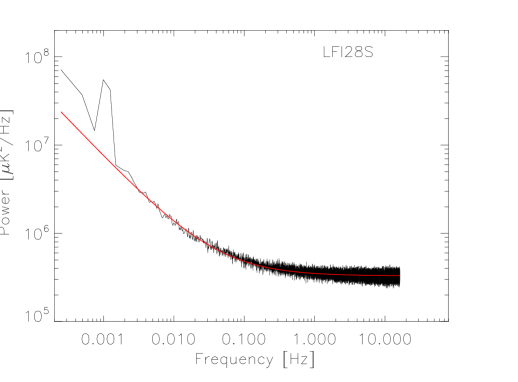
We calculate the Fourier transform of the noise time stream (with an FFT algorithm) and fit the resulting spectrum for the three parameters, the white noise level, the knee-frequency, and the slope of the noise part:
| (20) |
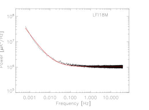
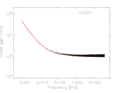
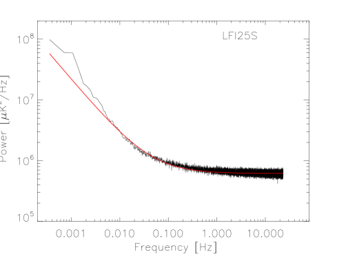
The white noise level is taken as the average of the last few percent of frequency bins. A linear fit to the log-log spectrum low frequency tail gives the slope of the noise. The knee frequency, , is the frequency at which these two straight lines intersect. We tested the accuracy with simulations that included sky signal and instrumental noise with known properties. The noise properties were recovered with typical deviations from input values of for knee-frequency and slope, and less for white noise level. Examples of noise spectra and corresponding fits are shown in Fig. 8.
6.1 Noise constrained realizations and gap filling
The FFT-based noise power spectrum estimation method requires continuity of the noise time stream. As discussed in Sect. 3, we identify bad data (e.g., unstable spacecraft pointing, data saturation effects) and gaps in the data with appropriate flags. We fill in the flagged data with a Gaussian noise realization constrained by data outside the gap (Hoffman & Ribak 1991). Although in principle this method requires a pure noise time stream outside the gap, we have verified that given the low signal-to-noise ratio in the LFI TOD the procedure is not affected by the signal present in the time streams. We fill the gap with Gaussian noise whose properties match those of the noise power spectrum computed over the day immediately before the one with flagged data. An example is shown in Fig. 9.

7 The Map-Making pipeline
7.1 Frequency maps
The map-making pipeline produces sky maps of temperature and polarisation for each frequency channel. It takes as input the calibrated timelines and pointing information in the form of three angles () describing the orientation of the feed horns for each data sample. An essential part of the map-making process is the reduction of correlated noise, a large part which can be removed by exploiting redundancies in the scanning strategy. While the underlying sky signal remains the same, the observed signal varies due to noise. Statistical analysis of the signal variations allows one to distinguish between true sky signals and noise.
Among several map-making codes tested with simulated Planck data (see Ashdown et al. 2007a, b, 2009) the LFI baseline (Mandolesi et al. 2010) is to use the Madam destriping code (Maino et al. 2002). The algorithm and the underlying theory are described in detail in Keihänen et al. (2010); Kurki-Suonio et al. (2009); Keihänen et al. (2005). The basic idea is to model the correlated noise component by a sequence of constant offsets, called baselines. A key parameter in the code is the length of the baseline to be fitted to the data. Madam allows the use of an optional noise prior, if the noise spectrum can be reliably estimated, which further improves the accuracy of the output map. Without the noise prior, the optimal baseline length is of the order of the satellite spin period ( 1 minute). With an accurate noise prior, a much shorter baseline can be used. The shorter the baseline, the closer the Madam solution will be to the optimal Generalized Least Square solution (see Fig. 16 of Ashdown et al. 2009).
We are continually improving our knowledge of the instrument and its noise characteristics, and this information will eventually be used in the Madam algorithm. However, at this stage in the processing we decided to make two simplifications when running our map-making pipeline: no noise prior was used, and all radiometers were weighted equally. These choices lead to a simpler and faster map-making algorithm, which is sufficiently accurate for the Planck Early Results and avoids using detailed parameters describing the instrument which are under continual revision.
With these simplifications, the map-making equations can be written in a concise form. Technically, we are neglecting the baseline covariance, , and setting the white noise variance to unity. The basic model behind the algorithm is
| (21) |
where is the calibrated TOD, is the pointing matrix, is the pixelized sky map, and is the instrumental noise. This last term can be written as
| (22) |
where is the vector of unknown base function amplitudes and the matrix projects these amplitudes into the TOD. Since Madam uses uniform baselines, the matrix consists of ones and zeros, indicating which TOD sample belongs to which baseline. Finally is a pure white noise stream assumed to be statistically independent of the baselines.
The maximum likelihood solution is obtained by minimizing
| (23) |
with respect to the quantities and . The baseline amplitudes are detemined by solving
| (24) |
where
| (25) |
Madam uses an iterative conjugate-gradient method to solve Eq. (24). An estimate for the map is finally obtained as
| (26) |
The map has as many elements as pixels in the sky. Each element is a Stokes parameter triplet for a pixel . The matrix is a 33 block diagonal matrix that operates on map space. There is a block for each pixel . A block can only be inverted if the pixel is sampled with a sufficient number of different polarisation directions to allow determination of the three Stokes parameters for that pixel. This is gauged by the condition number of the block. For the present analysis, if the inverse condition number (ratio of the smallest to largest eigenvalue) was less than 0.01, the pixel was excluded from the map.
The blocks must be inverted when Eqs. (24) and (25) are solved for the baselines. These inversions are computed by eigenvalue decomposition. Eigenvalues whose magnitudes are less than 10-6 times the largest eigenvalue are discarded; only the remaining part is inverted.
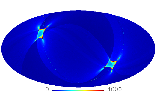
For the present analysis, we need only the -component maps at the three LFI nominal frequencies, combining observations of all radiometers at a given frequency. Figure 10 shows (left column) the hit count maps by frequency. In addition, we produce maps from horn pairs scanning the same path in the sky (see Mennella et al. 2011, for details on the LFI focal plane arrangement). We have produced 30 GHz maps at HEALPix resolution = 512, and 44 and 70 GHz maps at = 1024. All maps are in the NESTED scheme, in Galactic coordinates, with units of thermodynamic kelvin. The baseline length in Madam was one minute333One minute baselines for 30 GHz, 44 GHz, and 70 GHz are 1950, 2792, and 4726 samples respectively..
7.2 White noise covariance matrices
If we bin the pure white noise stream to a map using the pointing , we obtain a binned white noise map,
| (27) |
This map is a theoretical concept because we do not have access to the radiometer white noise streams. Its covariance matrix, however, is important because it provides an estimate of both the white noise power in each pixel and white noise correlations between Stokes parameters at a given pixel.
This white noise covariance matrix (WNC) is computed as (Eq. 27)
| (28) |
Here , is a matrix that operates in the TOD domain, and angle brackets denote the ensemble mean. Because the radiometers have independent white noise, is diagonal. We assume that each radiometer has a uniform white noise variance (see Sect. 6), but that each radiometer has its own variance. The radiometer values that we used in the WNC computation are reported in Mennella et al. (2011).
7.3 Half-ring jackknife noise maps
For noise estimation purposes we divided the time ordered data into two halves and produced jackknife maps as follows. Each pointing period lasts typically 44 min (median 43.5 min, standard deviation 10 min). Typically, during the first 4 min the pointing is unstable, so these data are not used for science. During the remaining stable 40 min, each horn scans a ring on the sky. This ring consists of scan circles. One full scan circle takes 1 min. Therefore, each ring has about 40 scan circles. We made half-ring jackknife maps (and ) with the same pipeline as described in Sect. 7.1, but using stable data only from the first or the second half of each pointing period. Specificaly, this is implemented by marking the other half of each ring as a gap in the data. Madam knows that for any given pointing period the first-used scan circle/sample of any half-ring is far apart in time (typically 25 min) from the last used scan circle/sample of the previous half-ring.
At each pixel , the jackknife maps and contain the same sky signal (as long no time-varying sources or moving objects cross at the time of observation), since they result from the same scanning pattern on the sky. However, because of instrumental noise, the maps and are not identical.
We can estimate the sky signal+noise as
| (29) |
and the noise in map as
| (30) |
This noise map includes noise that is not correlated on timescales longer than 20 minutes. In particular, gives a good estimate of the white noise in .
However, we are interested in the noise level in the full map , (see Eq. 26). To estimate this, we construct another noise map
| (31) |
with weights
| (32) |
Here is the hit count at pixel in the full map , while and are the hit counts of and , respectively. The weight factor is equal to only in those pixels where . In a typical pixel, will differ slightly from and hence the weight factor is .
7.4 Noise Monte Carlo simulations
To check the noise analysis, we produced Monte Carlo noise realizations on the “Louhi” supercomputer at “CSC-IT Center for Science” in Finland. The simulation takes as input estimates of the white noise , knee frequency, and slope of the noise estimated from the TOD for each radiometer (Mennella et al. 2011), as well as satellite pointing information. Flight pointing was reconstructed to machine accuracy using Planck Level-S simulation software Reinecke et al. (2006). For each frequency channel, we generated 101 Monte Carlo realizations of the noise, simulating white noise and correlated noise () streams separately. Maps from these noise streams were produced with the map-making pipeline described in Sect. 7.1. For each simulated noise map, we computed the corresponding binned white noise maps defined in Eq. (27). The production of the binned white noise maps allows us to study the residual correlated noise, i.e., the difference between the total and binned white noise maps Kurki-Suonio et al. (2009). These Monte Carlo simulations were used to test and validate several approaches to noise estimation described in detail in the LFI instrument paper (Mennella et al. 2011).
8 Colour correction
The power measured by LFI can be expressed as
| (33) |
where is the overall gain, is the bandpass, and is the Rayleigh-Jeans brightness temperature signal, in the case of LFI calibration procedure, due to the CMB dipole. At a given frequency , the overall gain is equal to . For small fluctuations around the mean CMB temperature , the relation between intensity, , Rayleigh-Jeans brightness temperature , and thermodynamic temperature is
| (34) |
The differential black-body spectrum is
| (35) |
| (36) |
The function is the differential black-body spectrum in Rayleigh-Jeans units. With our definition of the overall gain , the bandpasses are normalised such that
| (37) |
Calibration data provide a nominal brightness temperature ; however, this is only exact for a monochromatic response. For a non-zero bandwidth, a colour correction is required to convert the brightness temperature for emission with a particular spectral index to that of the map:
| (38) |
By definition, the colour correction is unity when the source observed has a CMB spectrum. Within each LFI band, is well-approximated by a power law with spectral index .
The general expression for the colour correction is
| (39) |
where we assumed a power-law spectrum with temperature spectral index . The term in square brackets is unity with our normalisation for , but has been included to show that depends only on the shape and not the amplitude of the bandpass. Thus is independent of .
Each detector has a different bandpass, hence its own colour correction. We derive approximate colour corrections for band-averaged sky maps using bandpasses averaged over: (i) the two detectors in each radiometer; (ii) the two orthogonally-polarised radiometers behind each feed horn; and (iii) the several feed horns in each frequency band. In addition, although the bandpass is mainly defined by the front-end (Bersanelli et al. 2010), differences between back-end bandpasses on a single radiometer are measurable, e.g., in the form of -dependent residuals in difference images.
Since the current sky maps have been produced, both for pairs of horns and for several horns in each band, with calibrated data combined with equal weights, we have used an unweighted average of all the contributing bandpasses for our band-averaged corrections. Using the bandpass models given in Zonca et al. (2009) derived from the pre-launch calibration campaign, we evaluate the integrals in Eq.(39) analytically for several spectral indices. The results are given in Table 3.
|
||||||||||||||||||||||||||||||||||||||||||||||||||||||||||||||||||||||||||||||||||||||||||||||||||||||||||||||||||||||||||||||||||||||||||||||||||||||||||
At the current stage of the mission and data analysis, uncertainties in the colour corrections are much smaller than those of the gains ; however we aim to reduce the calibration error (using the orbital dipole) to below 0.2%. Two primary sources of error in will then need to be considered. The first is related to uncertainties in the bandpass model (Leahy et al. 2010; Zonca et al. 2009). The second arises from the uneven sampling of individual sky pixels by the full set of detectors, which causes pixel-to-pixel variations in the colour correction.
9 CMB removal
This section was developed in common with HFI (Planck HFI Core Team 2011b) and is reported identically in both papers.
In order to facilitate foreground studies with the frequency maps, a set of maps was constructed with an estimate of the CMB contribution subtracted from them. The steps undertaken in determining that estimate of the CMB map, subtracting it from the frequency maps, and characterising the errors in the subtraction are described below.
9.1 Masks
Point source masks were constructed from the source catalogues produced by the LFI pipeline for each of the LFI frequency channel maps. The algorithm used in the pipeline to detect the sources was a Mexican-hat wavelet filter. All sources detected with a signal-to-noise ratio greater than 5 were masked with a cut of radius of the effective beam. A similar process was applied to the HFI frequency maps (Planck HFI Core Team 2011b).
Galactic masks were constructed from the 30 GHz and 353 GHz frequency channel maps. An estimate of the CMB was subtracted from the maps in order not to bias the construction. The maps were smoothed to a common resolution of 5∘. The pixels within each mask were chosen to be those with values above a threshold value. The threshold values were chosen to produce masks with the desired fraction of the sky remaining. The point source and Galactic masks were provided as additional inputs to the component separation algorithms.
9.2 Selection of the CMB template
Six component separation or foreground removal algorithms were applied to the HFI and LFI frequency channel maps to produce CMB maps. They are, in alphabetical order:
-
•
AltICA: Internal linear combination (ILC) in the map domain;
-
•
CCA: Bayesian component separation in the map domain;
-
•
FastMEM: Bayesian component separation in the harmonic domain;
-
•
Needlet ILC: ILC in the needlet (wavelet) domain;
-
•
SEVEM: Template fitting in map or wavelet domain;
-
•
Wi-fit: Template fitting in wavelet domain.
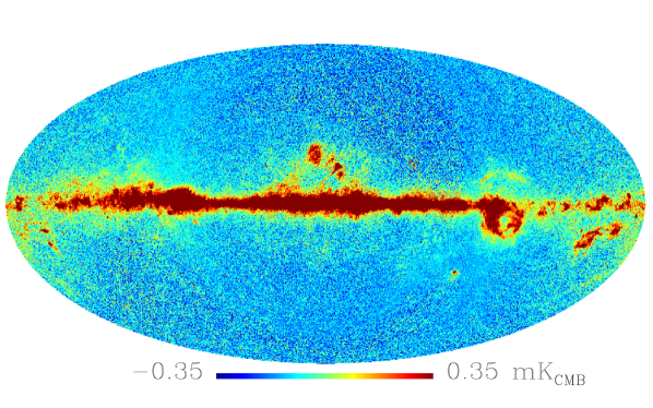
Details of these methods may be found in Leach et al. (2008). These six algorithms make different assumptions about the data, and may use different combinations of frequency channels used as input. Comparing results from these methods (see Fig. 14) demonstrated the consistency of the CMB template and provided an estimate of the uncertainties in the reconstruction. A detailed comparison of the output of these methods, largely based on the CMB angular power spectrum, was used to select the CMB template that was removed from the frequency channel maps. The comparison was quantified using a jackknife procedure: each algorithm was applied to two additional sets of frequency maps made from the first half and second half of each pointing period. A residual map consisting of half the difference between the two reconstructed CMB maps was taken to be indicative of the noise level in the reconstruction from the full data set. The Needlet ILC (hereafter NILC) map was chosen as the CMB template because it had the lowest noise level at small scales.
The CMB template was removed from the frequency channel maps after application of a filter in the spherical harmonic domain. The filter has a transfer function made of two factors. The first corresponds to the Gaussian beam of the channel to be cleaned; the second is a transfer function attenuating the multipoles of the CMB template that have low signal-to-noise ratio. It is designed in Wiener-like fashion, being close to unity up to multipoles around , then dropping smoothly to zero with a cut-off frequency around (see Fig. 11). All angular frequencies above are completely suppressed.
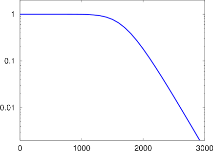
This procedure was adopted to avoid doing more harm than good to the small scales of the frequency channel maps where the signal-to-noise ratio of the CMB is low.
9.3 Description of Needlet ILC
The NILC map was produced using the ILC method in the “needlet” domain. Needlets are spherical wavelets that allow localisation both in multipole and sky direction. The input maps are decomposed into twelve overlapping multipole domains (called “scales”), using the bandpass filters shown in Fig. 12
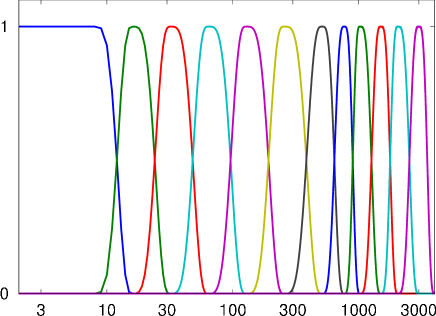
and further decomposed into regions of the sky. Independent ILCs are applied in each sky region at each needlet scale. Large regions are used at large scales, while smaller regions are used at fine scales.
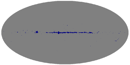
The NILC template was produced from all six HFI channels, using the tight Galactic mask shown in figure 13, which covers 99.36% of the sky. Additional areas are excluded on a per-channel basis to mask point sources. Future inclusion of the LFI channels will improve cleaning of low-frequency foregrounds such as synchrotron emission from the CMB template.
Before applying NILC, pixels missing due to point source and Galactic masking are filled in by a “diffusive inpainting” technique, which consists of replacing each missing pixel by the average of its neighbours and iterating to convergence. This is similar to solving the heat diffusion equation in the masked areas with boundary conditions given by the available pixel values at the borders of the mask. All maps are re-beamed to a common resolution of 5′. Re-beaming blows up the noise in the less resolved channels, but that effect is automatically taken into account by the ILC filter.
9.4 Uncertainties in the CMB removal
The uncertainties in the CMB removal have been gauged in two ways, firstly by comparing the CMB maps produced by the different algorithms and secondly by applying the NILC coefficients to jackknife maps.
9.4.1 Dispersion of the CMB maps produced by the various algorithms.
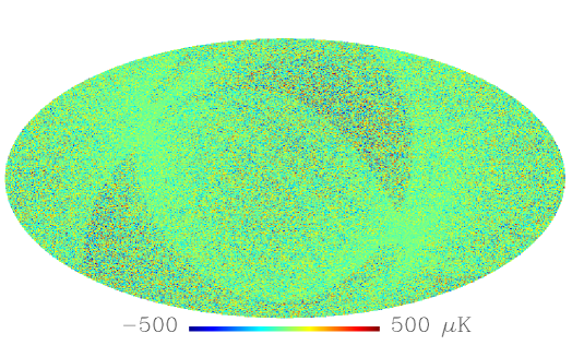
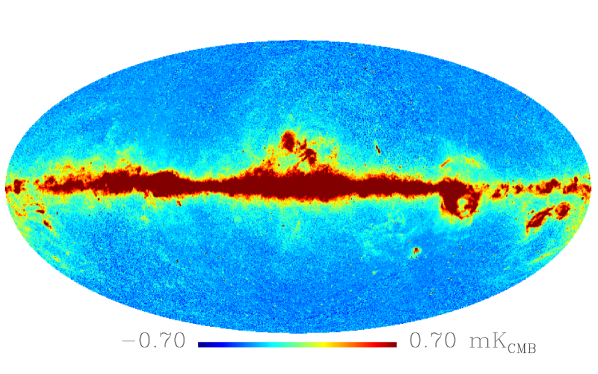
The methods that were used to produce the estimates of the CMB are diverse. They work by applying different algorithms (ILC, template fitting, or Bayesian parameter estimation) in a variety of domains (pixel space, Needlet/wavelet space, or spherical harmonic coefficients). Each method carries out its optimisation in a different way and thus will respond to the foregrounds differently. Dispersion in the CMB rendition by different methods provides an estimate of the uncertainties in the determination of the CMB, and thus in the subtraction process. The rms difference between the NILC map and the other CMB estimates is shown in Fig. 14. As expected, the uncertainties are largest in the Galactic plane where the foregrounds to remove are strongest, and smallest around the Ecliptic poles where the noise levels are lowest.
9.4.2 CMB map uncertainties estimated by applying NILC filtering of jackknifes
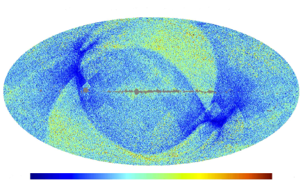
The cleanliness of the CMB template produced by the NILC filter can be estimated using jackknives. We apply the NILC filter to the maps built from the first and last halves of the ring set. The power distribution of the half-difference of the results provides us with a reliable estimate of the power of the noise in the NILC CMB template, (while previous results correspond to applying the NILC filter to the half-sum maps from which they can be derived).
The jackknives allow estimates of the relative contributions of sky signal and noise to the total data power. Assume that the data are in the form where is the sky signal and is the noise, independent of . The total data power decomposes as . One can obtain by applying the NILC filter to half difference maps, and follows from . This procedure can be applied in pixel space, in harmonic space, or in pixel space after the maps have been bandpass-filtered, as described next.
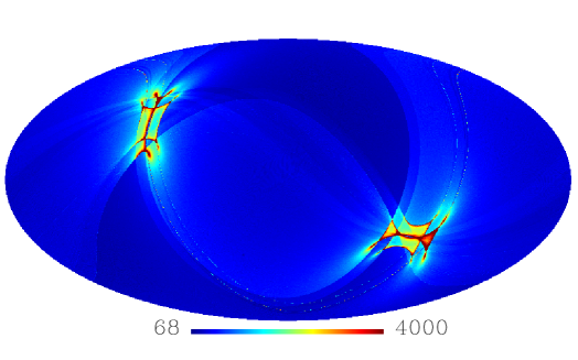
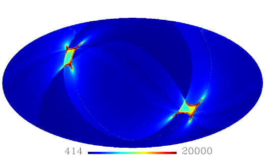
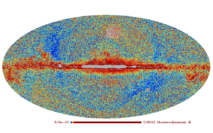
We first used pixel space jackknifing to estimate the spatial distribution of noise. Figure 15 shows a map of the local rms of the noise. We applied the NILC filter to a half-difference map and we display the square root of its smoothed squared values, effectively resulting in an estimate of the local noise rms.
Using the same approach, we obtain an estimate of the angular spectrum of the noise in the NILC map, shown in Fig 16. That spectrum corresponds to an rms of 11 K per pixel.
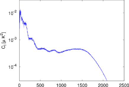
The “features” in the shape of the noise angular spectrum at large scale are a consequence of the needlet-based filtering (such features would not appear in a pixel-based ILC map). Recall that the coefficients of an ILC map are adjusted to minimize the total contamination by both foregrounds and noise. The strength of foregrounds relative to noise being larger at coarse scales, the needlet-based ILC tends to let more noise in, with the benefit of better foreground rejection.
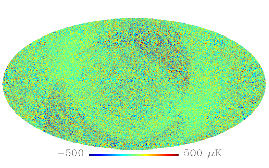
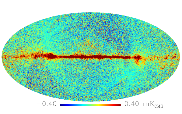
The half-difference maps offer simple access to the power distribution of the residual noise in the estimated CMB template. However, it is more difficult to evaluate other residual contamination, since all fixed sky emissions cancel in half difference maps. Any such large-scale contamination is barely visible in the CMB template, since it is dominated by the CMB itself. However, contamination is more conspicuous if one looks at intermediate scales. Figure 17
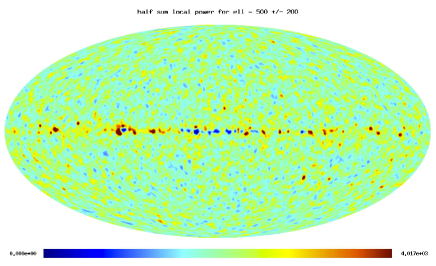
shows the local power of the CMB template after it is bandpassed to retain only multipoles in the range . This smooth version of the square of a bandpassed map clearly shows where the errors in the component separation become large and so complicate some specific science analyses.
10 Infrastructure overview
To organize the large number of data processing codes and data products, the DPC employs the Planck Integrated Data and Information System (IDIS). This allows flexible development of the processing pipeline, while ensuring complete traceability and reproducibility of data products. For this, the most relevant components of IDIS are the Data Management Component (DMC) and the Process Coordinator (ProC), developed at the MPA Planck Analysis Centre (MPAC) at the Max-Planck-Institute for Astrophysics in Garching. Access to both components as well as to the Planck document and software management system is controlled via another IDIS component: the Federation Layer developed and maintained at the ESA ESTEC Research and Scientific Support Department (RSSD).
Here we describe the essential features of the IDIS data processing components and their use at the DPC. A more detailed description of these components and their capabilities will be given in a future paper.
10.1 Data Management Component
The DMC organizes the storage and access to DPC data products. To combine optimal performance in data I/O with the data management capabilities of modern databases, scientific data are stored in files, while metadata identifying them are stored in a database. The data files can only be modified in synchronization with the database, preventing concurrent access to data objects via locking mechanisms. The DMC software supports several database management systems of various complexity; the LFI DPC operates an Oracle 10g database, which ensures good performance and stability.
The DMC provides a uniform Application Programming Interface (API) for Fortran, C, C++, and Java, hiding all specific database operations from the user, who is therefore not required to have database experience. DMC data types are defined in the Data Definition Layer (DDL), which describes data and metadata structures. The DDL supports inheritance of data types (e.g., a data type polarized_map can be inherited from a data type map) as well as association of data types (i.e., one data type containing a reference to another).
In addition to the API, the DMC provides a Graphical User Interface (GUI), which supports user queries of the database and retrieval of information on the data. The GUI offers the user the ability to list the (meta-)data of specific objects and also to visualize the data in a simple way (although data can also be exported to other powerful visualizing tools). The GUI also allows the display of history information on data objects, permitting the user to browse intermediate data products used in generating those objects, and the controlled deletion of data, observing dependencies of data types and maintaining the history information for all remaining data. For this, the DMC relies on additional metadata on the processing history of the data objects, which are generated by the Process Coordinator workflow engine (ProC).
10.2 Pipeline management — the ProC workflow engine
The ProC is a generic engine to construct, verify, and execute computational workflows. It comprises computing modules and data flows between them. The modules can be written in any programming language, provided they conform to simple I/O format requirements described in an XML module description file. These interface files specify the input and output objects, as well as the parameters of the individual programs, in terms of DMC data types as described above.
The ProC provides a Pipeline Editor to support graphical construction of data processing workflows. It allows users to arrange and connect computing modules of a workflow in a clearly structured manner, and at the same time to configure the parameters of the algorithms used. It provides control structures for data flow, for data object I/O and consistent parameter definition.
The execution of workflows is controlled by a forward chaining algorithm, which ensures that modules are executed as soon as all necessary data products and parameters are known. If the same version of a module has been executed with identical inputs and parameters, the ProC will skip the execution and use the data product from the earlier execution for further processing. The ProC maintains control of pipeline execution also on massive parallel computing environments. In the LFI implementation, the ProC communicates with the PBS (Portable Batch System) scheduling system to send jobs to the DPC cluster and to log their execution status.
The ProC logs workflow executions on log files, which can also contain logging messages of the executed modules. Additionally, it creates so-called Pipeline-Run and Module-Run objects in the DMC, which are used to recover the generation history of data products (including versions of processing modules via MD5-sums). Besides the GUI, the ProC can also be executed from the command line.
At the LFI DPC, the ProC is used to execute the official pipeline producing Planck data products.
11 Discussion and conclusions
We have described the status of the pipeline as it stands at the time of the ERCSC release and submission of the Planck early papers. All the algorithms run during this process have been verified, validated, and tested before launch and the start of operations using realistic simulations. This allowed us to begin analyzing the data as soon as they were acquired from the first day of operations. The entire Level 1 pipeline suffered no significant problems, and all of the data were transformed efficiently from telemetry packets to timelines. At present, the Level 2 pipeline is capable of providing relative calibration to an overall statistical accuracy in the range 0.05–0.1% and absolute calibration at around the 1% level. The beams are accurately characterised down to dB. We expect to improve many aspects in the near future. Concerning the calibration, our intention is to reach the levels determined by the stability of the instrument. For the beam reconstruction, our aim is to improve the characterisation of the far side lobes and to refine the entire beam reconstruction pipeline, with particular attention to polarization measurements.
Acknowledgements.
Planck is too large a project to allow full acknowledgement of all contributions by individuals, institutions, industries, and funding agencies. The main entities involved in the mission operations are as follows. The European Space Agency operates the satellite via its Mission Operations Centre located at ESOC (Darmstadt, Germany) and coordinates scientific operations via the Planck Science Office located at ESAC (Madrid, Spain). Two Consortia, comprising around 50 scientific institutes within Europe, the USA, and Canada, and funded by agencies from the participating countries, developed the scientific instruments LFI and HFI, and continue to operate them via Instrument Operations Teams located in Trieste (Italy) and Orsay (France). The Consortia are also responsible for scientific processing of the acquired data. The Consortia are led by the Principal Investigators: J.L. Puget in France for HFI (funded principally by CNES and CNRS/INSU-IN2P3) and N. Mandolesi in Italy for LFI(funded principally via ASI). NASA US Planck Project, based at JPL and involving scientists at many US institutions, contributes significantly to the efforts of these two Consortia. The author list for this paper has been selected by the Planck Science Team, and is composed of individuals from all of the above entities who have made multi-year contributions to the development of the mission. It does not pretend to be inclusive of all contributions. The Planck-LFI project is developed by an International Consortium lead by Italy and involving Canada, Finland, Germany, Norway, Spain, Switzerland, UK, USA. The Italian contribution to Planck is supported by the Italian Space Agency (ASI) and INAF. This work was supported by the Academy of Finland grants 121703 and 121962. We thank the DEISA Consortium (www.deisa.eu), co-funded through the EU FP6 project RI-031513 and the FP7 project RI-222919, for support within the DEISA Virtual Community Support Initiative. We thank CSC – IT Center for Science Ltd (Finland) for computational resources. We acknowledge financial support provided by the Spanish Ministerio de Ciencia e Innovaciõn through the Plan Nacional del Espacio y Plan Nacional de Astronomia y Astrofisica. We acknowledge The Max Planck Institute for Astrophysics Planck Analysis Centre (MPAC) is funded by the Space Agency of the German Aerospace Center (DLR) under grant 50OP0901 with resources of the German Federal Ministry of Economics and Technology, and by the Max Planck Society. This work has made use of the Planck satellite simulation package (Level-S), which is assembled by the Max Planck Institute for Astrophysics Planck Analysis Centre (MPAC) Reinecke et al. (2006). We acknowledge financial support provided by the National Energy Research Scientific Computing Center, which is supported by the Office of Science of the U.S. Department of Energy under Contract No. DE-AC02-05CH11231. Some of the results in this paper have been derived using the HEALPix package Górski et al. (2005). A description of the Planck Collaboration and a list of its members, indicating which technical or scientific activities they have been involved in, can be found at http://www.rssd.esa.int/index.php?project=PLANCK&page=Planck_Collaboration.References
- Ashdown et al. (2007a) Ashdown, M. A. J., Baccigalupi, C., Balbi, A., et al. 2007a, A&A, 471, 361
- Ashdown et al. (2007b) Ashdown, M. A. J., Baccigalupi, C., Balbi, A., et al. 2007b, A&A, 467, 761
- Ashdown et al. (2009) Ashdown, M. A. J., Baccigalupi, C., Bartlett, J. G., et al. 2009, A&A, 493, 753
- Bersanelli et al. (2010) Bersanelli, M., Mandolesi, N., Butler, R. C., et al. 2010, A&A, 520, A4+
- Burigana et al. (2001) Burigana, C., Natoli, P., Vittorio, N., Mandolesi, N., & Bersanelli, M. 2001, Experimental Astronomy, 12, 87, 10.1023/A:1016338603042
- Cappellini et al. (2003) Cappellini, B., Maino, D., Albetti, G., et al. 2003, A&A, 409, 375
- de Gasperis et al. (2005) de Gasperis, G., Balbi, A., Cabella, P., Natoli, P., & Vittorio, N. 2005, A&A, 436, 1159
- Frailis et al. (2009) Frailis, M., Maris, M., Zacchei, A., et al. 2009, Journal of Instrumentation, 4, 2021
- Górski et al. (2005) Górski, K. M., Hivon, E., Banday, A. J., et al. 2005, ApJ, 622, 759
- Hinshaw et al. (2003) Hinshaw, G., Spergel, D. N., Verde, L., et al. 2003, ApJS, 148, 135
- Hoffman & Ribak (1991) Hoffman, Y. & Ribak, E. 1991, ApJ, 380, L5
- Keihänen et al. (2010) Keihänen, E., Keskitalo, R., Kurki-Suonio, H., Poutanen, T., & Sirviö, A. 2010, A&A, 510, A57+
- Keihänen et al. (2005) Keihänen, E., Kurki-Suonio, H., & Poutanen, T. 2005, MNRAS, 360, 390
- Kurki-Suonio et al. (2009) Kurki-Suonio, H., Keihänen, E., Keskitalo, R., et al. 2009, A&A, 506, 1511
- Lamarre et al. (2010) Lamarre, J., Puget, J., Ade, P. A. R., et al. 2010, A&A, 520, A9+
- Leach et al. (2008) Leach, S. M., Cardoso, J., Baccigalupi, C., et al. 2008, A&A, 491, 597
- Leahy et al. (2010) Leahy, J. P., Bersanelli, M., D’Arcangelo, O., et al. 2010, A&A, 520, A8+
- Maino et al. (2002) Maino, D., Burigana, C., Górski, K. M., Mandolesi, N., & Bersanelli, M. 2002, A&A, 387, 356
- Mandolesi et al. (2010) Mandolesi, N., Bersanelli, M., Butler, R. C., et al. 2010, A&A, 520, A3+
- Maris et al. (2009) Maris, M., Tomasi, M., Galeotta, S., et al. 2009, Journal of Instrumentation, 4, 2018
- Massardi (2006) Massardi, M. 2006, in CMB and Physics of the Early Universe
- Meinhold et al. (2009) Meinhold, P., Leonardi, R., Aja, B., et al. 2009, Journal of Instrumentation, 4, 2009
- Mennella et al. (2010) Mennella, A., Bersanelli, M., Butler, R. C., et al. 2010, A&A, 520, A5+
- Mennella et al. (2003) Mennella, A., Bersanelli, M., Seiffert, M., et al. 2003, A&A, 410, 1089
- Mennella et al. (2011) Mennella et al. 2011, Planck early results 03: First assessment of the Low Frequency Instrument in-flight performance (Submitted to A&A, [arXiv:astro-ph/1101.2038])
- Natoli et al. (2001) Natoli, P., de Gasperis, G., Gheller, C., & Vittorio, N. 2001, A&A, 372, 346
- Pasian & Gispert (2000) Pasian, F. & Gispert, R. 2000, Astrophysical Letters Communications, 37, 247
- Planck Collaboration (2011a) Planck Collaboration. 2011a, Planck early results 01: The Planck mission (Submitted to A&A, [arXiv:astro-ph/1101.2022])
- Planck Collaboration (2011b) Planck Collaboration. 2011b, Planck early results 02: The thermal performance of Planck (Submitted to A&A, [arXiv:astro-ph/1101.2023])
- Planck Collaboration (2011c) Planck Collaboration. 2011c, Planck early results 07: The Early Release Compact Source Catalogue (Submitted to A&A, [arXiv:astro-ph/1101.2041])
- Planck Collaboration (2011d) Planck Collaboration. 2011d, Planck early results 08: The all-sky early Sunyaev-Zeldovich cluster sample (Submitted to A&A, [arXiv:astro-ph/1101.2024])
- Planck Collaboration (2011e) Planck Collaboration. 2011e, Planck early results 09: XMM-Newton follow-up for validation of Planck cluster candidates (Submitted to A&A, [arXiv:astro-ph/1101.2025])
- Planck Collaboration (2011f) Planck Collaboration. 2011f, Planck early results 10: Statistical analysis of Sunyaev-Zeldovich scaling relations for X-ray galaxy clusters (Submitted to A&A, [arXiv:astro-ph/1101.2043])
- Planck Collaboration (2011g) Planck Collaboration. 2011g, Planck early results 11: Calibration of the local galaxy cluster Sunyaev-Zeldovich scaling relations (Submitted to A&A, [arXiv:astro-ph/1101.2026])
- Planck Collaboration (2011h) Planck Collaboration. 2011h, Planck early results 12: Cluster Sunyaev-Zeldovich optical Scaling relations (Submitted to A&A, [arXiv:astro-ph/1101.2027])
- Planck Collaboration (2011i) Planck Collaboration. 2011i, Planck early results 13: Statistical properties of extragalactic radio sources in the Planck Early Release Compact Source Catalogue (Submitted to A&A, [arXiv:astro-ph/1101.2044])
- Planck Collaboration (2011j) Planck Collaboration. 2011j, Planck early results 14: Early Release Compact Source Catalogue validation and extreme radio sources (Submitted to A&A, [arXiv:astro-ph/1101.1721])
- Planck Collaboration (2011k) Planck Collaboration. 2011k, Planck early results 15: Spectral energy distributions and radio continuum spectra of northern extragalactic radio sources (Submitted to A&A, [arXiv:astro-ph/1101.2047])
- Planck Collaboration (2011l) Planck Collaboration. 2011l, Planck early results 16: The Planck view of nearby galaxies (Submitted to A&A, [arXiv:astro-ph/1101.2045])
- Planck Collaboration (2011m) Planck Collaboration. 2011m, Planck early results 17: Origin of the submillimetre excess dust emission in the Magellanic Clouds (Submitted to A&A, [arXiv:astro-ph/1101.2046])
- Planck Collaboration (2011n) Planck Collaboration. 2011n, Planck early results 18: The power spectrum of cosmic infrared background anisotropies (Submitted to A&A, [arXiv:astro-ph/1101.2028])
- Planck Collaboration (2011o) Planck Collaboration. 2011o, Planck early results 19: All-sky temperature and dust optical depth from Planck and IRAS — constraints on the “dark gas” in our Galaxy (Submitted to A&A, [arXiv:astro-ph/1101.2029])
- Planck Collaboration (2011p) Planck Collaboration. 2011p, Planck early results 20: New light on anomalous microwave emission from spinning dust grains (Submitted to A&A, [arXiv:astro-ph/1101.2031])
- Planck Collaboration (2011q) Planck Collaboration. 2011q, Planck early results 21: Properties of the interstellar medium in the Galactic plane (Submitted to A&A, [arXiv:astro-ph/1101.2032])
- Planck Collaboration (2011r) Planck Collaboration. 2011r, Planck early results 22: The submillimetre properties of a sample of Galactic cold clumps (Submitted to A&A, [arXiv:astro-ph/1101.2034])
- Planck Collaboration (2011s) Planck Collaboration. 2011s, Planck early results 23: The Galactic cold core population revealed by the first all-sky survey (Submitted to A&A, [arXiv:astro-ph/1101.2035])
- Planck Collaboration (2011t) Planck Collaboration. 2011t, Planck early results 24: Dust in the diffuse interstellar medium and the Galactic halo (Submitted to A&A, [arXiv:astro-ph/1101.2036])
- Planck Collaboration (2011u) Planck Collaboration. 2011u, Planck early results 25: Thermal dust in nearby molecular clouds (Submitted to A&A, [arXiv:astro-ph/1101.2037])
- Planck Collaboration (2011v) Planck Collaboration. 2011v, The Explanatory Supplement to the Planck Early Release Compact Source Catalogue (ESA)
- Planck HFI Core Team (2011a) Planck HFI Core Team. 2011a, Planck early results 04: First assessment of the High Frequency Instrument in-flight performance (Submitted to A&A, [arXiv:astro-ph/1101.2039])
- Planck HFI Core Team (2011b) Planck HFI Core Team. 2011b, Planck early results 06: The High Frequency Instrument data processing (Submitted to A&A, [arXiv:astro-ph/1101.2048])
- Prunet et al. (2001) Prunet, S., Ade, P. A. R., Bock, J. J., et al. 2001, ArXiv Astrophysics e-prints
- Reinecke et al. (2006) Reinecke, M., Dolag, K., Hell, R., Bartelmann, M., & Enßlin, T. A. 2006, A&A, 445, 373
- Rosset et al. (2010) Rosset, C., Tristram, M., Ponthieu, N., et al. 2010, A&A, 520, A13+
- Tauber et al. (2010) Tauber, J. A., Mandolesi, N., Puget, J., et al. 2010, A&A, 520, A1+
- Zacchei et al. (2009) Zacchei, A., Frailis, M., Maris, M., et al. 2009, Journal of Instrumentation, 4, 2019
- Zacchei et al. (2011) Zacchei et al. 2011, Planck early results 05: The Low Frequency Instrument data processing (Submitted to A&A, [arXiv:astro-ph/1101.2040])
- Zonca et al. (2009) Zonca, A., Franceschet, C., Battaglia, P., et al. 2009, Journal of Instrumentation, 4, 2010