Application of the Wang–Landau method to faceting phase transition.

Abstract

A simple solid–on–solid model of adsorbate – induced faceting is studied by using a modified Wang–Landau method. The phase diagram for this system is constructed by computing the density of states in a special two–dimensional energy space. A finite–size scaling analysis of transition temperature and specific heat shows that faceting transition is the first order phase transition. Logarithmic dependence of the mean–square width of the surface on system size indicates that surface is rough above the transition temperature.

I Introduction

It has been recently demonstrated song95 ; mad96 ; mad99a ; mad99b ; song07 that surfaces such as W(111) and Mo(111) covered with a single physical monolayer of certain metals (Pd, Rh, Ir, Pt, Au) undergo massive reconstruction from a planar morphology to a faceted surface upon annealing at $T>700$K. The faceted surface is covered by three–sided pyramids with mainly {211} facets. A major mechanism for facets formation is minimization of total surface free energyleung97 . Faceting of bcc(111) and fcc(210) surfaces can also be induced by oxygen or other nonmetallic impurities (see Ref.mad08 and references therein). Adsorbate – induced faceting is also observed on curved surfaces tsong01 ; szczep05 ; szczep05b and this phenomenon has been recently used in fabrication of electron and ion point sources tsong08 ; tsong09 .

Investigations of thermal stability of faceted surfaces have revealed that reversible phase transition occurs in systems Pd/Mo(111)song95 , O/Mo(111)song95 , and Pd/W(111)song07 . As a result of faceting transition, the faceted surface changes into planar surface at the transition temperature.

In theoretical studies of complicated surface problems (e.g. roughening transition, surface reconstruction, surface growth, surface phase transitions) simple models like lattice gas models or solid–on–solid (SOS) models are applied beijeren95 ; tosat96 ; jaszczak97 ; jaszczak97ss ; kaseno97 . In our earlier paper oleksy we have proposed a SOS model to study the adsorbate–induced faceting of the bcc(111) crystal surface at constant coverage. Monte Carlo simulation results show formation of pyramidal facets in accordance with experimental observations. Moreover, the model describes a reversible phase transition from a faceted surface to a disordered (111) surface. This model reproduces also formation of {211} step–like facets on curved surfaces szczep05b ; Niewiecz06 .

Simulation results oleksy – based on the Metropolis algorithm, indicate that the faceting is the first–order transition. However, identification of the nature of this transition in finite–sized system is difficult and it can be solved by use of finite–size scalingkosterlitz91 . Another way to identify the first–order transition is to study the distribution of energy which has a double–peak structure in the vicinity of transition temperature. This can be easily accomplished by use of the Wang – Landau (WL) methodwl_0 ; wl_1 . The WL method is based on accurate calculation of density of states and therefore allows for calculating thermodynamical functions. The method is especially useful in investigation of phase transitions wl_0 ; wl_1 ; wl_3 ; stampfl to determine the order of transition, transition temperature and behavior of thermodynamical quantities.

In this paper we use WL method to study faceting transition in overlayer–induced faceting on bcc(111) surface. A short presentation of SOS model of adsorbate – induced faceting is given in Sec. II. Application of WL method and its modification proposed by Belardinelli and Pereyrapereyra_1 to calculation density of states is presented in Sec. III. Sec. IV contains a method of construction of a phase diagram for a finite system with competitive interactions. In this method, energy of the system is decomposed into a few parts and density of states is calculated in multi–dimensional energy space. Due to this method, the phase diagram is constructed for the SOS model of finite sizes. In order to determine the order of phase transition, the finite – size scaling of the transition temperature and specific heat is presented in Sec. V. The nature of high–temperature phase is investigated in Sec. VI. Contrary to experimental results, the finite size analysis of the mean–square width of the surface indicates that above the transition temperature a surface is rough.

II The SOS model

To study an adsorbate–induced faceting on bcc(111) surface a solid–on–solid model has been proposedoleksy . The model consist of columns placed on the triangular lattice obtained by projection of the bcc crystal lattice on the (111) plane (see Fig. 1). A column height $h_{i}$ at site $i=(i_{x},i_{y})$ in the lth sublattice, $l=0,1,2$ takes discrete values of the form $h_{i}=3n_{i}+l$ where $n_{i}$ is the number of atoms in this column.

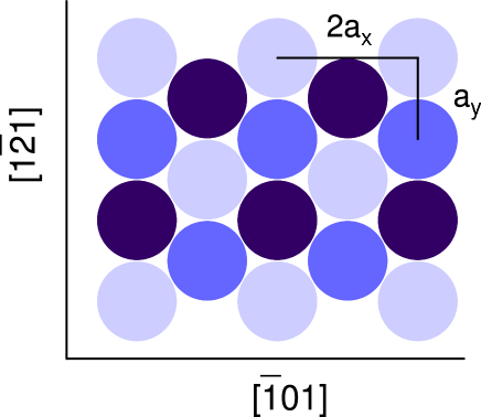
Figure 1: Schematic top view of the bcc(111) surface. Atoms from three successive geometrical layers represent positions of columns in the SOS model. The Z axis is normal to the (111) plane and $a_{x}=a\sqrt{2}/2$, $a_{y}=a\sqrt{6}/3$.

The model is designed for constant coverage of 1 physical monolayer – critical coverage for adsorbate–induced faceting mad99b . This means that each column has exactly one adsorbate atom placed at the highest position. There is also a restriction imposed on column heights: the nearest neighbor column heights can differ only by $\pm 1,\pm 2$.

The surface formation energy can be expressed as interaction energy of columns

$$\begin{array}[]{lll}{\cal H}&=&\frac{1}{2}\sum\limits_{i}\left\{\sum\limits_{j_{1}}{\left[J_{1}\omega_{i,j_{1}}(1)+K_{1}\omega_{i,j_{1}}(2)\right]}\right.\\[12.91663pt] &&+\sum\limits_{j_{2}}{\left[2J_{2}\omega_{i,j_{2}}(0)+\left(2J_{2}+K_{2}\right)\omega_{i,j_{2}}(3)\par\right]}\\ &&+\left.J_{2}\sum\limits_{j_{3}}{\left[\omega_{i,j_{3}}(2)\par+\omega_{i,j_{3}}(4)\par\right]}\right\}+NJ_{0},\end{array}$$ (1)

where the sums over $j_{1}$, $j_{2}$, and $j_{3}$ represent the sums over first, second, and third neighbours of the column at site $i$, respectively. The function $\omega_{i,j}(k)=\delta\left(\left|h_{i}-h_{j}\right|-k\right)$, for $k=0,1,2,\ldots$, is expressed by the Kronecker delta: $\delta(x)=1$ for $x=0$ and $\delta(x)=0$ for $x\neq 0$. Model parameters $J_{0}$, $J_{1}$, $J_{2}$, $K_{1}$, and $K_{2}$ depend on interaction energies between substrate and adsorbate atoms (for details see oleksy ).

It turns out that the energy of the nearest neighbours interaction in the Hamiltonian is conserved. This property follows from symmetry of the model and the restriction imposed on the on column heights. Thus the energy of the nearest neighbours interactions can be treated as the reference energy. Choosing coupling constant $J_{2}$ as the unit of energy, we will work with one model parameter $K=K_{2}/J_{2}$. The dimensionless Hamiltonian $\tilde{\cal H}={\cal H}/J_{2}$, takes the following form

$$\begin{array}[]{lll}\tilde{\cal H}&=&\frac{1}{2}\sum\limits_{i}\left\{\sum\limits_{j_{2}}{\left[2\omega_{i,j_{2}}(0)+\left(2+K\right)\omega_{i,j_{2}}(3)\par\right]}\right.\\[12.91663pt] &&+\left.\sum\limits_{j_{3}}{\left[\omega_{i,j_{3}}(2)+\omega_{i,j_{3}}(4)\right]}\right\}+\tilde{\cal H}_{\mathrm{ref}},\end{array}$$ (2)

In what follows we will use dimensionless energy omitting the tilde and $\tilde{\cal H}_{\mathrm{ref}}$. It has been shown oleksy that the energy of the (211) face is minimal when $-2<K<0$, whereas the (111) surface is stable for $K>0$. For $K<-2$ the (011) face has minimal energy.

III Density of states

In this paper we calculate density of state for the SOS model using a modification of the Wang–Landau method wl_1 proposed by Belardinelli and Pereyrapereyra_1 ; pereyra_2 .

III.1 The Wang – Landau method

The WL method is based on a random walk which produces a flat histogram in the energy space. A trial configuration of energy $E^{\prime}$ is accepted with probability

$$W(E\rightarrow E^{\prime})=min[1,g(E)/g(E^{\prime})],$$ (3)

where E is energy of the current configuration and $g(E)$ means the density of states. However, the $g(E)$ is not known and calculation of the density of states is the main goal of WL method. To achieve this goal, the $g(E)$ is changed after each step of the random walk $g(E)\rightarrow fg(E)$ by a modification factor $f>1$. Moreover, it is assumed that initially $g(E)=1$ for all energies and $f=e$.

Very recently, Belardinelli and Pereyra have demonstrated pereyra_1 saturation of errors in the WL method, or nonconvergence of calculated density of states to the exact value. Moreover, they have shown that if the refinement parameter $\ln f(t)$ depends on time as $\propto t^{-1}$ for large time, the calculated density of states approaches asymptotically to the exact values as $\propto t^{-1/2}$. This fact is used in Belardinelli – Pereyra (BP) modification of the WL method.

To present the BP method let us introduce some quantities. It is assumed that the random walk is performed in the energy range $E_{min}\leq E\leq E_{max}$ with $\Omega$ different energy levels. A Monte Carlo time $t=j/\Omega$ is defined as the number of trial configurations j used so far with respect to the number of energy states $\Omega$. From numerical reason it is convenient to use $S(E)={\ln g(E)}$ and $F=\ln f$ instead of $g(E)$ and $f$. There are two stages in calculation of $S(E)$ in the BP method. In the first stage, the refinement parameter $F$ is changed similarly as in the original WL method, i.e., $F\rightarrow F/2$ when all energy states are visited in the random walk with given F. Please notice that the criterion for flatness of the histogram is not used here. The second stage begins at critical time $t_{c}$ defined as a moment when the new value of $F$ becomes smaller than $1/t$. From this time, the refinement parameter takes the continuous form $F(t)=t^{-1}$. The second stage lasts until the refinement parameter reaches a predefined value $F_{\mathrm{{min}}}$ (typically $F_{\mathrm{{min}}}=10^{-8}$). To control the convergence of S(E,t) during the random walk it is useful to measure the following quantities: the histogram $H(E,t)$ and its averaged value at time t, $\langle H(t)\rangle=\frac{1}{\Omega}\sum_{E}{H(E,t)}$, and the width of the histogram ${\Delta H(t)=H_{\mathrm{{max}}}(t)-H_{\mathrm{{min}}}(t)}$, and the relative width $\delta H(t)=\frac{\Delta H(t)}{\langle H(t)\rangle}$. According to result of Ref.pereyra_2 the quantity $\delta H(t)$ has the same longtime behaviour as the error of $S(E,t)$

$$\delta H(t)\propto t^{-\frac{1}{2}}$$ (4)

As the exact value of $S(E)$ is not known, the time dependence of $\delta H(t)$ can be used to evaluate convergence and the accuracy of BP algorithm.

III.2 Calculation of S(E) for the SOS model

We consider the SOS model on the rectangular lattice with $N_{x}$ and $N_{y}$ columns along x and y axis, respectively, and with periodic boundary conditions. A relation $N_{x}=\frac{7}{6}N_{y}$ is assumed to assure approximate equality of linear lattice sizes along the x and y axis. The linear system size is defined as $L=\sqrt{N_{x}N_{y}}$. The quantity $S(E)=\ln g(E)$ is calculated by performing the the random walk in the energy space with the transition probability given by Eq. (3). At each step a trial configuration is generated by choosing two lattice sites i and j and changing heights of columns at these sites: $(h_{i},h_{j})\rightarrow(h_{i}-3,h_{j}+3)$. Due to constrains imposed on columns height in the SOS model, the change $(h_{i},h_{j})\rightarrow(h_{i}-3,h_{j}+3)$ is allowed only when $h_{i}$ is a local maximum and $h_{j}$ is a local minimum. Local maximum (minimum) at site $k$ denotes that column $h_{k}$ is higher (lower) than its 6 nearest neighbor columns, respectively. In order to speed up calculation we use lists of local maxima and minima and a trial configuration is generated by random choice of a maximum and a minimum.

During the preliminary application of the BP method to the SOS model we encountered a problem of very large $t_{c}$ even for the small linear sizes of the system. Contrary to simulation of Ising model, the number of steps needed to visit each energy level at least once becomes very large even for the first value of the refinement parameter $F_{0}=1$. To overcome this problem, we modify the first stage of the BP method by introducing a separation $s$ between successive increments of S(E) and H(E) in the random walk, similarly as in Ref.bhatt .

The errors $\delta S(E)$ of $S(E)$ are estimated from sample of $m$ independent $S_{1}(E),\ldots S_{m}(E)$ results of simulations and then an average error $\delta S=\frac{\sum_{E}{\delta S(E)}}{\Omega-1}$ is calculated. Having calculated $S(E)$ one can easily investigate temperature dependence of various quantities discussed in the paper:

the energy distribution

$$P(E,T)=\frac{\exp(S(E)-E/T)}{\sum\limits_{E}\exp(S(E)-E/T)},$$ (5)

moments of energy

$$\langle E^{n}\rangle=\frac{\sum\limits_{E}E^{n}\exp(S(E)-E/T)}{\sum\limits_{E}\exp(S(E)-E/T)},$$ (6)

the specific heat per site

$$C=\frac{\langle E^{2}\rangle-\langle E\rangle^{2}}{L^{2}T^{2}},$$ (7)

the Binder’s fourth cumulant

$$V_{4}=1-\frac{\langle E^{4}\rangle}{3\langle E^{2}\rangle^{2}}.$$ (8)

IV Phase Diagram

WL and BP methods can be easily applied to construct a phase diagram for a finite system with competitive interactions by performing the random walk in multi–dimensional energy space. In this paper we construct the phase diagram in ($T$,$K$) plane by use of a modified BP method and performing the random walk in two–dimensional energy space ($E_{J},E_{K}$). To do this the energy of the system, $E=\tilde{\cal H}-\tilde{\cal H}_{\mathrm{ref}}$ from Eq. (2), is decomposed into two parts $E=E_{J}+KE_{K}$, where $KE_{K}$ represents interaction energy with the coupling constant $K$ and $E_{J}$ stands for remaining contribution to $E$.

Having calculated density of states $g(E_{J},E_{K})$ or $S(E_{J},E_{K})=\ln g(E_{J},E_{K})$ one can easily obtain the mean energy $\langle E\rangle$, the specific heat $C$, and other quantities for any value of the coupling constant $K$. For example, the mean energy can be calculated as

$$\langle E(K)\rangle=\frac{\sum\limits_{E_{J}}\sum\limits_{E_{K}}(E_{J}+KE_{K})e^{S(E_{J},E_{K})-\frac{E_{J}+KE_{K}}{T}}}{\sum\limits_{E_{J}}\sum\limits_{E_{K}}e^{S(E_{J},E_{K})-\frac{E_{J}+KE_{K}}{T}}}$$ (9)

This approach is limited to rather small systems because the number of states $\Omega(E_{J},E_{K})$ is much more greater than $\Omega(E)$ in one–dimensional energy space. For example, $\Omega(E_{J},E_{K})$ reaches 82073 and 464162 for $L=26$ and $39$, respectively whereas $\Omega(E)$ amounts to 304 and 718 for $K=-1$. Therefore, we limit study of the phase diagram to two system sizes, $L=26$ and $39$.

In simulations of $S(E_{J},E_{K})$ we used separation $s=4L$ and the refinement parameter $F$ was limited by $F_{\mathrm{{min}}}=10^{-7}$. For such parameters and system size $L=39$ the computation takes about 15 days on a 2.6 GHz Opteron processor.

Figure 2: Phase diagram for system size $L=39$. Labels D, F112, F011, and M denotes disordered, faceted {112}, faceted {011}, and mixed phases, respectively.

On the other hand, the average error of $S(E_{J},E_{K})$ estimated on results of four independent runs, was rather small: $3*10^{-3}$ and $2*10^{-3}$ for $L=26$ and $L=39$, respectively. Hence, this validates the use of $S(E_{J},E_{K})$ to calculate thermodynamical quantities.

To construct the phase diagram in the ($T,K$) plane for a finite system of a linear size $L$ we treat temperature $T_{c}(L,K)$ at which the specific heat has a maximum, as temperature of a phase transition. A simple optimization method – golden section search numrec was applied to locate the maximum of the specific heat as a function of temperature for a given $K$. We also examined temperature dependence of the Binder’s fourth cumulant Eq. (8) because $V_{4}$ has a minimum at a first–order phase transition.

The phase diagram (see Fig. 2) constructed for the lattice size $L=39$ comprises three phases: faceted 112, faceted 011, and disordered. There is also a region between two faceted phases where the mixture of these phases appears. The line separated a faceted phase and the mixed one is determined from location of the additional maximum in the specific heat (see for example Fig. 3). Thus, in this case the first peak corresponds to transition from faceted $112$ phase to the mix one, whereas the second peak is generated by transition from faceted $112$ phase to the disordered phase.

Figure 3: Specific heat with two peaks for $K=-1.90$.

The phase diagram for a smaller linear size $L=26$ has the same qualitative form as the diagram in Fig. 2 but the phase transition lines are slightly shifted due to the finite–size effects. The largest differences are observed for transition temperature from the $F112$ phase to the disordered one (see Fig. 4). In what follows we limit our consideration to this transition because it is observed experimentally song95 ; song07 . Big differences between transition temperatures for these small systems require the finite–size analysis for larger linear system sizes. This can be performed by calculation of density of states in one–dimensional energy space. Inspection of energy distribution indicates that transition between the $F112$ and the disordered phase is of first order phase transition because the energy distribution at transition temperature has the double peak form (see Fig. 5). The first peak represents the $F112$ phase and the second peak represents the disordered phase. The nature of this phase transition is also confirmed by temperature dependence of the Binder’s fourth cumulant $V_{4}$, which has minimum at temperature close to $T_{c}(L)$. Thus, it is enough to perform a detailed analysis for one value of the coupling constant $K$, and we choose the case $K=-1$ to minimize the number of energy states or computing time.

Figure 4: Finite–size effect. The transition line between the faceted F112 and disordered D phases. Continuous (dashed) line represent system size $L$ 39 (26), respectively.

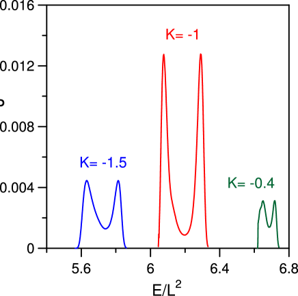
Figure 5: Energy distribution at transition temperature for three values of $K$ and system size $L=39$.

V Finite–size scaling

The $S(E)$ is calculated for the coupling constant $K=-1$ in a single energy interval $(E_{\mathrm{min}},E_{\mathrm{max}})$ in order to avoid boundaries errors caused by partition of energy space into several pieces. It is especially important in a case of first order phase transition, where at transition temperature $T_{c}$, the energy distribution Eq. ( 5) has two peaks of equal heights at $E=E_{-}$ and $E=E_{+}$. In our case the interval $(E_{-},E_{+})$ makes up about $1/3$ of the whole energy interval. The energy of planar face (111) is chosen as $E_{\mathrm{max}}$ and this state has known degeneracy $g(E_{\mathrm{max}})=1$. On the other hand, it is difficult to reach states close to the minimal energy due to edge energies, hence we choose $E_{\mathrm{min}}$ as small as possible to assure convergence of $S(E)$.

To study the size dependence of some physical quantities the following numbers $L$ where used in calculations 26, 39, 52, 65, 78, 91, and 104. For each value of $L$ the $S(E)$ was calculated until refinement parameter $F$ reached the minimal value $F_{\mathrm{{min}}}=10^{-8}$. Values of separation $s$ used in the first stage of BP method were comparable with the number of energy states ($s\approx 0.7\Omega$). To estimate errors of $S(E)$ each calculation were repeated 5 times and average density was obtained. The relative averaged error of $S(E)$ was smaller than $3\times 10^{-4}$ for $L<104$ and $1.4\times 10^{-3}$ for $L=104$. The increase of the error of $S(E)$ for the largest size studied here was caused by large fluctuation of the histogram in the low energy range. Therefore, we did not study the systems with sizes $L>104$.

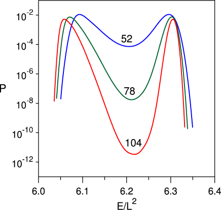
Figure 6: A semi–log plot of energy distribution at transition temperature for 3 linear sizes of system.

V.1 Scaling of transition temperature

We calculated $T_{c}$ using fact, that the energy distribution Eq. ( 5) has two peaks of equal heights at $T=T_{c}$. The results presented in Fig. 6 demonstrate that $P(E,T_{c})$ has two maxima: the first at energy $E_{-}$ of faceted phase and the second at energy $E_{+}$ of disordered phase. The minimum between these peaks becomes deeper as system sizes increases. The probability to find the system at minimum $P(E_{\mathrm{min}})$ is $7\times 10^{-3}$, $2\times 10^{-6}$ and $3\times 10^{-10}$ of $P(E_{\pm})$ for system size $L$ 52, 78, and 104 respectively. From energy distributions at $T=T_{c}(L)$ one can calculate the free–energy barrier $\Delta{\cal F}(L)=-T_{c}(\ln P(E_{\mathrm{min}},L)-\ln P(E_{-},L))$ which should scale as $\Delta{\cal F}(L)\sim L^{d-1}$ at a first order transition kosterlitz91 . This scaling is confirmed in our calculation because for $L>50$ the free–energy barrier has a linear form fitted by $\Delta{\cal F}(L)=0.354L-13.01$.

Having calculated $T_{c}(L)$ for several linear system sizes we study scaling of $T_{c}(L)$ to calculate the transition temperature in the limit $L\rightarrow\infty$. Our results agree with theory of scaling at first order phase transition

$$T_{c}(L)=T_{c}+a_{1}L^{-2}+a_{2}L^{-4}$$ (10)

The second term proportional to $L^{-4}$ is needed for system size $L<75$ (see Fig. 7). The transition temperature $T_{c}=1.12852$ is obtained from fitting the results with $L>50$ by the function from Eq. (10). Similar result $T_{c}=1.12829$ is obtained by applying the Burlisch –Stoer extrapolation numrec to $T_{c}(L)$. We also studied scaling of temperature $T^{s}_{c}(L)$ at which the specific heat has a maximum in system of linear size $L$. The differences between $T_{c}(L)$ and $T^{s}_{c}(L)$ are of order $10^{-4}$ and extrapolation of $T^{s}_{c}(L)$ for $L\rightarrow\infty$ yields $T_{c}=1.12837$. From these two results we estimate transition temperature for $K=-1$ as $T_{c}=1.12844\pm 0.00008$.

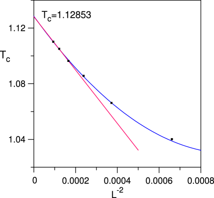
Figure 7: Transition temperature versus $L^{-2}$. Errors are smaller than the symbol size. Thin and thick lines denote linear (in $L^{-2}$) and non-linear fitting of simulation result by the scaling function (Eq. (10)).

V.2 Scaling of specific heat

We found that scaling of the specific heat of the system discussed in this paper can be well described by the function of the form used by Challa et al. challa86 for q–state Potts model.

$$C(L)=\frac{L^{2}Q^{2}(L)D}{{\left[\exp(X(L))+D\exp(X(L))\right]}^{2}},$$ (11)

where

$$Q(L)=\frac{E_{+}(L)-E_{-}(L)}{L^{2}T_{c}},$$

and

$$X(L)=\frac{L^{2}Q(L)}{2T}\left(T-T_{c}(L)\right).$$

The parameter $D$ in Eq. (11) replaces the expression $q(C_{-}/C_{+})^{1/2}$ for the q–state Potts model. The value of $D=1.62$ minimizes the sum of deviation of simulated data from the scaling function for $L>60$.

As seen in Fig. 8, the scaling function (Eq. (11)) well describes the shape of the specific heat near transition temperature $T_{c}(L)$ for $L>60$. For smaller systems studied here ( $L<60$ ) this scaling does not apply – it yields incorrect position and height of specific heat maximum.

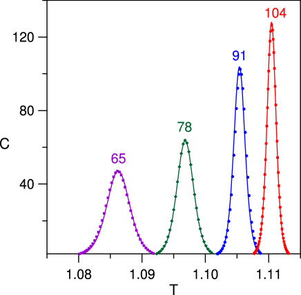
Figure 8: Scaling of the specific heat. Line represents the scaling function (Eq. (11)), symbols represent simulation data and label denotes linear system size $L$.

VI Disordered phase

A nature of disordered phase is not clear. LEED experiment results song95 suggested existence of flat phase above the faceting temperature. On the other hand, previous MC simulationoleksy indicated that this phase is not flat one but disordered faceted phase characterized by chaotic hill–and–valley structure which comprises of randomly distributed small facets mainly of {112} orientation. To clarify this problem we study the size–dependence of the mean–square width of the surface

$${\delta h}^{2}=\left<\frac{1}{L^{2}}\sum\limits_{j}{\left(h_{j}-\bar{h}\right)^{2}}\right>,$$ (12)

where sum runs over lattice sites and $\bar{h}$ is the arithmetic average of column heights. This quantity has been used in investigation of roughening transition tosat96 ; jaszczak97 ; jaszczak97ss in SOS models because ${\delta h}^{2}$ as function of a system size $L$ has logarithmic dependence in the rough phase.

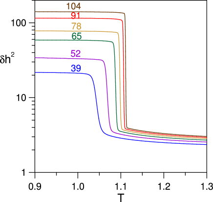
Figure 9: Semi–log plot of ${\delta h}^{2}$ versus $T$ for several lattice sizes $L$.

In order to investigate the dependence of ${\delta h}^{2}$ on temperature and system size $L$ we computed the microcanonical averages ${\delta h}^{2}(E)$ for each energy state in systems with $L<105$. The microcanonical averages ${\delta h}^{2}(E)$ were calculated by performing the random walk in the energy space using earlier computed densities of states $g(E)$ via BP method. To assure high accuracy of ${\delta h}^{2}(E)$ each state $E$ was visited on average $10^{9}$ times.

The canonical average ${\delta h}^{2}(T)$ is obtained as

$${\delta h}^{2}(T)=\frac{\sum\limits_{E}{\delta h}^{2}(E)\exp(S(E)-E/T)}{\sum\limits_{E}\exp(S(E)-E/T)}$$ (13)

This way of calculating ${\delta h}^{2}(T)$ is similar to a method of computing moments of magnetization schulz05 .

Simulation results show (see Fig. 9) that ${\delta h}^{2}(T)$ is decreasing function of temperature and it rapidly changes at transition temperature $T_{c}(L)$. On the other hand, ${\delta h}^{2}$ is increasing function of linear system size $L$. In the high–temperature phase ${\delta h}^{2}$ scales logarithmically with $L$ in the whole temperature range $T>T_{c}$ (see Fig. 10) and results of simulations are very well fitted by the function

$${\delta h}^{2}(T,L)=A(T)\ln L+B(T)$$ (14)

The amplitude $A$ has the largest value at $T=T_{c}$ and it decreases down to a saturation value 0.4625 for $T>T_{c}$ (see Fig. 11).

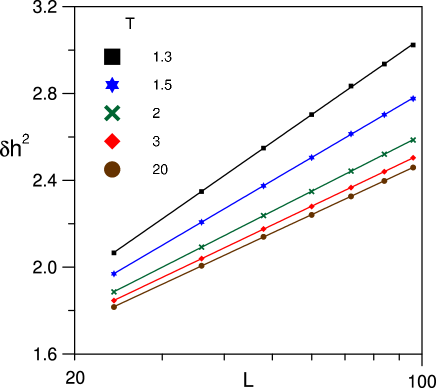
Figure 10: Semi–log plot of size–dependence of ${\delta h}^{2}$ at several temperatures $T$.

Figure 11: Plot of amplitude $A$ versus temperature $T$.

The logarithmic dependence of the mean–square width of the surface on linear size of the system indicates that the disordered phase is a rough phase. Hence, the faceting transition is the first–order roughening phase transition. On the other hand, the surface above $T_{c}$, has a disordered hill–and–valley structure as follows from Monte Carlo simulations (see e.g. Fig. 5 in Ref.oleksy ). Hence, this is different type of rough surface than that observed in typical roughening transition where a surface becomes rough by formation of stepsjaszczak97ss .

VII Discussion

It is demonstrated that the Wang–Landau method can be applied to construct a phase diagram for a system with competitive interactions if one performs calculations of density of states in a special two–dimensional energy space. From such density of states one can compute thermodynamical quantities for any value of interaction energies. Then one can find phase transition lines and nature of transitions. However such approach is limited to rather small linear sizes ( in our case for $L<40$) due to huge numbers of states occurring in two–dimensional energy space. Because of that, a finite–size analysis should be performed for chosen values of interaction energies to find the order of the phase transition, transition temperature and other interesting quantities.

We found that transition from faceted {112} phase to high–temperature phase is of first order because the energy distribution has double–peak form at transition temperature. The transition temperature scales as $L^{-2}$ for large linear system size $L$, but higher order corrections are needed to the scaling for $L<75$. Scaling of the specific heat is well described by the function of the form used by Challa et al. challa86 for q–state Potts model.

In order to clarify the nature of high–temperature phase we calculated the mean–square width of the surface ${\delta h}^{2}$. Experimental resultssong95 suggest that surface becomes flat above transition temperature. However, investigation of surface morphology in high temperatures is not so easy. In most of experiments, such investigations are performed after quick cooling the sample to low temperatures. In case of adsorbate induced faceting, attempts of freezing of high–temperature phase were always failed for available cooling ratessong95 . On the other hand, the nature of high–temperature phase can be easy investigated in the SOS model via the Wang–Landau method. We found that the mean–square width of the surface depends logarithmically on the linear system size above the transition temperature. This means that surface is rough above the faceting transition temperature. However, this rough surface has disordered hill–and–valley structure and differs from typical rough phase observed in roughening transitionjaszczak97ss .

References

- (1) K.-J. Song, J. C. Lin, M. Y. Lai, and Y. L. Wang, Surf. Sci. 327, 17 (1995).
- (2) T. E. Madey, J. Guan, C.-H. Nien, C.-Z. Dong, H.-S. Tao, and R. A. Campbell, Surf. Rev. Lett. 3, 1315 (1996).
- (3) T. E. Madey, C.-H. Nien, K. Pelhos, J. J. Kolodziej, I. M. Abdelrehim, and H.-S. Tao, Surf. Sci. 438, 191 (1999).
- (4) C.-H. Nien, T. E. Madey, Y. W. Tai, T. C. Leung, J. G. Che, and C. T. Chan, Phys. Rev. B 59, 10335 (1999).
- (5) Y.-W. Liao, L. H. Chen, K. C. Kao, C.-H. Nien, M.-T. Lin, and K.-J. Song, Phys. Rev. B 75, 125428 (2007).
- (6) J. G. Che, C. T. Chan, C. H. Kuo, and T. C. Leung, Phys. Rev. Lett. 79, 4230 (1997).
- (7) T. E. Madey, W. Chen, H. Wang, P. Kaghazchi, and T. Jacob, Chem. Soc. Rev. 37, 2310 (2008).
- (8) T.-Y. Fu, L.-C. Cheng, C.-H. Nien, and T.T. Tsong, Phys. Rev. B 64, 113401 (2001).
- (9) A. Szczepkowicz and R. Bryl, Phys. Rev. B 71, 113416 (2005).
- (10) A. Szczepkowicz, A. Ciszewski, R. Bryl, C. Oleksy, C.-H. Nien, Q. Wu, and T. E. Madey, Surf. Sci. 559, 55 (2005).
- (11) H.-S. Kuo, I.-S. Hwang,T.-Y. Fu, Y.-H. Lu, C.-Y. Lin, and T.T. Tsong, Appl. Phys. Lett. 92, 063106 (2008).
- (12) C.-C. Chang, H.-S. Kuo, I.-S. Hwang and T.T. Tsong, Nanotechnology 20, 115401 (2009).
- (13) G. Mazzeo, E. Carlon, and H. van Beijeren, Phys. Rev. Lett. 74, 1391 (1995).
- (14) G. Santoro, M. Vendruscolo, S. Prestipino, and E. Tosatti, Phys. Rev. B 53, 13169 (1996).
- (15) D. L. Woodraska and J. A. Jaszczak, Phys. Rev. Lett. 78, 258 (1997).
- (16) D. L. Woodraska, J. A. Jaszczak, Surf. Sci. 374, 319 (1997).
- (17) V. P. Zhdanov and B. Kaseno, Phys. Rev. B 56, R10067 (1997).
- (18) C. Oleksy, Surf. Sci. 549, 246 (2004).
- (19) D. Niewieczerzal and C. Oleksy, Surf. Sci. 600, 56 (2006).
- (20) J. Lee and J. M. Kosterlitz, Phys. Rev. B 43, 3265 (1991).
- (21) F. Wang and D. P. Landau, Phys. Rev. Lett. 86, 2050 (2001).
- (22) F. Wang and D. P. Landau, Phys. Rev. E 64, 056101 (2001).
- (23) S.-H. Tsai, F. Wang, and D. P. Landau, Phys. Rev. E 75, 061108 (2007).
- (24) S. Piccinin and C. Stampfl, Phys. Rev. B 81, 155427 (2010).
- (25) R. E. Belardinelli and V. D. Pereyra, J. Chem. Phys. 127, 184105 (2007).
- (26) R. E. Belardinelli and V. D. Pereyra, Phys. Rev. E 75, 046701-1 (2007).
- (27) C. Zhou and R. N. Bhatt, Phys. Rev. E 72, 025701(R) (2005).
- (28) W. H. Press, B. P. Flannery, S. A. Teukolsky, and W. T. Vetterling, Numerical Recipies. The Art of Scientific Computing, Cambridge University Press, (Cambridge, 1986).
- (29) M. S. S. Challa, D. P. Landau, and K. Binder, Phys. Rev. B 34, 1841 (1986).
- (30) B. J. Schulz and K. Binder, Phys. Rev. E 71, 046705 (2005).