A quantum Monte Carlo study of the ground state chromium dimer

Abstract

We report variational and diffusion quantum Monte Carlo (VMC and DMC) studies of the binding curve of the ground-state chromium dimer. We employed various single determinant (SD) or multi-determinant (MD) wavefunctions multiplied by a Jastrow fuctor as a trial/guiding wavefunction. The molecular orbitals (MOs) in the SD were calculated using restricted or unrestricted Hartree-Fock or density functional theory (DFT) calculations where five commonly-used local (SVWN5), semi-local (PW91PW91 and BLYP), and hybrid (B1LYP and B3LYP) functionals were examined. The MD expansions were obtained from the complete-active space SCF, generalized valence bond, and unrestricted configuration interaction methods. We also adopted the UB3LYP-MOs to construct the MD expansion (UB3LYP-MD) and optimized their coefficients at the VMC level. In addition to the wavefunction dependence, we investigated the time-step bias in the DMC calculation and the effects of pseudopotentials and backflow transformation for the UB3LYP-SD case. Some of the VMC binding curves show a flat or quite shallow well bottom, which gets recovered deeper by DMC. All the DMC binding curves have a minimum indicating a bound state, but the comparison of atomic and molecular energies gives rise to a negative binding energy for all the DMC as well as VMC calculations.

I Introduction

The chromium dimer (Cr₂) has attracted a lot of attention as a prototype to understand the $d$-$d$ binding in both experimental Michalopoulos_etal_1982 ; Bondybey_English_1983 ; Simard_etal_1998 ; Hilpert_Ruthardt_1987 ; Su_etal_1993 ; Casey_Leopold_1993 ; Moskovits_etal_1985 and theoretical studies McLean_Liu_1983 ; Richman_McCullough_1987 ; Walch_etal_1983 ; Wood_etal_1980 ; Goodgame_Goddard_1981 ; Goodgame_Goddard_1985 ; Anderson_etal_1994 ; Anderson_Roos_1995 ; Anderson_etal_1996 ; Celani_etal_2004 ; Mitrushenkov_Palmieri_1997 ; Angeli_etal_2002 ; Angeli_etal_2006 ; Scuseria_1991 ; Baushlicher_Partridge_1994 ; Meuller_etal_2009 ; Stoll_Werner_1996 ; Atha_Hillier_1982 ; Kok_Hall_1983 ; Vissher_etal_1994 ; Dachsel_etal_1999 ; Takahara_eta_1989 ; Moritz_etal_2005 ; Kurashige_Yanai_2009 ; Delley_etal_1983 ; Bernholc_Hozwarth_1983 ; Dunlap_1983 ; Baykara_etal_1984 ; Painter_1986 ; Edgecombe_Becke_1995 ; Cheng_Wang_1996 ; Desmarais_etal_2000 ; Yanagisawa_etal_2000 ; Barden_etal_2000 ; Valiev_etal_2003 ; Furche_Perdew_2006 ; Calaminici_etal_2007 ; Gutsev_Bauschlicher_2003 ; Thomas_etal_1999 ; Kitagawa_etal_2007 ; Shi-Ying_2008 ; Tsuchimochi_etal_2010 . The ground state is experimentally observed to be a singlet state, ${}^{1}\Sigma_{g}^{+}$Michalopoulos_etal_1982 , whereas the ground state of the constituent Cr atom $3d^{5}4s^{1}$ (${}^{7}S$) has the highest spin multiplicity in the $3d$ atoms. Recent spectroscopic experiments reported an equilibrium bond length ($R_{e}$) and binding energy ($D_{e}$) of 1.6788 ÅBondybey_English_1983 and 1.53 $\pm$ 0.05 eVSimard_etal_1998 , respectively (some older experiments reported $R_{e}$ of 1.68 ÅMichalopoulos_etal_1982 and $D_{e}$ of 1.44 $\pm$ 0.05 eV Hilpert_Ruthardt_1987 and 1.42 $\pm$ 0.10 eV Su_etal_1993 ). However, no theoretical study has provided a quantitatively satisfactory result for Cr₂ so far, since its chemical binding is rather complicated.

From the theoretical viewpoint, there are two extremely different pictures to understand the chemical binding in Cr₂ qualitatively. The first one is based on elementary molecular orbital (MO) theories. In this framework, Cr₂ is treated as a closed shell (single-determinant) state, with all the bonding orbitals occupied ($1\sigma_{g}^{2}2\sigma_{g}^{2}1\pi_{u}^{4}1\delta_{g}^{4}$, arising from the $3d$ and $4s$ orbitals). Cr₂ is therefore interpreted as having a sextuple bond, which is the highest multiple bond in any diatomic molecule. This is naively consistent with the observed short bond length ($\approx$ 1.68 Å) Michalopoulos_etal_1982 ; Bondybey_English_1983 , whereas the experimental $D_{e}$ ($\approx$ 1.5 eV) is rather small in the context of multiple bonds, which is smaller than that of singly bonded Cu₂ ($\approx$ 2.0 eV). This fact may imply that an elementary one-electron approximation picture is invalid for Cr₂ and hence “non-dynamical” (static) correlation effects are important. Indeed, restricted Hartree-Fock (RHF) does not only give an incorrect dissociation behavior, but also gives rise to a ground state energy of Cr₂ far above that of the two isolated atoms (about 20 eV higher)Goodgame_Goddard_1981 .

The second picture, which is the extreme opposite to the first one, emphasizes the relative stability of high-spin atomic statesGoodgame_Goddard_1981 . This is the molecular analogue of antiferromagnetism and can be treated at the crudest level of theory by the unrestricted (or broken symmetry) Hartree-Fock (UHF) theory using a spin unrestricted single-determinant of symmetry broken molecular spin orbitalsTakahara_eta_1989 ; Kitagawa_etal_2007 . The method can approximately deal with the static correlation effects. Up and down-spin electrons are antiferromagnetically localized on each of the Cr atoms, where the charge density has a $D_{\infty h}$ symmetry but the spin density has a $C_{\infty v}$ symmetry. The wavefunction represents the nearest possible single-determinant approximation to the ${}^{1}\Sigma_{g}^{+}$ state, but it is not an eigenfunction of total spin, leading to spin contamination. This can be easily remedied by a properly symmetrized multi-determinant expansion of the UHF wavefunction, i.e., the generalized valence bond (GVB) method. However, the GVB method gives rise to a very weakly bound molecule ($D_{e}=0.35$ eV) with a very long bond length ($R_{e}=3.1$ Å)Goodgame_Goddard_1981 . Although a complete active space (CAS) self-consistent field (SCF) method can also consider the static correlation, a typical CASSCF with a 12 orbital active space and 12 active electrons, CASSCF(12,12), provides a poor result of $R_{e}$ and $D_{e}$, similar to GVB Kitagawa_etal_2007 . These disagreements with experiments indicate dynamical correlation effects are also important for achieving quantitatively satisfactory results. In summary, the chemical binding in Cr₂ involves a highly complicated blend of $4s$-$4s$ and $3d$-$3d$ interactions with antiferromagnetic coupling.

To understand such a complicated binding mechanism, a large number of ab initio studies have been performed based on either traditional MO theoriesMcLean_Liu_1983 ; Richman_McCullough_1987 ; Walch_etal_1983 ; Wood_etal_1980 ; Goodgame_Goddard_1981 ; Goodgame_Goddard_1985 ; Anderson_etal_1994 ; Anderson_Roos_1995 ; Anderson_etal_1996 ; Celani_etal_2004 ; Mitrushenkov_Palmieri_1997 ; Angeli_etal_2002 ; Angeli_etal_2006 ; Scuseria_1991 ; Baushlicher_Partridge_1994 ; Meuller_etal_2009 ; Stoll_Werner_1996 ; Atha_Hillier_1982 ; Kok_Hall_1983 ; Vissher_etal_1994 ; Dachsel_etal_1999 ; Takahara_eta_1989 ; Moritz_etal_2005 ; Kurashige_Yanai_2009 or density functional theories (DFT) Delley_etal_1983 ; Bernholc_Hozwarth_1983 ; Dunlap_1983 ; Baykara_etal_1984 ; Painter_1986 ; Edgecombe_Becke_1995 ; Cheng_Wang_1996 ; Desmarais_etal_2000 ; Yanagisawa_etal_2000 ; Barden_etal_2000 ; Valiev_etal_2003 ; Furche_Perdew_2006 ; Calaminici_etal_2007 ; Gutsev_Bauschlicher_2003 ; Thomas_etal_1999 ; Kitagawa_etal_2007 ; Shi-Ying_2008 ; Tsuchimochi_etal_2010 . In MO, both single- and multi-reference theories were studied. Within the single-reference theory, the coupled-cluster approach with single and double excitations including triples noniteratively, CCSD(T), is one of the most accurate methods. Restricted CCSD(T) calculations give a very weak binding ($D_{e}=0.38$ eV) with a short bond length ($R_{e}=1.60$ Å), whereas unrestricted CCSD(T) calculations provide a better binding energy ($D_{e}=0.89$ eV), but with a longer bond length ($R_{e}=2.54$ Å). In multi-reference theories, a typical reference is a CASSCF(12,12) calculation which is responsible for the static correlation. Using the CAS reference, dynamical correlation can be taken into account by multi-reference configuration interaction (MRCI)Dachsel_etal_1999 , coupled cluster (MRCC)Meuller_etal_2009 , or second-order perturbation (CASPT2) methodsAnderson_etal_1994 . Although these multi-reference methods give a better $R_{e}$ than single-reference methods, there is still room to improve further the accuracy of $D_{e}$.

In DFT, various exchange-correlation (XC) functionals are available such as the local (spin) density approximation (LDA/LSDA), the generalized gradient approximation (GGA), as well as the hybrid XC functionals. Both restricted LDA (RLDA) and the unrestricted formalism (ULDA) give rise to overbinding, i.e., too short $R_{e}$ and too large $D_{e}$ Delley_etal_1983 ; Bernholc_Hozwarth_1983 ; Dunlap_1983 ; Baykara_etal_1984 ; Painter_1986 , which is a well-known failure of LDA. Both restricted and unrestricted GGA calculationsEdgecombe_Becke_1995 ; Thomas_etal_1999 ; Desmarais_etal_2000 ; Yanagisawa_etal_2000 ; Barden_etal_2000 ; Valiev_etal_2003 ; Gutsev_Bauschlicher_2003 ; Furche_Perdew_2006 ; Calaminici_etal_2007 generally improve the LDA discrepancy, but it is difficult to choose the “best” GGA functional because one may give a better $R_{e}$, but it may give a worse $D_{e}$, and vice versa. Restricted B3LYP, though it is popular for covalent molecules, gives rise to an unbound molecular stateEdgecombe_Becke_1995 ; Kitagawa_etal_2007 . Although unrestricted B3LYP reproduces a bound state, it provides a smaller $D_{e}$ of $\approx 1.0$ eV with much larger $R_{e}$ of $\approx 2.5$ ÅEdgecombe_Becke_1995 ; Kitagawa_etal_2007 . These results may imply that the difficulties for the binding of Cr₂ would originate from a delicate balance between exchange and correlation in DFT for chemical binding of Cr₂.

Quantum Monte Carlo (QMC) methodsHammond_Lester_Reynolds_1994 ; Foulkes_Mitas_Needs_Rajagopal_2001 are one of the most accurate techniques in state-of-the-art ab-initio calculations for quantitative descriptions of electronic structures. There are two typical QMC calculations, i.e., variational and diffusion Monte Carlo (VMC and DMC) methods. VMC is not usually accurate enough since its result strongly depends on the correlated trial wavefunction adopted. DMC is a technique for numerically solving the many- electron Schödinger equation for stationary states using imaginary time evolution. The fixed-node approximation is usually assumed to maintain the fermionic anti-symmetry in DMC. Although the fixed-node DMC can accurately evaluate the ground state energy of many atoms and molecules using only the trial node from a single determinant (SD), it sometimes fails, especially for “near-degeneracy” systems such as the Be atom. This implies that the fixed-node DMC method can work well for the dynamic correlation, but not for the static correlation which should be included at the stage of choosing the fixed-node trial wavefunction. The Cr₂ molecule is also considered as a near-degeneracy molecular system and hence a good challenge to QMC.

In this study we performed VMC and DMC calculations of Cr₂ with several choice of trial wavefunctions. Variety of the XC functionals are examined to construct orbital functions including HF, SVWN LDA, PW91 and BLYP GGA, B1LYP and B3LYP hybrid functionals, with both restricted and unrestricted treatments. In addition to a single-determinant form of the many-body wavefunction, we also tried several multi-determinant (MD) forms. For the orbital part we also introduced the backflow transformation FEY56 ; DRU06 ; RIO06 . Performance of the XC functionals are examined based on the variational principle with respect to the fixed node Hammond_Lester_Reynolds_1994 ; Foulkes_Mitas_Needs_Rajagopal_2001 . The chemical binding of the ground-state Cr₂ may be examined in two ways: (i) use of the binding curve and (ii) a comparison of atomic and molecular energies.

The present paper is organized as follows: Section II describes the present computational methods. Section III provides numerical results and discussion. Section IV summarizes the present study.

II Computational methods

We replaced the inner Neon core (10 core electrons) of the Cr atom with a small core norm-conserving pseudopotential which is constructed from Dirac-Fock atomic solutions. More specifically we employed the Lee-Needs (LN) soft pseudopotential LEE00 using Troullier-Martins construction. To check the dependence on the potential we also used a small core Burkatzki-Filippi-Dolg (BFD) pseudopotential BUR08 . An electronic many-body wavefunction is composed of anti-symmetrized products of orbital functions which is generated from DFT or HF. Various XC functionals give different orbitals from which different structures of the nodal surface CEP91 of the many-body wavefunction (the surface in configuration space on which the wavefunction is zero and across which it changes sign) are constructed. For different nodal structures, we can exploit the variational principle to see which choice is better, comparing the ground state energyWAG03 . In this study we tested several combinations of (i) the choice of XC, (ii) spin restricted/unrestricted treatment of orbitals, (iii) SD/MD, (iv) choice of pseudopotentials, and (v) with/without backflow degrees of freedomFEY56 .

In VMC the ground state energy is evaluated as the expectation value of the Hamiltonian $\hat{H}$ with a many-body trial wavefunction, $\Psi$,

$$E=\frac{\int\Psi^{*}\hat{H}\Psi\,d{\bf R}}{\int\Psi^{*}\Psi\,d{\bf R}}=\frac{\int|\Psi|^{2}\Psi^{-1}\hat{H}\Psi\,d{\bf R}}{\int|\Psi|^{2}\,d{\bf R}},$$ (1)

where $\bf R=\left({\bf r}_{1},...,{\bf r}_{N}\right)$ denotes an electronic configuration of valence electrons in a molecule ($N=28$ with 14 up and down spins, respectively, for Cr₂), and the energy has been written as an average of the local energy, $E_{L}\left({\bf R}\right)=\Psi^{-1}\hat{H}\Psi$, over the probability distribution $p({\bf R})=|\Psi|^{2}/\int|\Psi|^{2}\,d{\bf R}$. The energy expectation value is evaluated from Monte Carlo integration, using the Metropolis algorithm to generate electronic configurations distributed according to $p({\bf R})$.

In the DMC method the ground-state component of a trial wavefunction which overlaps with the exact one is projected out by evolving an ensemble of electronic configurations using the imaginary-time Schrödinger equation. Attempts to carry out this procedure exactly result in a “fermion sign problem”, which is circumvented by constraining the nodal surface of the wavefunction to equal that of the trial wavefunction. The DMC energy calculated with this fixed-node constraint is equal or higher than the exact ground-state energy, and becomes equal to the exact one if and only if the fixed nodal surface is exact.

We used the many-body wavefunction taking the form,

$$\Psi\left({\bf R}\right)=e^{J\left({\bf R}\right)}\cdot F_{\rm AS}\left({{\bf r}_{1},\cdots,{\bf r}_{N}}\right)\ ,$$ (2)

where $F_{\rm AS}\left({{\bf r}_{1},\cdots,{\bf r}_{N}}\right)$ is the anti-symmetrized products of orbital functions $\left\{\psi_{i}^{\sigma}\left({\bf r}_{j}\right)\right\}$ such as a Slater determinant. In this study the function is expanded as

$$F_{\rm AS}\left({{\bf r}_{1},\cdots,{\bf r}_{N}}\right)=\sum\limits_{i=0}^{N_{MD}^{\uparrow}}\sum\limits_{j=0}^{N_{MD}^{\downarrow}}c_{ij}\cdot D_{i}^{\uparrow}\left(\tilde{\bf r}_{1},\cdots,\tilde{\bf r}_{{N\mathord{\left/{\vphantom{N2}}\right.\kern-1.2pt}2}}\right)D_{j}^{\downarrow}\left(\tilde{\bf r}_{{N\mathord{\left/{\vphantom{N2}}\right.\kern-1.2pt}2}+1},\cdots,\tilde{\bf r}_{N}\right)\ ,$$ (3)

by determinants with coefficients $c_{ij}$. $D_{0}^{\sigma=\uparrow,\downarrow}\left(\tilde{\bf r}_{1},\cdots,\tilde{\bf r}_{N/2}\right)$ is the ground-state single Slater determinant formed only by the occupied orbitals for each spin, and $D_{j\neq 0}^{\sigma}=\hat{P}_{n\to m}^{\left(j\right)}\cdot D_{0}^{\sigma}$ corresponds to excited state configurations, where $\hat{P}_{n\to m}^{\left(j\right)}$ denotes the excitation from the occupied state $\psi_{n}^{\sigma}\left({\bf r}_{j}\right)$ into the virtual state $\psi_{m}^{\sigma}\left({\bf r}_{j}\right)$. In Eq. ​(3) arguments with a tilde $\tilde{\bf r}_{i}={\bf r}_{i}+{\bf\xi}_{i}\left({\bf r}_{1},\cdots,{\bf r}_{N}\right)$, denote the backflow shift FEY56 . $N_{\rm MD}^{\sigma}=0$ corresponds to SD, and $c_{ij}=c_{i}\cdot\delta_{ij},D_{i}^{\uparrow}=D_{i}^{\downarrow}$ to a spin restricted wavefunction. The orbital functions, $\left\{\psi_{i}^{\sigma}\left({\bf r}_{j}\right)\right\}$, were expanded with a contracted Gaussian basis set (17s18p15d6f)/$\left[{\rm 8s8p7d3f}\right]$. Gaussian03Gaussian03 was used for SCF calculations, while we used CASINO ver.3.0CASINO for QMC calculations. Some calculations (HF and GVB) were carried out using GAMESSGAM93 for SCF and QWalkQWA09 for QMC. We attempted to use another many-body wavefunction form, Pfaffian BAJ06 , which is available in QWalk. However an optimization procedure for the off-diagonal elements of the Pfaffian did not work well and then we could not obtain reliable results, so not reported here in detail.

As for the Jastrow factor $e^{J\left(\bf R\right)}$JAS55 , the function $J\left(\bf R\right)$ is given as DRU04 ,

$$J\left(\bf R\right)=\sum\limits_{i=1}^{N-1}{\sum\limits_{j=i+1}^{N}{u\left({r_{ij}}\right)}+\sum\limits_{I=1}^{N_{\rm ions}}{\sum\limits_{i=1}^{N}{\chi_{I}\left({r_{iI}}\right)}+\sum\limits_{I=1}^{N_{\rm ions}}{\sum\limits_{i=1}^{N-1}{\sum\limits_{j=i+1}^{N}{f_{I}}}}}}\left({r_{iI},r_{jI},r_{ij}}\right),$$ (4)

where suffices $i,j$ and $I$ specify electronic and ionic positions, respectively. Each term, $u$, $\chi$, and $f$, takes into account the dynamical correlation due to electron-electron, electron-nucleus, and electron-electron-nucleus coalescence, respectively. Cutoff lengths are introduced to make each term quadratically fall off to zero at the radius. Specific forms used in each QMC code are described in the appendix. The electron-electron cusp condition KAT57 is imposed in the $u$-term. Variational parameters in $J\left(\bf R\right)$ are designed to be able to include spin polarized case and are optimized by VMC individually at each bond length with fixed cutoff lengths. Those parameters were optimized by the variance minimization DRU05 as well as the energy minimization UMR05 procedures. The backflow shift FEY56 , ${\bf\xi}_{i}\left({\left\{{{\bf r}_{i}}\right\}}\right)={\bf\xi}_{i}^{ee}\left({\left\{{{\bf r}_{ij}}\right\}}\right)+{\bf\xi}_{i}^{eN}\left({\left\{{{\bf r}_{iI}}\right\}}\right)$, is introduced to modify the nodal surface variationally. Each term, $ee$ and $eN$, is expanded with the power of inter-particle distances (up to 8th order in this study) with proper cutoff radii which are fixed in the same values as those in $u$ and $\chi$ in our Jastrow factor DRU06 ; RIO06 . The parameters in the backflow were optimized by the filtered reweighted variance minimization scheme DRU05 allowing spin polarized degrees of freedom.

For the singlet Cr₂ ground stateMichalopoulos_etal_1982 ; Bondybey_English_1983 ; Simard_etal_1998 ; Hilpert_Ruthardt_1987 ; Su_etal_1993 ; Casey_Leopold_1993 ; Moskovits_etal_1985 the spin restricted SCF treatment seems not to give a proper description of localized spin polarization on atomic sites SZA89 . Even using the restricted nodal surface, however, the DMC projection can still recover the proper localized spin polarization. Indeed we found the RHF nodal surface gives a variationally better description than the UHF one. We therefore investigated spin restricted methods as a possibility as well as unrestricted ones. In order to generate the nodal surface, we employed five commonly-used XC functionals, SVWN5(LDA), PW91PW91 and BLYP (GGA), B1LYP and B3LYP(hybrid), shown in Table. 1.

For DMC we started statistical accumulations of 2,000 walkers after equilibration of 1,000 steps with $\delta t$= 0.01[a.u.], for which we have confirmed that the time step bias is within the statistical noise considered here. The present non-local pseudopotentials were evaluated by the T-move scheme CAS06 which is devised to reduce the instability and bias due to the locality approximation MIT91 .

III Results and Discussion

III.1 Single determinant calculations

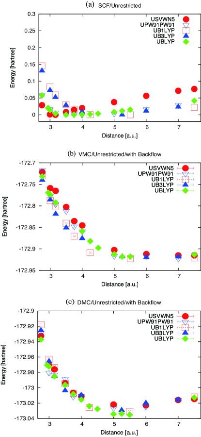
Figure 1: Binding curves obtained from unrestricted (a) SCF, (b) VMC, and (c) DMC calculations. In (a), SCF energies are shifted so that each minimum is set to be zero; the minimums are, $-172.758,-173.208,-173.026,-172.946$, and $-173.026$ hartree for SVWN5, PW91PW91, BLYP, B1LYP, B3LYP, respectively. In (b) and (c) error bars are within symbol size. VMC and DMC include the backflow transformation.

Binding curves obtained from SCF and QMC calculations using unrestricted SD wavefunctions are shown in Fig. 1 (a) - (c). At the SCF level, LDA (USVWN5) and GGA(UPW91PW91 and UBLYP) recover a bond length, $R_{e}$, near to the experimental value, 3.1748 [a.u.]Furche_Perdew_2006 , while the other hybrid functionals give a longer $R_{e}$. At the QMC level, using any of the XC functionals, however, the bond length, $R_{e}$, is very similar and much overestimated compared to experiment. The results imply that the non-local HF exchange favors a longer $R_{e}$. QMC essentially takes the non-local exchange into account even if the trial/guiding wavefunction is constructed without the HF exchange. VMC gives a quite shallow bottom of the binding curve, while DMC gets the curve recovered deeper. However, DMC still unsatisfactorily recovers about 30$\%$ of the experimental binding energy $D_{e}$, 0.0541 hartreeFurche_Perdew_2006 .

At the experimental $R_{e}$ some of the SCF calculations give lower molecular energies than twice the isolated atomic energies (zero-binding energies shown in Table 3), as shown in Table 2. LDA(USVWN5) and GGA(UPW91PW91) recover 164.5 % and 70.3 % of the experimental $D_{e}$, respectively, while UB3LYP gives 3.7 %. Underlined values in Table 2 highlight those lower than the zero-binding energies, which means that the molecule is bound at the experimental $R_{e}$. For example, RB3LYP-SCF does not bind the molecule, which is consistent with previous works Edgecombe_Becke_1995 ; Kitagawa_etal_2007 . To compare the atomic and molecular energies, the same basis sets and pseudopotentials were used. The RHF, UHF, and QMC calculations using the RHF and UHF trial wavefunctions were obtained by GAMESS/QWalk while the others are by Gaussian03/CASINO. A lower DFT-SCF energy does not mean a better description of the total energy because it does not necessarily satisfy the variational principle, while a lower QMC energy implies a solution closer to the exact one because of its variational property of the total energy. In Table 2, therefore, only the best (lowest) zero-binding energies of VMC and DMC using the B1LYP trial/guiding wavefunction are shown. Hence none of the QMC calculations at the SD level can reproduce a bound state at the experimental $R_{e}$.

It is worth noting in Table 2 that RHF gives a lower DMC energy than UHF. At the SCF level, in turn, RHF gives a much higher energy than any other, supporting the consensus that restricted treatments cannot well describe the localized amplitude of the wavefunction at ionic sites of a spin polarized system SZA89 . In DMC, however, the amplitude of the many-body wavefunction is automatically adjusted by the projection operation and is not directly governed by the XC approximation. The results show that the RHF nodal surface is superior to the UHF one, leading us to examine restricted methods for the generation of the trial nodal surface.

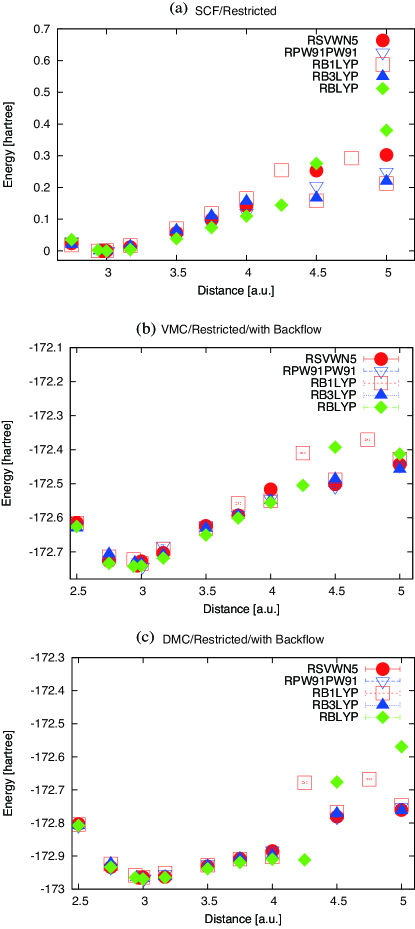
Figure 2: Binding curves obtained from restricted (a) SCF, (b) VMC, and (c) DMC calculations. In (a), SCF energies are shifted so that each minimum is set to be zero; the minimums are, $-172.753,-173.180,-173.004,-172.794$, and $-172.900$ hartree for SVWN5, PW91PW91, BLYP, B1LYP, B3LYP, respectively. In (b) and (c) error bars within symbol size. VMC and DMC include the backflow transformation.

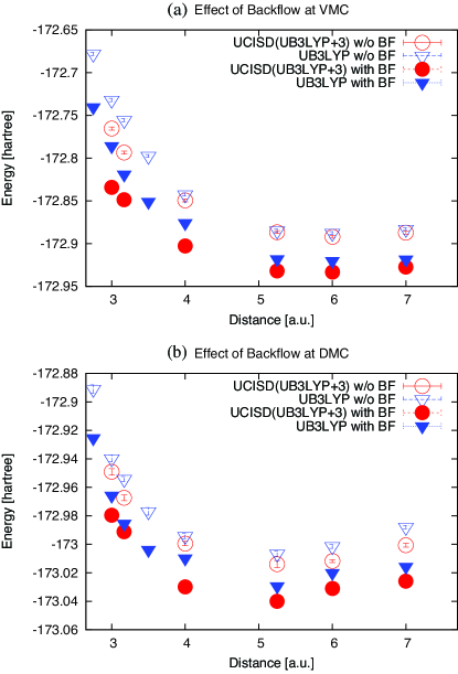
Figure 8: Comparison between results with and without the backflow transformation for (a) VMC and (b) DMC.

Figure 2 (a) - (c) shows binding curves evaluated by restricted methods. At the SCF level, they well reproduce the experimental $R_{e}$. A quite deep well bottom gives rise to an overestimate of $D_{e}$, which is attributed to a well-known failure of restricted methods SZA89 . Such an overestimate is modestly improved in DMC because the imaginary projection relaxes the many-body wavefunction at larger distances. From the viewpoint of evaluating $R_{e}$, RB3LYP gives the best restricted fixed nodes, though it is found to be variationally worse than any of unrestricted nodes. The variationally optimal fixed nodes within the SD approximation are obtained from UB3LYP, though it overestimates $R_{e}$ by around 50 % and underestimates $D_{e}$ by 30 %. The backflow transformation improves the ground state energy, but makes no significant improvements on $R_{e}$ and $D_{e}$, as shown in Fig. 8 (a) and (b).

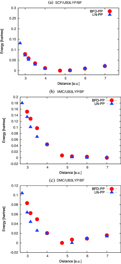
Figure 3: Comparison of binding curves using different pseudopotentials with UB3LYP/BF for (a) SCF, (b) VMC, and (c) DMC calculations. Energies are shifted so that each minimum to be zero: the values of the minimum are (a) $-173.026$ hartree for LN and $-173.849$ hartree for BFD, (b) $-172.920$ hartree for LN and $-173.746$ hartree for BFD, and (c) $-173.029$ hartree for LN and $-173.844$ hartree for BFD.

We also investigated the dependence on pseudopotentials for the best fixed nodes within the SD approximation, i.e., we performed UB3LYP-QMC with backflow for two different potentials, LN and BFD. The latter uses a contracted Gaussian basis set (33s29p19d2f)/ $\left[{\rm 5s5p4d2f}\right]$BUR08 . Though both pseudopotentials have the same effective valence electrons, the atomic energies are quite different from each other, as shown in Table 4 in terms of zero-binding energies. We note that considerably faster SCF convergence is observed with BFD, by a factor of five faster than LN, while the QMC statistical qualities (statistical noise, auto-correlation, and population fluctuation) are almost the same for both potentials. The LN/UB3LYP-SCF calculation gives a weak binding at the experimental $R_{e}$, but such a bound state disappears for BFD/UB3LYP-SCF (unbound), as seen in Table 4. Comparisons of binding curves are shown in Fig. 3 (a) - (c). There is no significant difference between LN and BFD in the predictions of $R_{e}$ and $D_{e}$, though BFD slightly underestimates $D_{e}$ and overestimates $R_{e}$. In summary, this result may justify our choice of the LN pseudopotential.

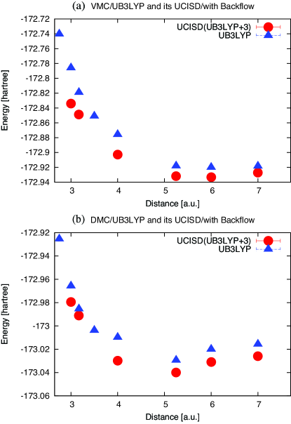
Figure 7: Comparison of QMC binding curves using the UB3LYP-SD and UCISD(UB3LYP+3) trial/guiding wavefunctions for (a) VMC and (b) DMC with the backflow transformation.

The time step dependence of the DMC energies is shown in Fig. 4. It is confirmed that the result with $dt=0.01$ agrees with the results using other choices of $dt$ to within one standard deviation $\sigma$. The sudden decrease in the energy at $dt=0.001$ is found to be similar to Fig. 7 of Ref. UMR93 .

III.2 Restricted multi determinant calculations

Valence bond (VB) type many-body wavefunctions are expected to give a proper description of the spin polarized Cr₂BAU80a with a compact form of the MD expansion. Generalized VB (GVB) SCF is available in GAMESSGAM93 and we can use GVB orbitals to generate QMC trial/guiding wavefunctions. Table 5 shows the symmetries of the UHF natural orbitals (NO) near the HOMO-LUMO level. We considered 12 active occupied molecular orbitals up to level 20, which arises from the 4s(1)3d(5) atomic orbitals. The GVB function is formed as

$$\Psi_{\rm GVB}^{\left(6\right)}={\hat{A}}\left\{{\Phi_{\rm core}^{\left(8\right)}\cdot\prod\limits_{p=1}^{6}{\Phi_{{\rm GVB};p}^{\left(2\right)}}}\right\}\ ,$$ (5)

where $\hat{A}$ denotes an antisymmetrizer and $\Phi_{\rm core}^{\left(8\right)}$ the core contribution. $\Phi_{{\rm GVB};p}^{\left(2\right)}$ consists of the (GVB) orbital pairs, for which each of $j$-occupied orbitals ($j\in\left\{{9,\cdots,14}\right\}$) in the active space is paired with a virtual orbital with the same symmetry. Hence the following six pairs are involved: $p=(10,19),(11,18),(14,15),(13,16),(12,17)$, and $(9,20)$. The orbitals in the active space were optimized by a SCF procedure with respect to $\Psi_{\rm GVB}^{\left(6\right)}$. An explicit form of $\Psi_{\rm GVB}^{\left(6\right)}$ takes a restricted CI expansion, $D_{j}^{\uparrow}=D_{j}^{\downarrow}$, $c_{ij}=c_{i}\cdot\delta_{ij}$, as,

$$F_{\rm AS}^{\rm GVB}=\sum_{i=0}^{63}{c_{i}\cdot D_{i}^{\sigma}}=\left[\begin{array}[]{l}\left({g_{9}\cdot\hat{1}+e_{9}\cdot\hat{P}_{9\to S_{9}}}\right)\\ \otimes\left({g_{10}\cdot\hat{1}+e_{10}\cdot\hat{P}_{10\to S_{10}}}\right)\\ \otimes\cdots\\ \otimes\left({g_{14}\cdot\hat{1}+e_{14}\cdot\hat{P}_{14\to S_{14}}}\right)\\ \end{array}\right]\cdot D_{0}^{\sigma}\ ,$$ (6)

where $g_{j}$ and $e_{j}$ are coefficients such that $c_{0}=g_{9}\cdot g_{10}\cdots g_{14}\,$ etc. $S_{j}$ denotes the index of a virtual orbital with the same symmetry as the $j$-occupied orbital. The operators, $\hat{1}$ and $\hat{P}_{j\to S_{j}}$, are the identity and permutation operators, respectively. $\hat{P}_{j\to S_{j}}$ swaps the $j$-occupied orbital in $D_{0}^{\sigma}$ into the $S_{j}$-virtual one. As discussed later a usual CI treatment in a quantum chemistry code gives hundreds of thousands of terms in the expansion, all of which can not be included in a QMC calculation. GVB provides, in contrast, a very compact form of the MD expansion with only 64 terms.

Starting with UHF-NO and optimizing the coefficients, $g_{j}$ and $e_{j}$, as well as the orbitals, GVB-SCF gives a variationally better description than RHF within a restricted SCF treatment, as seen in Table 6. With the coefficients given by GVB-SCF, the wavefunction achieves a better (lower) energy than HF at the VMC level, but it turns out to be higher than HF using DMC (the row of ’GVB(6)’ in Table 6). Then we tried to optimize the coefficients further by VMC. A total of 64 coefficients can be reduced to 48 independent variables by its symmetry. We adopted a mixed scheme between energy and variance minimization UMR05 with 95% weight on the former. Even though we ignore the above symmetry reduction to optimize 64 parameters independently, the optimized values of the parameters roughly satisfy their symmetries. Using the GVB nodes with these coefficients, we obtained a better DMC value than when using the HF nodes, but still above the zero-binding energy (the row of ’GVB(6)opt’ in Table 6).

Next we considered a restricted CASSCF node ($D_{j}^{\uparrow}=D_{j}^{\downarrow}$, $c_{ij}=c_{i}\cdot\delta_{ij}$), having the form of

$$F_{\rm AS}^{\rm CAS}=\sum_{i=0}^{N_{\rm CAS}-1}{c_{i}\cdot D_{i}^{\sigma}}=\sum_{i=0}^{N_{\rm CAS}-1}{c_{i}\cdot\hat{P}_{l\rightarrow m}^{\left(i\right)}D_{0}^{\sigma}}\ .$$ (7)

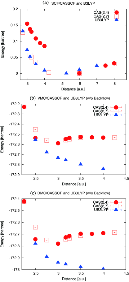
Figure 5: (a) SCF, (b) VMC, and (c) DMC binding curves using the CASSCF(2,4), CASSCF(2,7), and UB3LYP (trial) wavefunctions. In (a) SCF energies are shifted so that each minimum, $-171.540,-171.461$, and $-173.026$ hartree to be zero. In (b) and (c) error bars are within symbol size.

An initial guess for the orbitals was taken from a UHF-NO calculation and optimized self-consistently with respect to the above many-body wavefunction. We employed (restricted) CASSCF(2,4) and CASSCF(2,7) methods, in which the number of expansion terms amounts to $N_{\rm CAS}$=16 and 49, respectively. The results are shown in Fig. 5 (a) - (c). Though they could not achieve a variationally lower energy than UB3LYP-SD in terms of the final DMC energy, several interesting behaviors are found as follows: CASSCF(2,7)-SCF gives a binding curve with a similar shape to UB3LYP-SCF, though overestimating $R_{e}$. At the QMC level, in turn, the evaluated value of $R_{e}$ gets shorter, and the shape of the binding curve is similar to the restricted SD cases. This implies that the terms in the MD expansion well describe the localized amplitude as that obtained from the unrestricted SD cases, but the nodal structure is essentially the same as that obtained from the restricted SD. In order to obtain a variationally lower energy we have tried a restricted MRCI (multi reference CI) using orbitals obtained from the present CASSCF calculation, but QMC calculations using the MRCI trial/guiding wavefunction could not give better results than when using the UB3LYP-SD one.

III.3 Unrestricted multi determinant calculations

Several advanced MD implementations such as CASSCF are available at the restricted level, but we could not obtain better results than UB3LYP-SD. We therefore tried unrestricted CI (UCI) methods, for which Gaussian03 Gaussian03 was used to provide UCISD (UCI singles and doubles). Using a UHF reference, the UCI expansion gives 7,521,823 terms, all of which can not be taken into account in a QMC calculation. We truncated this expression into 35 determinants, removing those terms with coefficients $\left|c_{i}\right|<0.01$. The expansion coefficients were optimized further by VMC, first by weight-limitted variance minimizations CASINO , followed by energy minimizations. The results at the experimental $R_{e}$ are shown in Table 7. At the SCF level, UCISD achieved a lower energy than its initial guess UHF, implying that the coefficients are well optimized by CI-SCF. UCISD gives a higher energy than UB3LYP at the SCF level, which does not matter, because there is no variational relation between them. Using the UCISD trial wavefunction, we achieved a lower VMC energy than when using the UB3LYP one, indicating that our VMC optimization of the CI coefficients was successful. At DMC, however, UCISD turned out to give a worse result than UB3LYP. We also tried another choice of expansion: 67 excited configurations, in which the active space was HOMO$\pm$6 and the single and double excitations of occupied orbitals were restricted to virtual orbitals with the same symmetry. This choice gives, however, a worse result than UB3LYP-SD even at the VMC level [-172.744(2) hartree].

The above CI treatments could not give any variationally better trial node than UB3LYP-SD. The easiest way to go beyond those treatments would be to add UCI expansions to UB3LYP-SD because it is the best starting point. By considering the UB3LYP orbital symmetry near the HOMO level, we made two different sizes of CI expansions: The first one took into account only 3 virtual orbitals above the LUMO, including only $\sigma$ and $\pi$ symmetries [for which we refer it as UCISD(UB3LYP+3)], and the second was a larger one with 10 virtual orbitals in which $\sigma$, $\pi$, and $\delta$ symmetries were included [UCISD(UB3LYP+10)]. In both cases we considered only such excited configurations between the orbitals with the same symmetry, resulting in around 50 and 650 determinants for UCISD(UB3LYP+3) and UCISD(UB3LYP+10), respectively (the numbers of determinants vary a little amount depending on $R$).

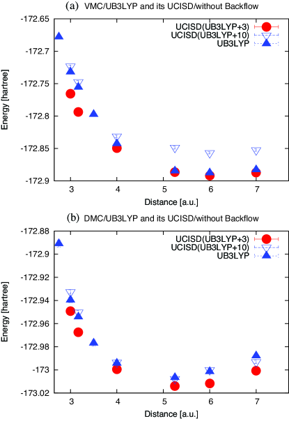
Figure 6: Comparison of QMC binding curves using the UB3LYP-SD and UCISD(UB3LYP+$N$) ($N=3,10$) trial/guiding wavefunctions for (a) VMC and (b) DMC without Backflow transformation.

The results are shown in Fig. 6 (a) and (b). As seen in Fig. 6 (a), VMC using the UCISD(UB3LYP+3) trial wavefunction gives a better result than when using the UB3LYP-SD one, because the former includes more variational degrees of freedom to be optimized. For UCISD(UB3LYP+10), however, we could not get a satisfactory optimization, giving a higher energy than the initial UB3LYP-SD calculation. Nevertheless the DMC calculation with the UCISD(UB3LYP+10) node gives a slightly lower energy than that with the UB3LYP node (Fig. 6 (b)). It is apparent that the UCISD(UB3LYP+3) node give a lower DMC energy than the UB3LYP-SD node. Focussing on UCISD(UB3LYP+3), we further introduced the backflow transformation, getting the best binding curve beyond SD, as shown in Fig. 7 (a) and (b). Similar to the SD cases, the DMC projection gets $R_{e}$ shorter and $D_{e}$ deeper than VMC. Though UCISD(UB3LYP+3) gives a variationally better result than any SD treatment, it could not hardly improve the binding nature, i.e., it overestimates $R_{e}$ and underestimates $D_{e}$, compared with the experimental values. As seen in Fig. 8 (a) and (b), the backflow does not improves these as well.

IV Concluding Remarks

We studied the binding curve of the ground state Cr₂ dimer using the fixed node DMC method. Various different types of nodal structures were compared based on the variational principle with respect to the node of the DMC guiding function. We tested several choices of XC functionals with or without spin restriction on the orbital functions composing the many-body wavefunction. We also tried computationally expensive choices of UCI expansions with backflow transformation.

Within the SD treatment, UB3LYP turns out to give the variationally best trial node. Except HF, the unrestricted nodes are found to be better than the restricted ones. Any choice gives binding curves with a energy minimum, but for unrestricted trial nodes they end up with a much larger $R_{e}$ and smaller $D_{e}$ in the QMC final results, compared with the experimental values. Though some unrestricted DFT-SCF calculations, such as ULDA and UGGA, reproduce a proper $R_{e}$, it is found that the QMC calculations with these trial nodes overestimate $R_{e}$. The restricted nodes recover fairly well $R_{e}$ even at QMC, but they give a higher energy than the unrestricted ones. At the experimental $R_{e}$, we could not get a stable molecular energy lower than twice the atomic energy at the QMC level, although some DFT-SCF calculations did reproduce a bound state.

We also examined whether the binding curve could be improved by different pseudopotentials, comparing the BFD potential with the LN one. Both potentials give almost the same binding curve, which justifies our choice of pseudopotentials. The time step bias is confirmed to be kept within the error bar considered in this study. The backflow transformation turned out to give no specific improvements on describing the binding nature, although it did improve the energy variationally.

Within the framework of the MD approximation, we first tried the GVB model as a compact expansion for the many-body wavefunction because of its plausible physical meaning. Starting with HF orbitals, we optimized the GVB orbitals and coefficients by a SCF procedure, but it could not give a better result than the unrestricted SD in the DMC final results, probably because the restricted treatment has a limitation in describing the spin polarized nature in Cr₂. We also run DMC using the trial nodes derived from a restricted MD expansion with orbitals optimized by CASSCF, but it ends up with a worse QMC result than the unrestricted DFT-SD nodes. Though the restricted CASSCF itself gives a too large $R_{e}$ similar to the unrestricted DFT calculations, the QMC calculations with the CASSCF nodes give properly shorten $R_{e}$ near to the experimental value. Then we decided to use the unrestricted CI nodes. First, we chose such excited configurations as those with a large coefficient weight and re-optimized the coefficients. VMC with this trial wavefunction gives a lower energy than that with the UB3LYP one. On the other hand, the corresponding DMC calculation gives a higher energy than DMC using the UB3LYP nodes. Next, we manually constructed a UCI expansion with UB3LYP orbitals and optimized their coefficients. Though the UCI-MD node gives a better DMC result than the UB3LYP-SD one, it gives no improvements on the binding natures, i.e., it still overestimates $R_{e}$ and underestimate $D_{e}$.

V Acknowledgments

The authors would like to thank Prof. Lubos Mitas for introducing this work to us and for providing basis sets and pseudopotentials, Dr. Lucas Wagner for his help about the QWalk code, Ms. Kaoru Nishi for her work on the numerical data, and Dr. Mark A. Watson for his fruitful comments. The computation in this work has been partially performed using the facilities of the Center for Information Science in JAIST. K.H. is grateful for a JSPS Postdoctoral Fellowship for Research Abroad. Financial support was provided by Precursory Research for Embryonic Science and Technology, Japan Science and Technology Agency (PRESTO-JST), and by a Grant–in–Aid for Scientific Research in Priority Areas ”Development of New Quantum Simulators and Quantum Design (No. 17064016)” (Japanese Ministry of Education,Culture, Sports, Science, and Technology ; KAKENHI-MEXT) for R.M.

Appendix A Jastrow functions

In CASINO CASINO , $u$, $\chi$, and $f$ terms in Eq. (4) are given in power expansion form as DRU04

$$u\left({r_{ij}}\right) = \left({r_{ij}-L_{u}}\right)^{C}\times\Theta\left({L_{u}-r_{ij}}\right)$$ (8)

$$\times\left({\alpha_{0}+\left[{\frac{{\Gamma_{ij}}}{{\left({-L_{u}}\right)^{C}}}+\frac{{\alpha_{0}C}}{{L_{u}}}}\right]r_{ij}+\sum\limits_{l=2}^{N_{u}}{\alpha_{l}}r_{ij}^{l}}\right)\ ,$$

$$\chi_{I}\left({r_{iI}}\right) = \left({r_{iI}-L_{\chi I}}\right)^{C}\times\Theta\left({L_{\chi I}-r_{iI}}\right)$$ (9)

$$\times\left({\beta_{0I}+\left[{\frac{{-Z_{I}}}{{\left({-L_{\chi I}}\right)^{C}}}+\frac{{\beta_{0I}C}}{{L_{\chi I}I}}}\right]r_{iI}+\sum\limits_{m=2}^{N_{\chi}}{\beta_{mI}}r_{{}_{iI}}^{m}}\right)\ ,$$

$$f_{I}\left({r_{iI},r_{jI},r_{ij}}\right) = \left({r_{iI}-L_{fI}}\right)^{C}\left({r_{jI}-L_{fI}}\right)^{C}$$ (10)

$$\times\Theta\left({L_{fI}-r_{iI}}\right)\Theta\left({L_{fI}-r_{jI}}\right)\sum\limits_{l=0}^{N_{fI}^{eN}}{\sum\limits_{m=0}^{N_{fI}^{eN}}{\sum\limits_{n=0}^{N_{fI}^{ee}}{\gamma_{lmnI}r_{iI}^{l}r_{jI}^{m}r_{ij}^{n}}}}\ .$$

In QWalk QWA09 , instead, the terms are expanded with basis sets $\left\{{b_{j}\left(r\right)}\right\}$ which vanish at some cutoff length , given as

$$u\left({r_{ij}}\right) = u_{0}\left({r_{ij}}\right)+\sum\limits_{m=1}^{M_{u}}{c_{m}\cdot b_{m}^{\left({ee}\right)}\left({r_{ij}}\right)}\ ,$$ (11)

$$\chi_{I}\left({r_{iI}}\right) = \sum\limits_{m=1}^{M_{\chi}}{c_{m}\cdot b_{m}^{\left({eI}\right)}\left({r_{iI}}\right)}\ ,$$ (12)

$$f_{I}\left({r_{iI},r_{jI},r_{ij}}\right) = \sum\limits_{\left\langle{k,m,n}\right\rangle}{c_{kmn}\cdot b_{m}^{\left({eI}\right)}\left({r_{iI}}\right)b_{n}^{\left({eI}\right)}\left({r_{jI}}\right)\cdot b_{k}^{\left({ee}\right)}\left({r_{ij}}\right)}\ ,$$ (13)

with

$$u_{0}\left(r\right) = \frac{1}{4}\cdot\frac{{p_{\uparrow\uparrow}\left(r\right)}}{{1+\underline{\gamma_{\uparrow\uparrow}}\cdot p_{\uparrow\uparrow}\left(r\right)}}\cdot\hat{P}_{\uparrow\uparrow}+\frac{1}{2}\cdot\frac{{p_{\uparrow\downarrow}\left(r\right)}}{{1+\underline{\gamma_{\uparrow\downarrow}}\cdot p_{\uparrow\downarrow}\left(r\right)}}\cdot\hat{P}_{\uparrow\downarrow}\ ,$$ (14)

$$p_{\sigma\sigma^{\prime}}\left(r\right) = \left({\frac{r}{{r_{c}^{\sigma\sigma^{\prime}}}}}\right)-\left({\frac{r}{{r_{c}^{\sigma\sigma^{\prime}}}}}\right)^{2}+\frac{1}{3}\left({\frac{r}{{r_{c}^{\sigma\sigma^{\prime}}}}}\right)^{3}\ ,$$ (15)

$$b_{m}^{\left({pq}\right)}\left(r\right) = \frac{{1-z^{\left({pq}\right)}\left(r\right)}}{{1+\beta_{m}^{\left({pq}\right)}\cdot z^{\left({pq}\right)}\left(r\right)}}\ ,$$ (16)

$$z^{\left({pq}\right)}\left(r\right) = \left({\frac{r}{{b_{0}^{\left({pq}\right)}}}}\right)^{2}\left[{6-8\left({\frac{r}{{b_{0}^{\left({pq}\right)}}}}\right)+3\left({\frac{r}{{b_{0}^{\left({pq}\right)}}}}\right)^{2}}\right]\ ,$$ (17)

where the upper index $\left(pq\right)$ in Eqs. 16 and 17 stands for particle pairs such as $\left(eI\right)$ or $\left(ee\right)$. The term $u_{0}$ imposes the electron-electron cusp condition for spin pair $\sigma\sigma^{\prime}$ with a projection operator $\hat{P}_{\sigma\sigma^{\prime}}$ and cutoff length $r_{c}^{\sigma\sigma^{\prime}}$. The Poly-Pade type basis $b_{m}^{\left({pq}\right)}$ with $z^{\left({pq}\right)}\left(r\right)$ is designed to be cutoff quadratically at $b_{0}^{\left({pq}\right)}$. The parameters $\left\{\beta_{m}^{\left({pq}\right)}\right\}$ are generated from a given $\beta_{0}^{\left({pq}\right)}$ using the following recursions:

$$\beta_{1} = \exp\left({1.6}\right)\times\left({1+\beta_{0}}\right)\ ,$$ (18)

$$\beta_{k} = \left[{\exp\left({1.6}\right)}\right]\times\beta_{k-1}\quad\left(k>1\right)\ .$$ (19)

The range of summation for the $f$-term, $\left\langle{k,m,n}\right\rangle$, denotes the pairs specified according to a given order $\left(M_{u},M_{\chi}\right)$. For the present work $\left(M_{u},M_{\chi}\right)=\left(3,3\right)$ amounts to 12 terms for the expansion.

For CASINO we used expansion orders of $N_{\rm u}$=8, $N_{\rm\chi}$=8, $N_{\rm fI}^{eN}$=2, and $N_{\rm fI}^{ee}$=2, with fixed cutoff lengths $L_{\rm u}$ = 5 [a.u.], $L_{\rm\chi}$ = 4 [a.u.], and $L_{\rm fI}$ = 3[a.u.], respectively. In QWalk we choose cutoff lengths to be fixed as 7.5 [a.u.].

Figure 4: Time step dependence of ground state energy in the DMC calculation with the backflow transformation. The fixed node is generated from the UB3LYP-DFT calculation.

Table 1: Exchange-Correlation potentials. ‘GC’ stands for gradient correction.

	Exchange			Correlation
	Non-local	Local	GC	Local	GC
Functional	$V_{\rm X}^{\rm HF}$[$\%$]	$V_{\rm X}^{\rm Slater}$[$\%$]	$\delta V_{\rm X}$ [$\%$]	$V_{\rm C}^{\rm VWN5}$[$\%$]	$\delta V_{\rm C}$ [$\%$]
SVWN5	0	100	0	100	0
PW91PW91	0	100	100 ​PW91	100	100 ​PW91
BLYP	0	100	100 ​B88	100	100 ​LYP
B1LYP	25	75	75 ​B88	100	100 ​LYP
B3LYP	20	80	72 ​B88	100	81 ​LYP

Table 2: Ground state energies [hartree] at the experimental bond length. Underlined values highlight those lower than the zero-binding energy in Table 3.

	SCF	VMC	DMC
UHF	-171.701	-172.665(6)	-172.903(2)
RHF	-171.097	-172.584(4)	-172.911(2)
USVWN5	-172.757	-172.765(2)	-172.976(2)
RSVWN5	-172.741	-172.704(2)	-172.963(3)
UPW91PW91	-173.201	-172.796(2)	-172.983(2)
RPW91PW91	-173.173	-172.681(2)	-172.954(2)
UBLYP	-173.022	-172.792(2)	-172.985(2)
RBLYP	-173.000	-172.719(2)	172.965(1)
UB1LYP	-172.887	-172.800(2)	-172.974(3)
RB1LYP	-172.777	-172.692(2)	-172.952(2)
UB3LYP(without BF)	-172.974	-172.756(2)	-172.954(2)
UB3LYP(with BF)	-172.974	-172.819(2)	-172.985(2)
RB3LYP	-172.885	-172.710(2)	-172.963(2)
ZeroBinding(Best)		-172.931(2)	-173.012(3)

Table 3: Zero-binding energies [hartree] for different trial wavefunctions. QMC values are evaluated with the backflow transformation.

	SCF	VMC	DMC
SVWN5	-172.668	-172.918(2)	-173.007(1)
PW91PW91	-173.163	-172.919(2)	-173.007(1)
BLYP	-172.972	-172.925(2)	-173.008(2)
B1LYP	-172.913	-172.931(2)	-173.012(3)
B3LYP	-172.972	-172.910(2)	-173.000(2)
HF	-171.875	-172.921(2)	-173.002(2)

Table 4: Comparison of zero-binding energies [hartree] for different pseudopotentials. SCF molecular energies are also listed for comparison, designated as SCF (molecule).

pseudopotentials	SCF	SCF (molecule)	VMC	DMC
Lee-Needs (LN)	-172.972	-172.974	-172.910(2)	-173.000(2)
Burkatzki-Filippi-Dolg (BFD)	-173.809	-173.780	-173.740(2)	-173.820(2)

Table 5: Symmetries of the UHF natural orbitals near the HOMO (14) and LUMO (15) levels.

Level	Symmetry
20	$\sigma_{4s}$
19	$xz$
18	$yz$
17	$\sigma_{z^{2}}$
16	$xy$
15	$x^{2}-y^{2}$
14	$x^{2}-y^{2}$
13	$xy$
12	$\sigma_{z^{2}}$
11	$yz$
10	$xz$
9	$\sigma_{4s}$

Table 6: GVB energies [hartree] at experimental bond length. ‘GVB(6)opt’ stands for that with coefficients optimized further by VMC (see text).

Methods	SCF	VMC	DMC
UHF	-171.701	-172.665(6)	-172.903(2)
RHF	-171.097	-172.584(4)	-172.911(2)
GVB(6)	-171.624	-172.698(6)	-172.861(2)
GVB(6)opt		-172.723(2)	-172.933(2)

Table 7: Comparison between UCISD-MD and UB3LYP-SD at experimental bond length. QMC results are those without the backflow transformation. Underlined value highlights that reproducing the binding.

Methods	SCF	VMC	DMC
UHF	-171.701	-172.665(6)	-172.903(2)
UB3LYP(w/o BF)	-172.974	-172.756(2)	-172.954(2)
UCISD(w/o BF)	-172.599	-172.772(2)	-172.926(3)
ZeroBinding(Best)		-172.931(2)	-173.012(3)

References

- (1) D.L. Michalopoulos, M.E. Geusic, S.G. Hansen, D.E. Powers, and R.E. Smalley, J. Phys. Chem. 86, 3914 (1982).
- (2) V.E. Bondybey, and J.H. English, Chem. Phys. Lett. 50, 1451 (1983).
- (3) B. Simard, M.-A. Lebeault-Dorget, A. Marijnissen, and J.J. ter Meulen, J. Chem. Phys. 108, 9668 (1998).
- (4) K. Hilpert and K. Ruthardt, Ber. Bunsen-Ges. Phys. Chem. 91, 724 (1987).
- (5) C.-X. Su, D.A. Hales, and P.B. Armentrout, Chem. Phys. Lett. 201, 199 (1993).
- (6) S.M. Casey and D.G. Leopold, J. Phys. Chem. 97, 816 (1993).
- (7) M. Moskovits, W. Limm, and T. Mejean, J. Chem. Phys. 82, 4875 (1985).
- (8) K. Anderson, Chem. Phys. Lett. 237, 212 (1995).
- (9) A.D. McLean and B. Liu, Chem. Phys. Lett. 101, 144 (1983).
- (10) K.W. Richman and E.A. McCullough, Jr., J. Chem. Phys. 87, 5050 (1987).
- (11) S.P. Walch, C.W. Baushlicher, Jr., B.O. Roos, C.J. Nelin, Chem. Phys. Lett. 103, 175 (1983).
- (12) C. Wood, M. Doran, I.H. Hillier, and M.F. Guest, Faraday Symp. Chem. Soc. 14, 159 (1980).
- (13) M.M. Goodgame and W.A. Goddard, III, J. Phys. Chem. 85, 215 (1981).; M.M. Goodgame and W.A. Goddard, III, Phys. Rev. Lett. 48, 135 (1982).
- (14) M.M. Goodgame and W.A. Goddard, III, Phys. Rev. Lett. 54, 661 (1985); see also, B. Delly, Phys. Rev. Lett. 55, 2090.
- (15) P.M. Atha and I.H. Hillier, Mol. Phys. 45, 285 (1982).
- (16) R.A. Kok and M.B. Hall, J. Chem. Phys. 87, 715 (1983).
- (17) L. Visscher, H. DeRaedt, and W.C. Nieuwpoor, Chem. Phys. Lett. 227, 327 (1994).
- (18) H. Dachsel, J. Harrison, and D.A. Dixon, J. Phys. Chem. A 103, 152 (1999).
- (19) G.E. Scuseria, J Chem Phys 94, 442 (1991); see also, G.E. Scuseria and H.F. Schaefer, III, Chem. Phys. Lett. 174, 501 (1990).
- (20) C.W. Bauschlicher Jr., and H. Partridge, Chem. Phys. Lett. 231, 277 (1994).
- (21) T. Müller, J. Phys. Chem. A 113, 12729 (2009).
- (22) H. Stoll, H.-J. Werner, Mol. Phys. 88, 793 (1996).
- (23) K. Anderson, B.O. Roos, P.-Å. Malmqvist, and P.-O. Widmark, Chem. Phys. Lett. 230, 391 (1994).
- (24) K. Anderson and B.O. Roos, Chem. Phys. Lett. 245, 215 (1995).
- (25) K. Anderson, C.W. Baushlicher, Jr., B.J. Persson, B.O. Roos, Chem. Phys. Lett. 257, 238 (1996).
- (26) P. Celani, H. Stoll, H.-J. Werner, and P.J. Knowles, Mol. Phys. 102, 2369 (2004).
- (27) A.O. Mitrushenkov and P. Palmieri, Chem. Phys. Lett. 278, 285 (1997).
- (28) C. Angeli, R. Cimiraglia, and J.-P. Malrieu, J. Chem. Phys. 117, 9138 (2002).
- (29) C. Angeli, B. Bories, A. Cavallini, and R. Cimiraglia, J. Chem. Phys. 124, 054108 (2006).
- (30) Y. Takahara, K. Yamaguchi, and T. Fueno, Chem. Phys. Lett. 158, 95 (1989).
- (31) G. Moritz, B.A. Hess, and M. Reiher, J. Chem. Phys. 122, 024107 (2005).
- (32) Y. Kurashige and T. Yanai, J. Chem. Phys. 130, 234114 (2009).
- (33) B. Delley, A.J. Freeman, and D.E. Ellis, Phys. Rev. Lett. 50, 488 (1983).
- (34) J. Bernholc and N.A.W. Holzwarth, Phys. Rev. Lett. 50, 1451 (1983).
- (35) B.I. Dunlap, Phys. Rev. A 27, 2217 (1983).
- (36) N.A. Baykara, B.N. McMaster, and D.R. Salahub, Mol Phys 52, 891 (1984).
- (37) G.S. Painter, J. Phys. Chem. 90, 5530 (1986).
- (38) K.E. Edgecombe and A.D. Becke, Chem. Phys. Lett. 244, 427 (1995).
- (39) H. Cheng and L.S. Wang, Phys. Rev. Lett. 77, 51 (1996).
- (40) E.J. Thomas, III, J.S. Murray, C.J. O’Connor, and P. Politzer, J. Mol. Struct. (Theochem) 487, 177 (1999).
- (41) N. Desmarais, F.A. Reuse, and S.N. Khanna, J. Chem. Phys. 112, 5576 (2000).
- (42) S. Yanagisawa, T. Tsuneda, and K. Hirao, J. Chem. Phys. 112, 545 (2000).
- (43) C.J. Barden, J.C. Rienstra-Kiracofe, and H.F. Schaefer, III, J. Chem. Phys. 113, 690 (2000).
- (44) M. Valiev, E.J. Bylaska, J.H. Weare, J. Chem. Phys. 119, 5955 (2003).
- (45) G.L. Gutsev and C.W. Bauschlicher, Jr., J. Phys. Chem. A 107, 4755 (2003).
- (46) F. Furche and J.P. Perdew, J. Chem. Phys. 124, 044103 (2006).
- (47) P. Calaminici, F. Janetzko, A.M. Köster, R. Mejia-Olvera, and B. Zuniga-Gutierrez, J. Chem. Phys. 126, 044108 (2007).
- (48) Y. Kitagawa, T. Saito, M. Ito, M. Shoji, K. Koizumi, S. Yamanaka, T. Kawakami, M. Okamura, and K. Yamaguchi, Chem. Phys. Lett. 442, 445 (2007); see also, Y. Kitagawa, T.Kawakami, T. Saito, T. Kawakami, M. Okamura, and K. Yamaguchi, Int. J. Quantum Chem. 109, 3315 (2009).
- (49) Y. Shi-Ying, Chinese Phys. B 17, 2925 (2008).
- (50) T. Tsuchimochi, G.E. Scuseria, and A. Savin, J. Chem. Phys. 132, 024111 (2010).
- (51) Hammond, B.L.; Lester, W.A., Jr.; Reynolds, P.J. Monte Carlo Methods in Ab Initio Quantum Chemistry; World Scientific: Singapore, 1994.
- (52) Foulkes, W.M.C.; Mitas, L.; Needs, R.J.; Rajagopal, G. Rev Mod Phys 2001, 73, 33.
- (53) D.M. Ceperley, J. Stat. Phys. 63 (1991) 1237.
- (54) L. Wagner, L. Mitas, Chem. Phys. Lett. 370, 412 (2003).
- (55) R. J. Jastrow, Phys. Rev. 98, 1479 (1955).
- (56) Y. Lee (private communication); see also Y. Lee, P. R. C. Kent, M. D. Towler, R. J. Needs, and G. Rajagopal, Phys. Rev. B 62, 13347 (2000) for large-core version of these pseudopotentials.
- (57) M. Burkatzki, C. Filippi, M. Dolg in J. Chem. Phys. 129, 164115 (2008).
- (58) Gaussian 03, Revision E.01, M. J. Frisch, G. W. Trucks, H. B. Schlegel, G. E. Scuseria, M. A. Robb, J. R. Cheeseman, J. A. Montgomery, Jr., T. Vreven, K. N. Kudin, J. C. Burant, J. M. Millam, S. S. Iyengar, J. Tomasi, V. Barone, B. Mennucci, M. Cossi, G. Scalmani, N. Rega, G. A. Petersson, H. Nakatsuji, M. Hada, M. Ehara, K. Toyota, R. Fukuda, J. Hasegawa, M. Ishida, T. Nakajima, Y. Honda, O. Kitao, H. Nakai, M. Klene, X. Li, J. E. Knox, H. P. Hratchian, J. B. Cross, V. Bakken, C. Adamo, J. Jaramillo, R. Gomperts, R. E. Stratmann, O. Yazyev, A. J. Austin, R. Cammi, C. Pomelli, J. W. Ochterski, P. Y. Ayala, K. Morokuma, G. A. Voth, P. Salvador, J. J. Dannenberg, V. G. Zakrzewski, S. Dapprich, A. D. Daniels, M. C. Strain, O. Farkas, D. K. Malick, A. D. Rabuck, K. Raghavachari, J. B. Foresman, J. V. Ortiz, Q. Cui, A. G. Baboul, S. Clifford, J. Cioslowski, B. B. Stefanov, G. Liu, A. Liashenko, P. Piskorz, I. Komaromi, R. L. Martin, D. J. Fox, T. Keith, M. A. Al-Laham, C. Y. Peng, A. Nanayakkara, M. Challacombe, P. M. W. Gill, B. Johnson, W. Chen, M. W. Wong, C. Gonzalez, and J. A. Pople, Gaussian, Inc., Wallingford CT (2004).
- (59) R. J. Needs, M. D. Towler, N. D. Drummond and P. Lopez Rios, J. Phys.: Condens. Matter 22, 023201 (2010).
- (60) M.W. Schmidt, K.K. Baldridge, J.A. Boatz, S.T. Elbert, M.S. Gordon, J.H. Jensen, S. Koseki, N. Matsunaga, K.A. Nguyen, S.J. Su, T.L. Windus, M. Dupuis, J.A. Montgomery, J. Comput. Chem. 14, 1347 (1993).
- (61) Lucas K. Wagner, Michal Bajdich, and Lubos Mitas, J. Comput. Phys., 228, 3390 (2009).
- (62) N. D. Drummond, M. D. Towler and R. J. Needs, Phys. Rev. B 70, 235119 (2004).
- (63) T. Kato, Commun. Pure Appl. Math. 10, 151 (1957).
- (64) N. D. Drummond and R. J. Needs, Phys. Rev. B 72, 085124 (2005).
- (65) C. J. Umrigar and C. Filippi, Phys. Rev. Lett. 94, 150201 (2005).
- (66) R. P. Feynman and M. Cohen, Phys. Rev. Lett. 102, 1189 (1956).
- (67) N. D. Drummond, P. L. Rios, A. Ma, J. R. Trail, G. G. Spink, M. D. Towler and R. J. Needs, J. Phys. Chem. 124, 224104 (2006).
- (68) P. López Rios, A. Ma, N. D. Drummond, M. D. Towler and R. J. Needs, Phys. Rev. E 74, 066701 (2006).
- (69) A. Szabo and N. S. Ostlund, ”Modern Quantum Chemistry”, McGraw-Hill, New York (1989).
- (70) M. Casula, Phys. Rev. B 74, 161102 (2006).
- (71) C. W. Bauschlicher, Jr., J. Chem. Phys. 72(2), 880 (1980).
- (72) C.J. Umrigar, M.P. Nightingale, and K.J. Runge, J. Chem. Phys. 99, 2865 (1993).
- (73) L. Mitas, E.L. Shirley, D.M. Ceperley, J Chem Phys 95, 3467 (1991).
- (74) M. Bajdich, L. Mitas, G. Drobn, L. K. Wagner and K. E. Schmidt. Phys. Rev. Lett. 96, 130201 (2006).
- (75) C.J. Umrigar and C. Filippi, Phys. Rev. Lett. 94, 150201 (2005).