Optimal stopping for the predictive maintenance of a structure subject to corrosion

Abstract

We present a numerical method to compute the optimal maintenance time for a complex dynamic system applied to an example of maintenance of a metallic structure subject to corrosion. An arbitrarily early intervention may be uselessly costly, but a late one may lead to a partial/complete failure of the system, which has to be avoided. One must therefore find a balance between these too simple maintenance policies. To achieve this aim, we model the system by a stochastic hybrid process. The maintenance problem thus corresponds to an optimal stopping problem. We propose a numerical method to solve the optimal stopping problem and optimize the maintenance time for this kind of processes.

I Introduction

A complex system is inherently sensitive to failures of its components. We must therefore determine maintenance policies in order to maintain an acceptable operating condition. The optimization of maintenance is a very important problem in the analysis of complex systems. It determines when maintenance tasks should be performed on the system. These intervention dates should be chosen to optimize a cost function, that is to say, maximize a performance function or, similarly, to minimize a loss function. Moreover, this optimization must take into account the random nature of failures and random evolution and dynamics of the system. Theoretical study of the optimization of maintenance is also a crucial step in the process of optimization of conception and study of the life service of the system before the first maintenance.

We consider here an example of maintenance related to an aluminum metallic structure subject to corrosion. This example was provided by Astrium. It concerns a small structure within a strategic ballistic missile. The missile is stored successively in a workshop, in a nuclear submarine missile launcher in operation or in the submarine in dry-dock. These various environments are more or less corrosive and the structure is inspected with a given periodicity. It is made to have potentially large storage durations. The requirement for security is very strong. The mechanical stress exerted on the structure depends in part on its thickness. A loss of thickness will cause an over-constraint and therefore increase a risk of rupture. It is thus crucial to control the evolution of the thickness of the structure over time, and to intervene before the failure.

The only maintenance operation we consider here is the complete replacement of the structure. We do not allow partial repairs. Mathematically, this problem of preventive maintenance corresponds to a stochastic optimal stopping problem as explained by example in the book of Aven and Jensen [1]. It is a difficult problem, because on the one hand, the structure spends random times in each environment, and on the other hand, the corrosiveness of each environment is also supposed to be random within a given range. In addition, we search for an optimal maintenance date adapted to the particular history of each structure, and not an average one. We also want to be able to update the predicted maintenance date given the past history of the corrosion process.

To solve this maintenance problem, we propose to model this system by a piecewise-deterministic Markov process (PDMP). PDMP’s are a class of stochastic hybrid processes that have been introduced by Davis [3] in the 80’s. These processes have two components: a Euclidean component that represents the physical system (e.g. temperature, pressure, thickness loss) and a discrete component that describes its regime of operation and/or its environment. Starting from a state $x$ and mode $m$ at the initial time, the process follows a deterministic trajectory given by the laws of physics until a jump time that can be either random (e.g. it corresponds to a component failure or a change of environment) or deterministic (when a magnitude reaches a certain physical threshold, for example the pressure reaches a critical value that triggers a valve). The process restarts from a new state and a new mode of operation, and so on. This defines a Markov process. Such processes can naturally take into account the dynamic and uncertain aspects of the evolution of the system. A subclass of these processes has been introduced by Devooght [5] for an application in the nuclear field. The general model has been introduced in dynamic reliability by Dutuit and Dufour [6].

The theoretical problem of optimal stopping for PDMP’s is well understood, see e.g. Gugerli [7]. However, there are surprisingly few works in the literature presenting practical algorithms to compute the optimal cost and optimal stopping time. To our best knowledge only Costa and Davis [2] have presented an algorithm for calculating these quantities for PDMP’s. Yet, as illustrated above, it is crucial to have an efficient numerical tool to compute the optimal maintenance time in practical cases. The purpose of this paper is to adapt the general algorithm recently proposed by the authors in [4] to this special case of maintenance and show its high practical power. More precisely, we present a method to compute the optimal cost as well as a quasi optimal stopping rule, that is the date when the maintenance should be performed. As a byproduct of our procedure, we also obtain the distribution of the optimal maintenance dates and can compute dates such that the probability to perform a maintenance before this date is below a prescribed threshold.

The remainder of this paper is organized as follows. In section II, we present the example of corrosion of the metallic structure that we are interested in with more details as well as the framework of PDMP’s. In section III, we briefly recall the formulation of the optimal stopping problem for PDMP’s and its theoretical solution. In section IV, we detail the four main steps of algorithm. In section V we present the numerical results obtained on the example of corrosion. Finally, in section VI, we present a conclusion and perspectives.

II Modeling

Throughout this paper, our approach will be illustrated on an example of maintenance of a metallic structure subject to corrosion. This example was proposed by Astrium. As explained in the introduction, it is a small homogeneous aluminum structure within a strategic ballistic missile. The missile is stored for potentially long times in more or less corrosive environments. The mechanical stress exerted on the structure depends in part on its thickness. A loss of thickness will cause an over-constraint and therefore increase a risk of rupture. It is thus crucial to control the evolution of the thickness of the structure over time, and to intervene before the failure.

Let us describe more precisely the usage profile of the missile. Its is stored successively in three different environments, the workshop, the submarine in operation and the submarine in dry-dock. This is because the structure must be equipped and used in a given order. Then it goes back to the workshop and so on. The missile stays in each environment during a random duration with exponential distribution. Its parameter depends on the environment. At the beginning of its service time, the structure is treated against corrosion. The period of effectiveness of this protection is also random, with a Weibull distribution. The thickness loss only begins when this initial protection is gone. The degradation law for the thickness loss then depends on the environment through two parameters, a deterministic transition period and a random corrosion rate uniformly distributed within a given range. Typically, the workshop and dry-dock are the more corrosive environments. The randomness of the corrosion rate accounts for small variations and uncertainties in the corrosiveness of each environment.

We model this degradation process by a $3$-dimensional PDMP ($X_{t}$) with 3 modes corresponding to the three different environment. Before giving the detailed parameters of this process, we shortly present general PDMP’s.

II-A Definition of piecewise-deterministic Markov processes

Piecewise-deterministic Markov processes (PDMP’s) are a general class of hybrid processes. Let $M$ be the finite set of the possible modes of the system. In our example, the modes correspond to the various environments. For all mode $m$ in $M$, let $E_{m}$ an open subset in $\mathbb{R}^{d}$. A PDMP is defined from three local characteristics $(\Phi,\lambda,Q)$ where

• the flow $\Phi:M\times\mathbb{R}^{d}\times\mathbb{R}\rightarrow\mathbb{R}^{d}$ is continuous and for all $s,t\geq 0$, one has $\Phi(\cdot,\cdot,t+s)=\Phi(\Phi(\cdot,\cdot,s),t)$. It describes the deterministic trajectory of the process between jumps. For all $(m,x)$ in $M\times E_{m}$, we set

  $$t^{\ast}(m,x)=\inf\{t>0:\Phi(m,x,t)\in\partial E_{m}\},$$

  the time to reach the boundary of the domain starting from $x$ in mode $m$.

• the jump intensity $\lambda$ characterizes the frequency of jumps. For all $(m,x)$ in $M\times E_{m}$, and $t\leq t^{\ast}(m,x)$, we set

  $$\Lambda(m,x,t)=\int_{0}^{t}\lambda(\Phi(m,x,s))\,ds.$$

• the Markov kernel $Q$ represents the transition measure of the process and allows to select the new location after each jump.

The trajectory $X_{t}=(m_{t},x_{t})$ of the process can then be defined iteratively. We start with an initial point $X_{0}=(k_{0},y_{0})$ with $k_{0}\in M$ and $y_{0}\in E_{k_{0}}$. The first jump time $T_{1}$ is determined by

$$\mathbb{P}_{(k_{0},y_{0})}(T_{1}>t)=\left\{\begin{array}[]{lcl}e^{-\Lambda(k_{0},y_{0},t)}&\textrm{if}&~{}t<t^{\ast}(k_{0},y_{0}),\\ 0&\textrm{if}&~{}t\geq t^{\ast}(k_{0},y_{0}).\end{array}\right.$$

On the interval $[0,T_{1})$, the process follows the deterministic trajectory $m_{t}=k_{0}$ and $x_{t}=\Phi(k_{0},y_{0},t)$. At the random time $T_{1}$, a jump occurs. Note that a jump can be either a discontinuity in the Euclidean variable $x_{t}$ or a change of mode. The process restarts at a new mode and/or position $X_{T_{1}}=(k_{1},y_{1})$, according to distribution $Q_{k_{0}}(\Phi(k_{0},y_{0},T_{1}),\cdot)$. We then select in a similar way an inter jump time $T_{2}-T_{1}$, and in the interval $[T_{1},T_{2})$ the process follows the path $m_{t}=k_{1}$ and $x_{t}=\Phi(k_{1},y_{1},t-T_{1})$. Thereby, iteratively, a PDMP is constructed, see Figure 1 for an illustration.

Figure 1: An exemple of path for a PDMP until the second jump. The first jump is random. The second jump is deterministic because the process has reached the boundary of the domain.

Let $Z_{0}=X_{0}$, and for $n\geq 1,~{}Z_{n}=X_{T_{N}}$, location and mode of the process after each jump. Let $S_{0}=0$, $S_{1}=T_{1}$ and for $n\geq 2$, $S_{n}=T_{n}-T_{n-1}$ the inter-jump times between two consecutive jumps, then $(Z_{n},S_{n})$ is a Markov chain, which is the only source of randomness of the PDMP and contains all information on its random part. Indeed, if one knows the jump times and the positions after each jump, we can reconstruct the deterministic part of the trajectory between jumps. It is a very important property of PDMP’s that is at the basis of our numerical procedure.

II-B Example of corrosion of metallic structure

We can now turn back to our example of corrosion of structure and give the characteristics of the PDMP modeling the thickness loss. The finite set of modes is $M=\{1,2,3\}$, where mode $1$ corresponds to the workshop environment, mode $2$ to the submarine in operation and mode $3$ to the dry-dock. Although the thickness loss is a one-dimensional process, one needs a three dimensional PDMP to model its evolution, because it must also take into account all the sources of randomness, that is the duration of the initial protection and the corrosion rate in each environment. The corrosion process ($X_{t}$) is defined by:

$$X_{t}=(m_{t},d_{t},\gamma_{t},\rho_{t})\in\{1,2,3\}\times\mathbb{R}_{+}\times\mathbb{R}_{+}\times\mathbb{R}_{+},$$

where $m_{t}$ is the environment at time $t$, $d_{t}$ is the thickness loss at time $t$, $\gamma_{t}$ is the remainder of the initial protection at time $t$ and $\rho_{t}$ is the corrosion rate of the current environment at time $t$.

Originally, at time $0$, one has $X_{0}=(1,0,\gamma_{0},\rho_{0})$, which means that the missile is in the workshop and the structure has not started corroding yet. The original protection $\gamma_{0}$ is drawn according to a Weibull distribution function

$$F(t)=1-\exp\left(-\left(\frac{t}{\beta}\right)^{\alpha}\right)$$

with $\alpha=2.5$ and $\beta=11800$ hours^-1. The corrosion rate in the workshop is drawn according to a uniform distribution on $[10^{-6},10^{-5}]$ mm/hour. The time $T_{1}$ spent in the workshop is drawn according to an exponential distribution with parameter $\lambda_{1}=17520$ hour^-1. At time $t$ between time $0$ and time $T_{1}$, the remainder of the protection is simply $\gamma_{t}=\max\{0,\gamma_{0}-t\}$, $\rho_{t}$ is constant equal to $\rho_{0}$ and the thickness loss $d_{t}$ is given by

$$d_{t}=\left\{\begin{array}[]{lcl}0&\textrm{if}&~{}t\leq\gamma_{0},\\ \displaystyle\rho_{0}\left(t-(\gamma_{0}+\eta_{1})+\eta_{1}\exp\left(-\frac{t-\gamma_{0}}{\eta_{1}}\right)\right)&\textrm{if}&~{}t>\gamma_{0},\end{array}\right.$$ (1)

where $\eta_{1}=30000$ hours.

At time $T_{1}$, a jump occurs, which means there is a change of environment and a new corrosion rate is drawn for the new environment. The other two components of the process $(X_{t})$ modeling the remainder of the protection $\gamma_{t}$ and the thickness loss $d_{t}$ naturally evolve continuously. Therefore, one has $m_{T_{1}}=2$, $\gamma_{T_{1}}=0$ if $\gamma_{0}<T_{1}$, $\gamma_{T_{1}}=\gamma_{0}-T_{1}$ otherwise ; that is to say that once the initial protection is gone, it has no effect any longer, $\rho_{T_{1}}$ is drawn according to a uniform distribution on $[10^{-7},10^{-6}]$ mm/hour. The process continues to evolve in the same way until the next change of environment occurring at time $T_{2}$. Between $T_{1}$ and $T_{2}$, just replace $\rho_{0}$ by $\rho_{T_{1}}$, $\gamma_{0}$ by $\gamma_{T_{1}}$, $\eta_{1}$ by $\eta_{2}=200000$ hours and $t$ by $t-T_{1}$ in equation (1). The process visits successively the 3 environments always in the same order 1, 2 and 3 and then returns to the environment 1. . The time spent in the environment $i$ is a random variable exponentially distributed with parameters $\lambda_{i}$ with $\lambda_{1}=17520$ hours^-1, $\lambda_{2}=131400$ hours^-1 and $\lambda_{3}=8760$ hours^-1. The thickness loss evolves continuously according to equation (1) with suitably changed parameters. The period of transition in the mode $i$ is $\eta_{i}$ with $\eta_{1}=30000$ hours, $\eta_{2}=200000$ hours and $\eta_{3}=40000$ hours. The corrosion rate $\rho_{i}$ expressed in mm per hour is drawn at each change of environments. In environments 1 and 3, it follows a uniform distribution on $[10^{-6},10^{-5}]$ and in environment 2, it follows a uniform distribution on $[10^{-7},10^{-6}]$.

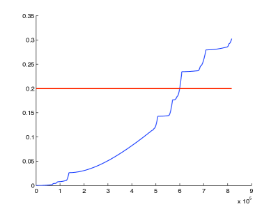
(a) One trajectory

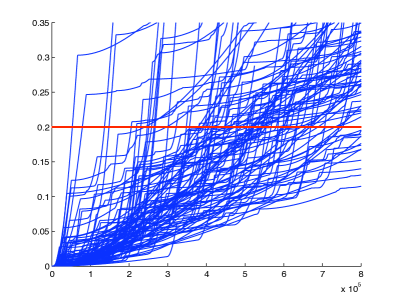
(b) 100 trajectories

Figure 2: Examples of trajectories of thickness loss over time.

Figure 2 shows examples of simulated trajectories of the thickness loss. The slope changes correspond to changes of environment. The observed dispersion is characteristic of the random nature of the phenomenon. Note that the various physical parameters were given by Astrium and will not be discussed here.

The missile is inspected and the thickness loss of the structure under study is measured at each change of environment. Note that the structure is small enough for only one measurement point to be significant. The structure is considered unusable if the loss of thickness reaches $0.2$mm. The optimal maintenance time must therefore occur before reaching this critical threshold, which could cause the collapse of the structure, but not too soon which would be unnecessarily expensive. It should also only use the available measurements of the thickness loss.

III Optimal stopping problem

We now briefly formulate the general mathematical problem of optimal stopping corresponding to our maintenance problem. Let $z=(k_{0},y_{0})$ be the starting point of the PDMP $(X_{t})$. Let $\mathcal{M}_{N}$ be the set of all stopping times $T$ for the natural filtration of the PDMP ($X_{t}$) satisfying $T\leq T_{N}$ that is to say that the intervention takes place before the $N$th jump of process. The $N$th jump represents the horizon of our maintenance problem, that is to say that we impose to intervene no later than $N$th change of environment. The choice of $N$ is discussed below. Let $g$ be the cost function to optimize. Here, $g$ is a reward function that we want to maximize. The optimization problem to solve is the following

$$v(z)=\sup_{\tau\in M_{N}}E_{z}\left[g(X_{\tau})\right].$$

The function $v$ is called the value function of the problem and represents the maximum performance that can be achieved. Solving the optimal stopping problem is firstly to calculate the value function, and secondly to find a stopping time $\tau$ that achieves this maximum. This stopping time is important from the application point of view since it corresponds to the optimum time for maintenance. In general, such an optimal stopping time does not exist. We then define $\epsilon$-optimal stopping times as achieving optimal value minus $\epsilon$, i.e. $v(z)-\epsilon$.

Under fairly weak regularity conditions, Gugerli has shown in [7] that the value function $v$ can be calculated iteratively as follows. Let $v_{N}=g$ be the reward function, and we iterate an operator $L$ backwards. The function $v_{0}$ thus obtained is equal to the value function $v$.

$$\left\{\begin{array}[]{lcl}v_{N}&=&g,\\ v_{k}&=&L(v_{k+1},g),\quad 0\leq k\leq N-1.\end{array}\right.$$

The operator $L$ is a complex operator which involves a continuous maximization, conditional expectations and indicator functions, even if the cost function $g$ is very regular.

$$\begin{array}[]{rl}\displaystyle L(w,g)(z)\equiv&\displaystyle\sup_{u\leq t^{\ast}(z)}\left\{\displaystyle E\left[w(Z_{1})1_{S_{1}<u\wedge t^{\ast}(z)}+g(\Phi(z,u))1_{S_{1}\geq u\wedge t^{\ast}(z)}|Z_{0}=z\right]\right\}\\ &\vee E\left[w(Z_{1})|Z_{0}=z\right].\end{array}$$ (2)

However, we can see that this operator depends only on the discrete time Markov chain $(Z_{n},S_{n})$. Gugerli also proposes an iterative construction of $\epsilon$-optimal stopping times, which is a bit too tedious and technical to be described here, see [7] for details.

For our example of metallic structure, we choose an arbitrary reward function that depends only on the loss of thickness, since this is the critical factor to monitor. Note that we could take into account the other components of our process without any additional difficulty. The reward function is built to reflect the fact that beyond a loss of thickness of 0.2mm, the structure is unusable, so it is too late to perform maintenance. Conversely, if the thickness loss is small, such a maintenance is unnecessarily costly. We use a piecewise affine function $g$ which values are given at the points in the table in Figure 3.

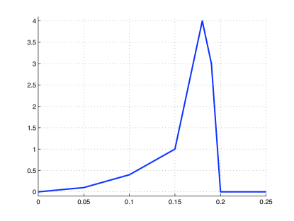
Figure 3: Graphical representation and definition of the cost function as a function of the thickness loss

As for the choice of the computational horizon $N$, numerical simulations show that over 25 changes of environment, all trajectories exceed the critical threshold of $0.2$mm. We will therefore set the time horizon to be the 25th jump ($N=25$).

IV Numerical procedure

It is natural to propose an iterative algorithm to calculate an approximation of the value function based on a discretization of the operator $L$ defined in equation (2). This poses several problems, related to maximizing continuous functions, the presence of the indicator and the presence of conditional expectations. We nevertheless managed to overcome these three problems, using the specific properties of PDMP’s, and in particular the fact that the operator $L$ depends only on the Markov chain $(Z_{n},S_{n})$. Our algorithm for calculating the value function is divided into three stages described below: a quantization of the Markov chain $(Z_{n},S_{n})$, a path-adapted time discretization between jumps, and finally a recursive computation of the value function $v$. Then, the calculation of quasi-optimal stopping time only uses comparisons of quantities already calculated in the approximation of the value function, which makes this technique particularly attractive, see [4] for more mathematical details.

IV-A Quantization

The goal of the quantization step is to replace the continuous state space Markov chain $(Z_{n},S_{n})$ by a discrete state space chain $(\hat{Z}_{n},\hat{S}_{n})$. The quantization algorithm is described in details in e.g. [8] [9] [10] or [11]. The principle is to obtain a finite grid adapted to the distribution of the random variable, rather than building an arbitrary regular grid. We discretize random variables rather than the state space, the idea is to put more points in the areas oh high density of the random variable. The quantization algorithm is based on Monte Carlo simulations combined with a stochastic gradient method. It provides $N+1$ grids $\Gamma_{n},~{}0\leq n\leq N$ of dimension $d+2$, one for each couple $(Z_{n},S_{n})$, with $K$ points in each grid. The algorithm also provide weights for the grid points and probability transition between two points of two consecutive grids.

We note $p_{n}$ the projection to the nearest neighbor (for the Euclidean norm) from $\mathbb{R}^{d+2}$ onto $\Gamma_{n}$. The approximation of the Markov chain $(Z_{n},S_{n})$ is constructed as follows:

$$(\hat{Z}_{n},\hat{S}_{n})=p_{n}(Z_{n},S_{n}).$$

Note that $\hat{Z}_{n}$ and $\hat{S}_{n}$ depend on both $Z_{n}$ and $S_{n}$. The quantization theory ensures that the $L^{2}$ norm of the distance between $(\hat{Z}_{n},\hat{S}_{n})$ and $(Z_{n},S_{n})$ tends to 0 as the number of points $K$ in the quantization grids tends to infinity, see [10].

It should be noted that when the dimension of $Z$ is large, $N$ is large and we want to obtain grids with a large number $K$ of points, the quantization algorithm can be time-consuming. However, we can make this grids calculation in advance and store them. They depend only on the distribution of the process, and not on the cost function. Figure 4 gives an example of quantization grid for the standard normal distribution in two dimensions. It illustrates that the quantization algorithm puts more points in areas of high density.

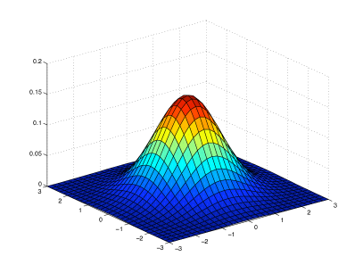
(a) Standard normal density in 2D

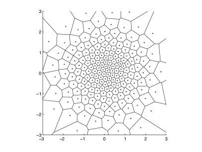
(b) Quantization grid

Figure 4: Example of quantization grid for a normal distribution

IV-B Time discretization

We now wish to replace the continuous maximization of the operator $L$ by a finite maximization, that is to say that we must discretize the time intervals $[0,t^{\ast}(z)]$ for each $z$ in the quantization grids. For this, we choose a time step $\Delta<t^{\ast}(z)$ (which may depend on $z$) and we construct the grids $G(z)=\{t_{1},\cdots,t_{n(z)}\}$ defined by

• $n(z)$ is the integer part minus 1 of $t^{\ast}(z)/\Delta$,

• for $1\leq i\leq n(z)$, $t_{i}=i\Delta$.

We obtain grids that not only do not contain $t^{\ast}(z)$, but in addition, their maximum is strictly less than $t^{\ast}(z)-\Delta$, which is a crucial property to derive error bounds for our algorithm, see [4]. Note also that we only need a finite number of grids $G(z)$, corresponding to the $z$ in the quantization grids $(\Gamma_{n})\,0\leq n\leq N$. Calculation of this time grids can still be made in advance. Another solution is to store only $\Delta$ and $n(z)$ which are sufficient to reconstruct the grids.

In practice, we choose a $\Delta$ that does not depend on $z$. To ensure that we have no empty grid, we first calculate the minimum of $t^{\ast}(z)$ on all grids of quantization, then we choose a $\Delta$ adapted to this value.

IV-C Approximate calculation of the value function

We now have all the tools to provide an approximation of the operator $L$. For each $1\leq n\leq N$, and for all $z$ in the quantization grid at time $n-1$, we set

$$\hat{L}_{n}(w,g)(z) \equiv \max_{u\leq G(z)}\Big{\{}E\Big{[}w(\hat{Z}_{n-1})1_{\hat{S}_{n}<u\wedge t^{\ast}(z)}+g(\Phi(\hat{Z}_{n-1},u))1_{\hat{S}_{n}\geq u\wedge t^{\ast}(z)}|\hat{Z}_{n-1}=z\Big{]}\Big{\}}$$

$$\qquad\vee E\left[w(\hat{Z}_{n})|\hat{Z}_{n-1}=z\right].$$

Note that because we have different quantized approximations at each time step, we also have different discretizations of operator $L$ at each time step. We then construct an approximation of the value function by backward iterations of the $\hat{L}_{n}$:

$$\left\{\begin{array}[]{lcl}\hat{v}_{N}&=&g,\\ \hat{v}_{n-1}(\hat{Z}_{n-1})&=&\hat{L}_{n}(\hat{v}_{n},g)(\hat{Z}_{n-1}),\quad 1\leq n\leq N.\end{array}\right.$$

Then we take $\hat{v}_{0}(\hat{Z}_{0})=\hat{v}_{0}(z)$ as an approximation of the value function $v$ at the starting point $z$ of the PDMP. It should be noted that the conditional expectations taken with respect to a process with discrete state space are actually finite weighted sums.

Theorem IV.1

Under assumptions of Lipschitz regularity of the cost function $g$ and local characteristics $(\Phi,\lambda,Q)$ of the PDMP, the approximation error in the calculation of the value function is

$$||\hat{v}_{0}(z)-v_{0}(z)||_{2}\leq C\sqrt{EQ}$$

where $C$ is an explicit constant which depends on the cost function and local characteristics of the PDMP, and $EQ$ is the quantization error.

Since the quantization error tends to 0 when the number of points in the quantization grid increases, this result shows the convergence of our procedure. Here, the order of magnitude as the square root of the quantization error is due to the presence of indicator functions, which slow convergence because of their irregularity. To get around the fact that these functions are not continuous, we use the fact that the sets where they are actually discontinuous are of very low probability. The precise statement of this theorem and its proof can be found in [4].

IV-D Calculation of a quasi-optimal stopping time

We have also implemented a method to compute an $\epsilon$-optimal stopping time. The discretization is much more complicated and subtle than that of operator $L$, because we need both to use the true Markov chain $(Z_{n},S_{n})$ and its quantized version $(\hat{Z}_{n},\hat{S}_{n})$. The principle is as follows:

• At time $0$, with the values $Z_{0}=z$ and $S_{0}=0$, we calculate a first date $R_{1}$ which depends on $Z_{0}$, $S_{0}$ and on the value that has realized the maximum in the calculation of $\hat{L}_{1}(\hat{v}_{1},g)$.

• We then allow the process to run normally until the time $R_{1}\wedge T_{1}$, that is the minimum between this computed time $R_{1}$ and the first change of environment. If $R_{1}$ comes first, it is the date of near-optimal maintenance, if $T_{1}$ comes first, we reset the calculation.

• At time $T_{1}$, with the values of $Z_{1}$ and $S_{1}$, we calculate the second date $R_{2}$ which depends on $Z_{1}$ and $S_{1}$ and on the the value that has realized the maximum in the calculation of $\hat{L}_{2}(\hat{v}_{2},g)$.

• We then allow the process to run normally until the time $(T_{1}+R_{2})\wedge T_{2}$, that is the minimum between the computed remaining time $R_{2}$ and the next change of environment. If $T_{1}+R_{2}$ comes first, it is the date of near-optimal maintenance, if $T_{2}$ comes first, we reset the calculation, and so on until the $N$th jump time where maintenance will be performed if it has not occurred before.

We have also proved the quality of this approximation by comparing the expectation of the cost function of the process stopped by the above strategy to the true value function. This result, its proof and the precise construction of our stopping time procedure can be found in [4].

This stopping strategy is interesting for several reasons. First, this is a real stopping time for the original PDMP which is a very strong result. Second, it requires no additional computation compared to those made to approximate the value function. This procedure can be easily performed in real time, and only requires an observation of the process at the times of change of environment, which is exactly the available inspection data for our metallic structure. Moreover, even if the original problem is an optimization on average, this stopping rule is path-wise and is updated when new data arrive on the history of the process at each change of environment. Finally, as our stopping procedure is of the form intervene at such date if no change of environment has occurred in the meantime, it allows in some measure to have maintenance scheduled in advance, In particular, our procedure ensures that there will be no need to perform maintenance before a given date, which is crucial for our example as a submarine in operation should not be stopped at short notice.

V Numerical results

We have implemented this procedure for the optimization of the maintenance of the metallic structure described in section II. With our choice of reward function, it is easy to see that the true value function at $z=0$ is 4, which is the maximum of the reward function $g$, and an optimal stopping time is the first moment when the loss reaches 0.18 mm thick (value where $g$ reaches its maximum). This is because the cost function only depends on the thickness loss, which evolves continuously increasingly over time. However, our numerical procedure is valid for any sufficiently regular reward function, and we shall not use the knowledge of the true value function or optimal stopping time in our numerical procedure. Besides, we recall that the thickness loss is not measured continuously.

While running the algorithm described in the previous section, e encountered an unexpected difficulty for the construction of the quantization grids. Indeed, the scales of the different variables of the problem are radically different: from about $10^{-6}$ for $\rho$ to $10^{5}$ for the average time spent in environment 2. This poses a problem in the classical quantization algorithm as searching the nearest neighbor and gradient calculations are done in Euclidean norm, regardless of the magnitudes of the components.

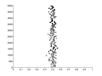
(a) Classical algorithm

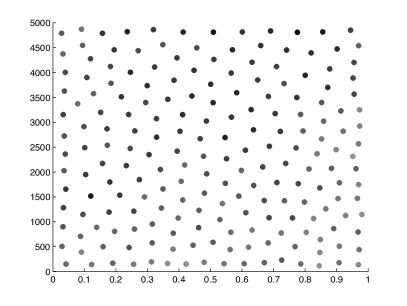
(b) Algorithm with weighted Euclidean norm

Figure 5: Quantization grids for a uniform distribution on $[0,1]\times[0,5000]$

Figure 5 illustrates this problem by presenting two examples of quantization grids for a uniform distribution on $[0,1]\times[0,5000]$. The left image shows the result obtained by the conventional algorithm, the right one is obtained by weighting the Euclidean norm to renormalize each variable on the same scale. It is clear from this example that the conventional method is not satisfactory, because the grid obtained is far from uniform. This defect is corrected by a renormalization of the variables. We therefore used a weighted Euclidean norm to quantify the Markov chain associated with our degradation process.

Figure 6

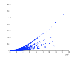
(a) Environment 2, time $T_{1}$

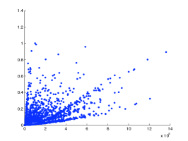
(b) Environment 3, time $T_{2}$

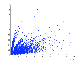
(c) Environment 2, time $T_{10}$

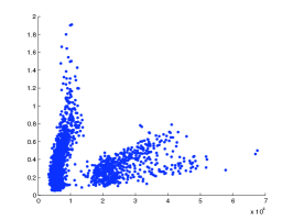
(d) Environment 1, time $T_{15}$

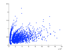
(e) Environment 2, time $T_{19}$

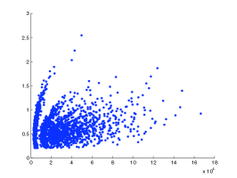
(f) Environment 2,time $T_{25}$

Figure 6: Quantization grids with 2000 points for the inter-jump time (abscissa) and the thickness loss (ordinate). The scale changes for each graph.

shows some projections of the quantization grids with 2000 points that we obtained. The times are chosen in order to to illustrate the random and irregular nature of the grids, they are custom built to best approach the distribution of the degradation process.

Figure 7

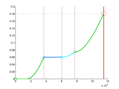
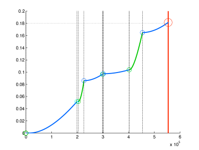
Figure 7: Examples of stopped trajectories with the optimal maintenance time calculated by the algorithm.

shows two examples of computation of the quasi optimal maintenance time on two specific simulated trajectories. The thick vertical line represents the moment provided by the algorithm to perform maintenance. The other vertical lines materialize the moments of change of environment, the horizontal dotted line the theoretical optimum. In both examples, we stop at a value very close to the optimum value. In addition, the intervention did take place before the critical threshold of 0.2mm.

We calculated an approximate value function $v$ in two ways. The first one is the direct method obtained by the algorithm described above. The second one is obtained by Monte Carlo simulation using the quasi-optimal stopping time provided by our procedure. The numerical results we obtained are summarized in Table I.

Number of points	Approximation of the	Approximation of the value
in the quantization	value function by the	function by Monte Carlo with the
grids	direct algorithm	quasi-optimal stopping time
10	2.48	0.94
50	2.70	1.84
100	2.94	2.10
200	3.09	2.63
500	3.39	3.15
1000	3.56	3.43
2000	3.70	3.60
5000	3.82	3.73
8000	3.86	3.75

TABLE I: Numerical results for the calculation of the value function.

We see as expected, that the greater the number of points in the quantization grid, the better our approximation becomes. Furthermore, the specific form of this cost function $g$ indicates that at the threshold of 1, the intervention takes place between 0.15 and 0.2mm, and when the threshold increases, this range is narrowed. We can therefore state that our approximation is good even for low numbers of grid points. The last column of the table also shows the validity of our stopping rule. It should be noted here that this rule does not use the optimal stopping time stop at the first moment when the thickness loss reaches 0.18mm. The method we use is general and implementable even when the optimal stopping time is unknown or does not exist.

Moreover, we can also construct a histogram (Figure 8)

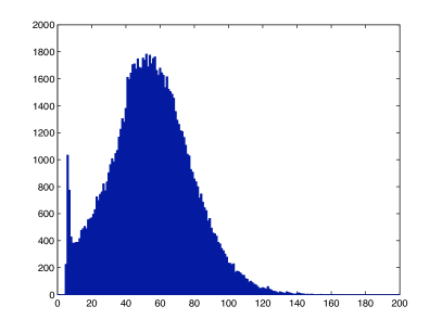
(a) Histogram of 100000 values of the optimal maintenance time expressed in years.

(b) Quantiles.

Figure 8: Distribution and quantiles of the quasi-optimal stopping time.

of the values of our stopping time, that is to say, a histogram of the values of effective moments of maintenance. We can also estimate the probability that this moment is below certain thresholds. These results are interesting for Astrium in the design phase of the structure to optimize margins from the specifications and to consolidate the design margins available. Thus, we can justify that with a given probability no maintenance will be required before the termination date of the contract.

VI Conclusion

We have applied the numerical method described in [4] on a practical industrial example to approximate the value function of the optimal stopping problem and a quasi-optimal stopping time for a piecewise-deterministic Markov process, that is the quasi optimal maintenance date for our structure. The quantization method we propose can sometimes be costly in computing time, but has a very interesting property: it can be calculated off-line. Moreover it depends only on the evolutionary characteristics of the model, and not on the cost function chosen, or the actual trajectory of the specific process we want to monitor. The calculation of the optimal maintenance time is done in real time. This method is especially attractive as its application requires knowledge of the system state only at moments of change of environment and not in continous time. The optimal maintenance time is updated at the moments when the system switches to another environment and has the form intervene at such date if no change of mode takes place in the meantime, which allows to schedule maintenance services in advance.

We have implemented this method on an example of optimization of the maintenance of a metallic structure subject to corrosion, and we obtained very satisfactory results, very close to theoretical values, despite the relatively large size of the problem. These results are interesting for Astrium in the design phase of the structure to maximize margins from the specifications and to consolidate the avaible dimensional margins. Thus, we propose tools to justify that with a given probability that no maintenance will be required before the end of the contract.

The application that we have presented here is an example of maintenance as good as new of the system. The next step will be to allow only partial repair of the system. The problem will then be to find simultaneously the optimal times of maintenance and optimal repair levels. Mathematically, it is an impulse control problem, which complexity exceeds widely that of the optimal stopping. Here again, the problem is solved theoretically for PDMP, but there is no practical numerical method for these processes in the literature. We now work in this direction and we hope to be able to extend the results presented above.

Acknowledgement

This work was partially funded by the ARPEGE program of National Agency for Research (ANR), project FauToCoES, ANR-09-004-SEGI.

References

- [1] T. AVEN and U. JENSEN. Stochastic models in reliability. Spring Verlag, New York, 1999.
- [2] O. L. V. COSTA and M. H. A. DAVIS. Approximations for optimal stopping of piecewise-deterministic process. Math. Control Signals Systems, 1(2):123–146, 1988.
- [3] M.H.A. DAVIS. Markov models and optimization. Chapman and Hall, London, 1993.
- [4] B. DE SAPORTA, F. DUFOUR, and K. GONZALEZ. Numerical method for optimal stopping of piecewise deterministic markov processes. Ann. Appl. Probab., 20(5):1607–1637, 2010.
- [5] J. DEVOOGHT. Dynamic reliability. Advances in nuclear science and technology. Chapman and Hall, Berlin, 1997.
- [6] F. DUFOUR and Y. DUTUIT. Dynamic reliability : A new model. In Proceedings of ESREL 2002 Lambda-Mu 13 Conference, pages 350–353, 2002.
- [7] U.S. GUGERLI. Optimal stopping of a piecewise-deterministic markov process. Stochastics, 19:221–236, 1986.
- [8] G. PAGES. A space quantization methods for numerical integration. J. Comput. Appl. Math., 89(1):1–38, 1998.
- [9] G. PAGES and H. PHAM. Optimal quantization methods for nonlinear filtering with discrete-time observations. Bernouilli, 11(5):892–932, 2005.
- [10] G. PAGES, H. PHAM, and J. PRINTEMS. An optimal markovian quantization algorithm for multidimensional stochastic control problem. Stoch. Dyn., 4(4):501–545, 2004.
- [11] G. PAGES, H. PHAM, and J. PRINTEMS. Optimal quantization methods and applications to numerical problems in finance. In Handbook of computational and numerical methods in finance, pages 253–297, Birkhauser Boston, 2004.