Permissible transitions of the variability classes of GRS 1915+105

Abstract

Context. The Galactic microquasar GRS 1915+105 exhibits at least sixteen types of variability classes. Transitions from one class to another could take place in a matter of hours. In some of the classes, the spectral state transitions (burst-off to burst-on and vice versa) were found to take place in a matter of few to few tens of seconds.

Aims. In the literature, there is no attempt to understand in which order these classes were exhibited. Since the observation was not continuous, the appearances of these classes seem to be in random order. Our goal is to find a natural sequence of these classes and compare with the existing observations. We also wish to present a physical interpretation of the sequence so obtained using two component advective flow model of black hole accretion.

Methods. In the present paper, we compute the ratios of the power-law photons and the black body photons in the spectrum of each class and call these ratios as the ‘Comptonizing efficiency’ (CE). We sequence the classes from the low to the high value of CE. The number of photons were obtained by fitting the spectra of two independent sets of data of each class with disk blackbody and power-law components, after making suitable correction for the absorption in the intervening medium.

Results. We clearly find that each variability class could be characterized by a unique average Comptonizing efficiency. The sequence of the classes based on this parameter seem to be corroborated by a handful of the observed transitions caught by Rossi X-ray timing explorer and the Indian payload Indian X-ray Astronomy Experiment and we believe that future observation of the object would show that the transitions can only take place between consecutive classes in this sequence. Since the power-law photons are produced by inverse Comptonization of the intercepted soft-photons from the Keplerian disk, a change in CE actually corresponds to a change in geometry of the Compton cloud. Thus we claim that the size of the Compton cloud gradually rises from very soft class to the very hard class.

1 Introduction

The enigmatic stellar mass black hole binary GRS 1915+105 (Harlaftis & Greiner, 2004) was first discovered in 1992 by the WATCH detectors (Castro-Tirado et al. 1992) as a transient source with a significant variability in X-ray photon counts (Castro-Tirado et al. 1994). In the RXTE era, GRS 1915+105 was monitored thousands of times in the X-ray band and the scientific results reveal a unique nature of this compact object. The radio observation with VLA suggests apparent superluminal nature of its radio jets. Radio observation constrains that its maximum distance is no more than $13.5$ kpc and that the jet axis makes an angle of $70^{\circ}$ with the line of sight (Mirabel & Rodriguez, 1994).

Continuous X-ray observation of GRS 1915+105 reveals that the X-ray intensity of the source changes peculiarly in a variety of timescales ranging from seconds to days (Greiner et al., 1996, Morgan et al., 1997). Quasi-Periodic Oscillations (QPOs) are observed in a wide range of frequencies. QPOs in this source are associated with different types of X-ray variabilities and their timing properties are correlated with spectral features (Muno et al., 1999, Sobczak et al., 1999, Rodriguez et al., 2002, Vignarca et al., 2003,). The origin of QPO frequencies between $0.5$ to $10$ Hz is identified to be due to the oscillation of the Comptonized photons, presumably emitted from the post-shock region of the low angular momentum (sub-Keplerian) flow (Chakrabarti & Manickam, 2000, hereafter CM00; Rao et al., 2000).

Small scale variabilities of GRS 1915+105 are identified with local variation of the inner disk (Nandi et al., 2000, Chakrabarti & Manickam, 2000; Migliari & Belloni, 2003). Several observers have reported that this object exhibited many types of variability classes (Yadav et al., 1999; Rao, Yadav & Paul, 2000; Belloni et al. 2000, Chakrabarti & Nandi, 2000; Naik et al. 2002a). Depending on the variation of photon counts in different arbitrary energy bands (hardness ratio) and color-color diagram of GRS 1915+105, the X-ray variability of the source was found to have fifteen arbitrarily named ($\alpha,\ \beta,\ \gamma,\ \delta,\ \phi,\ \chi_{1},\chi_{2},\chi_{3},\chi_{4},\ \mu,\ \nu,\ \lambda,\ \kappa,\ \rho,\ \theta$) classes. In a 1999 observation of RXTE, the existence of another class $\omega$ was reported (Klein-Wolt et al., 2002; Naik et al. 2002a). In the so-called $\chi$ (i.e., $\chi_{1}$ to $\chi_{4}$) class, the strong variability as is found in other classes is absent. The classes named $\chi_{1},\chi_{3}$, $\beta$ and $\theta$ are associated with the presence of strong radio jets (Naik & Rao, 2000, Vadawale et al., 2003). To understand the above features from a dynamical point of view, we carried out a correlation study in between temporal and spectral features of this source in different classes. A preliminary report is presented in Pal, Nandi & Chakrabarti (2008, hereafter PNC08).

While a large number of papers have been published in the literature on GRS 1915+105, to our knowledge, there is no work which actually asked the question: are these classes arbitrary, or they appear in a given sequence? The problem lies in the fact that no satellite continuously observed GRS 1915+105. Sporadic observations caught the object in sporadic classes. In the present paper, we try to show that these classes could be parameterized by a common parameter, namely, the ratio between the number of photons in the power-law component and the black body component. We call this as the Comptonizing Efficiency or CE. Since the number of photons in the power-law component depends on the degree of interception by the so-called hot electron cloud or Compton cloud (Sunyaev & Titarchuk, 1980, 1985), different classes are therefore parameterized by the average size of the Compton cloud. Along with the dynamical evolution of CE, we compute the spectrum and the power density spectrum (PDS) for each of the classes. To accomplish the computation of CE, we separate out the photons $\gamma_{BB}$ of the black body component and the photons $\gamma_{PL}$ from the power-law component and take the running ratio CE as a function of time to study how the Compton cloud itself varies in a short time scale. Our findings reveal that the Compton cloud is highly dynamic. We present possible scenarios of what might be occurring to it in different variability classes.

The paper is organized as follows: in the next Section, we present a general discussion of the observation, our criteria of selection of data for analysis and analysis technique. In §3, we discuss the procedure of calculation that is adopted to calculate the photon numbers. In §4, the results are presented. In §5, we present a unifying view where we show that the Comptonizing efficiency may be a key factor to distinguish among various classes. Finally, in §6, we make concluding remarks.

2 Observation & Data Analysis

The RXTE science data is taken from the NASA HEASARC data archive for analysis. We have chosen the data procured in 1996-97 by RXTE as in this period GRS 1915+105 has shown almost all types of variabilities in X-rays. Subsequently, in 1999, another class, namely $\omega$ was seen. In the present paper, since we are interested in sequencing these sixteen classes, we will rename them as follows: I=$\phi$; II=$\delta$; III=$\gamma$; IV=$\omega$; V=$\mu$; VI=$\nu$; VII=$\lambda$; VIII=$\kappa$; IX=$\rho$; X=$\beta$; XI=$\alpha$; XII=$\theta$; XIII=$\chi_{2}$; XIV=$\chi_{4}$; XV=$\chi_{1}$; XVI=$\chi_{3}$). This would be our final sequence also, and hence it is easier to remember. Moreover, theoretical discussions often uses these Greek characters it would be confusing to use these symbols.

During the data analysis we excluded the data collected for elevation angles less than $10^{\circ}$, offset greater than $0.02^{\circ}$ and during the South Atlantic Anomaly (SAA) passage. In Table. 1, the details of the data selection and ObsIDs are given which we analyzed in this paper.

Obs-Id	Class	Date
10408-01-19-00∗	I	29-06-1996
10408-01-09-00	I	29-05-1996
10408-01-18-00∗	II	25-06-1996
20402-01-41-00	II	19-08-1997
20402-01-37-00∗	III	17-07-1997
20402-01-56-00	III	22-11-1997
40703-01-27-00∗	IV	23-08-1999
40403-01-07-00	IV	23-04-1999
10408-01-36-00∗	V	28-09-1996
20402-01-53-01	V	05-11-1997
10408-01-40-00∗	VI	13-10-1996
20402-01-02-02	VI	14-11-1996
20402-01-36-00∗	VII	10-07-1997
10408-01-38-00	VII	07-10-1996
20402-01-35-00∗	VIII	07-07-1997
20402-01-33-00	VIII	18-06-1997
20402-01-31-00∗	IX	03-06-1997
20402-01-03-00	IX	19-11-1996
10408-01-10-00∗	X	26-05-1996
20402-01-44-00	X	31-08-1997
20187-02-01-00∗	XI	07-05-1997
20402-01-30-01	XI	28-05-1997
10408-01-15-00∗	XII	16-06-1996
20402-01-45-02	XII	05-09-1997
20402-01-16-00∗	XIII	22-02-1997
20402-01-05-00	XIII	04-12-1996
20402-01-25-00∗	XIV	19-04-1997
10408-01-33-00	XIV	07-09-1996
10408-01-23-00∗	XV	14-07-1996
10408-01-30-00	XV	18-08-1996
20402-01-50-00∗	XVI	14-10-1997
20402-01-51-00	XVI	22-10-1997

Table 1: The ObsIDs and the dates of RXTE data analyzed in this paper. ^∗ represents the result shown in Fig. 3 of this paper.

Here we discuss how we analyzed the temporal and spectral properties of the data.

2.1 Timing Analysis

In timing analysis of the RXTE/PCA data we use “binned mode” data which was available for 0-35 channels only, with a time resolution of $2^{-7}$ sec and ‘event mode’ data with a time resolution of $2^{-8}$ sec for the rest of the channels. We restrict ourselves in the energy range of $\sim 2-40$ keV for the timing analysis of PCA data. After extracting the light curves (using standard tasks) from the two sets of different modes, we add them by the FTOOLS task “lcmath” to have the whole energy range light curve ($2$ to $40$ keV). The Power Density Spectrum (PDS) is generated by the standard FTOOLS task “powspec” with normalization. Data is re-binned to $0.01$s time resolution to obtain a Nyquist frequency of $50$ Hz as the power beyond this is found to be insignificant. PDSs are normalized to give the squared rms fractional variability per Hertz.

To have the timing evolution of QPO features in different classes, we generate PCA light curves of $2$ to $40$keV photons with $0.01$s time bin. We use the science data accordingly from the ‘binned mode’ and the ‘event mode’ for $10$s time interval in each step. This light curve is then used to make PDS using the ¨powspec¨ task. The dynamic PDS is made by considering the shift of time interval by $1$s. The selection of time interval is done by FTOOLS task ‘timetrans’. The PDSs are plotted accordingly to see the variation of QPO features in a particular class of a few hundred seconds of observation.

2.2 Spectral Analysis

Spectral analysis for the PCA data is done by using “standard2” mode data which have $16$ sec time resolution and we constrained our energy selection up to $40$ keV to match with the timing analysis. The source spectrum is generated using FTOOLS task “SAEXTRCT” with $16$ sec time bin from “standard2” data. The background fits file is generated from the “standard2” fits file by the FTOOLS task “runpcabackest” with the standard FILTER file provided with the package. The background source spectrum is generated using FTOOLS task “SAEXTRCT” with $16$ sec time bin from background fits file. The standard FTOOLS task “pcarsp” is used to generate the response file with appropriate detector information. The spectral analysis and modeling was performed using XSPEC (v.12) astrophysical fitting package. For the model fitting of PCA spectra, we have used a systematic error of $1\%$. The spectra are fitted with diskbb and power law model along with $6.0\times 10^{22}cm^{-2}$ hydrogen column absorption (Muno et al., 1999) and we used the Gaussian for iron line as required for best fitting. During fitting of the spectra we have adopted the method used by Sobczak et al., (1999), to obtain the values of spectral parameters. We have calculated error-bars of 90% confidence level in each case. In case of soft states, the diskbb is found be fitted within $2.5-10.0$ keV. But in case of hard states, the diskbb is fitted within $2.5-5.0$ keV. This upper limit changes dynamically for the fitting of spectra. Table. 2 gives the energy up to which the black body fit is made for each class.

To have the spectral evolution with time for each class, we have generated PCA spectrum ($2.5$ to $40$keV) with a minimum of $16$s time interval along with background spectrum and response matrix. This procedure is repeated with every $16$s shift in time interval since the minimum time resolution in ’standard2’ data is $16$s. We use ‘timetrans’ task to select each and every step of time interval. Spectral evolution (dynamic representation) for a longer duration of observation ($\sim 500$ to $2000$ sec) of each class is plotted to show the local spectral variation in each class.

3 Calculation Procedure

In this section, we discuss the process of calculation of photon numbers using the parameters obtained from spectral fit.

Each spectrum is first fitted within XSPEC environment with the models and constraints mentioned above. The fitting parameters are used to calculate the black body photon counts from the Keplerian component and the power-law photon counts from the Compton cloud. The number of black body photons are obtained from the fitted parameters of the multi-color disk black body model (Makishima et al., 1986). This is given by,

$$f(E)=\frac{8\pi}{3}r_{in}^{2}\cos{i}\int_{T_{out}}^{T_{in}}(T/T_{in})^{-11/3}B(E,T)\,dT/T_{in},$$ (1)

where, $B(E,T)=\frac{E^{3}}{(\exp{E/T}-1)}$ and $r_{in}$ can be calculated from,

$$K=(r_{in}/(D/10kpc))^{2}\cos{i},$$ (2)

where, $K$ is the normalization of the blackbody spectrum obtained after fitting, $r_{in}$ is the inner radius of the accretion disk in km, $T_{in}$ is the temperature at $r_{in}$ in keV. $D$ is the distance of the compact object in kpc and $i$ is the inclination angle of the accretion disk. Here, both the energy and the temperature are in keV. The black body flux, $f(E)$ in counts/s/keV is integrated between $0.1$ keV to the maximum energy (obtained from diskbb model fits with the spectra as done in Sobczak et al., 1999). This gives us with $\gamma_{BB}$, the number of the black body photons in counts/s.

The Comptonized photons $\gamma_{PL}$ that are produced due to inverse-Comptonization of the soft black body photons by ‘hot’ electrons in the Compton cloud are calculated by fitting with the power-law given below,

$$P(E)=N(E)^{-\alpha},$$ (3)

where, $\alpha$ is the power-law index and $N$ is the total counts/s/keV at $1$keV. It is reported in Titarchuk (1994), that the Comptonization spectrum will have a peak at around $3\times T_{in}$. The power law equation is integrated from $3\times T_{in}$ to $40$keV to calculate total number of Comptonized photons in counts/s. The Gaussian function $Ga(E)$ incorporated with power law equation for the presence of line emissions in the spectrum, whenever necessary is given below,

$$Ga(E)=L\frac{1}{\sigma\sqrt{2\pi}}\exp(-0.5\left(E-E_{l})/\sigma)^{2})\right),$$ (4)

where, $E_{l}$ is the energy of emitted line in keV, $\sigma$ is the line width in keV and $L$ is the total number of counts/s in the line. The variation of the Comptonizing Efficiency (CE) with time is plotted to have an idea of how the Compton cloud may be changing its geometry.

We fitted the data with another Comptonization model, namely, the compst (Sunyaev & Titarchuk, 1980). The spectrum is given by,

$$Cst(x) = \frac{\alpha(\alpha+3)}{2\alpha+3}\left(\frac{x}{x_{0}}\right)^{\alpha+3},when\leavevmode\nobreak\ 0\leq x\leq x_{0},$$ (5)

$$= \frac{\alpha(\alpha+3){x_{0}}^{\alpha}}{\Gamma(2\alpha+4)}x^{3}\exp(-x)I(x),when\leavevmode\nobreak\ x\geq x_{0}.\$$

Here $I(x)=\int^{\infty}_{0}t^{\alpha-1}\exp{-t}\left(1+\frac{t}{x}\right)^{\alpha+3},$ $x=E/kT_{e},$ $x_{0}=kT_{in}/kT_{e},$ and $\alpha$ is the spectral index. This $\alpha$ is calculated from $\alpha=\sqrt{\frac{9}{4}+\gamma}-\frac{3}{2}$, where $\gamma=\frac{\pi^{2}m_{e}c^{2}}{3(\tau+\frac{2}{3})^{2}kT_{e}}$. $kT_{e}$ is the electron temperature and $\tau$ is the optical depth of the electron cloud. In the computation, we exclude the hydrogen column absorption feature while calculating CE. This is because we are interested in the photons which were emitted from the disk before suffering any absorption. Thus the variation of CE along with other features (e.g., spectral and QPO frequency variations) will reflect the actual radiative properties of the flow near a black hole.

Figure 1: In the left panel, a sample fitted PCA spectrum along with the diskbb and power law component are shown. The HEXTE data is also added. In the right panel, the same PCA spectrum is fitted with diskbb and compST components.

In Fig. 1, we show an example of the fitted PCA and HEXTE spectrum along with the fitted components. We also show the residuals to characterize the goodness of the fit. In the left panel, the fitting is done with diskbb and power-law components. In the right panel, the same spectrum is fitted with diskbb and compST models. The photon numbers and CE are calculated with the parameters obtained from the fitting. The black body spectrum is simulated with $T_{in}=1.15\leavevmode\nobreak\ ^{+0.057}_{-0.052}$ keV. The calculated number of black body photons from $0.1-6.5$keV is $156.03\leavevmode\nobreak\ ^{+17.10}_{-13.90}$ kcounts/s. In the same way, the power-law spectrum is simulated with the power-law index = $2.057\leavevmode\nobreak\ ^{+0.154}_{-0.147}$. The calculated number of the Comptonized photons between $3.45-40$ keV is $0.39\leavevmode\nobreak\ ^{+0.06}_{-0.05}$ kcounts/s. The ratio between the power-law photon and the black body photon is $0.25\leavevmode\nobreak\ ^{+0.08}_{-0.07}$%. This means that only $0.41$% of the soft photons are Comptonized by the Compton cloud. For the sake of comparison, the simulation with the compST model parameters are found to be $KT_{e}=6.41\leavevmode\nobreak\ ^{+2.55}_{-1.25}$ and $\tau=9.42\leavevmode\nobreak\ ^{+2.88}_{-2.39}$. The number of Comptonized photons within the same range as previous case is $0.41\leavevmode\nobreak\ ^{+0.06}_{-0.05}$ kcounts/s. Thus the ratio between the compST photon and the diskbb photon is $0.26\leavevmode\nobreak\ ^{+0.08}_{-0.07}$%. In Fig. 1a, we also include HEXTE data, and fitted with a power-law. But the spectral fit does not change in slope and the number of photons contributed by HEXTE regime is so low that the basic result of CE is not changed. In Fig. 1b, we give an example where comptST model cannot be fitted with HEXTE data. This is true for many variability classes. We therefore ignore the HEXTE data in the rest of the paper.

In Table. 2, a comparison of the fitted parameters for all the classes is provided with error at $90\%$ confidence level. The first column gives the class name and the second column gives the burst-off (harder) and the burst-on (softer) states, if present, in each class. These states are actually similar to hard and soft states of a black hole, except that the wind plays a major role and thus the states are not all the way hard or soft. The third column gives the black body temperature of the fitted Keplerian disk ($T_{in}$ in keV). The fourth column gives the maximum energy in keV upto which diskbb model is fitted and soft photon number is calculated. The fifth column gives the count rates of the soft photons. The next column gives the index associated with the fitted power-law component. The seventh column gives the derived hard photon counts per second. The eighth column gives the ratio of the photon numbers given in the fifth and the seventh columns. This is the so-called Comptonizing efficiency or CE. We arranged the classes in a way that the average CE changes monotonically. We find it to be high in harder classes such as XIII-XVI and low in the softer classes such as I-II. The final column gives the value of reduced $\chi^{2}$ for the fits. The behavior of average CE will be discussed later.

As mentioned earlier, we fit the spectrum of each class with diskbb and compST model to have the information of $\tau$ and $T_{e}$ of electron distribution inside the Compton cloud. One sample spectrum is taken for each class and fitted with the diskbb and compST model with $n_{H}=6.0\times 10^{22}cm^{-2}$ hydrogen column for absorption and $1\%$ systematic error. The best fitted parameters are given in Table. 3 for comparison with the parameters given in Table. 2. We find that in the cases where both models were used, the CE obtained were very close to each other.

		$T_{in}$	Energy	Soft	Power law	Hard	CE
Class				Photon	index	Photon		$\chi^{2}$
		(keV)	keV	(kcnt/s)		(kcnt/s)	(%)
I	-	$1.67\leavevmode\nobreak\ ^{+0.017}_{-0.017}$	10.2	$275.08\leavevmode\nobreak\ ^{+8.77}_{-8.46}$	$2.927\leavevmode\nobreak\ ^{+0.266}_{-0.255}$	$0.20\leavevmode\nobreak\ ^{+0.04}_{-0.03}$	$0.07\leavevmode\nobreak\ ^{+0.02}_{-0.01}$	1.6
II	-	$1.65\leavevmode\nobreak\ ^{+0.016}_{-0.015}$	10.3	$330.40\leavevmode\nobreak\ ^{+9.48}_{-9.80}$	$2.348\leavevmode\nobreak\ ^{+0.238}_{-0.228}$	$0.16\leavevmode\nobreak\ ^{+0.03}_{-0.02}$	$0.05\leavevmode\nobreak\ ^{+0.01}_{-0.01}$	1.1
III	-	$1.80\leavevmode\nobreak\ ^{+0.015}_{-0.014}$	10.4	$511.13\leavevmode\nobreak\ ^{+12.57}_{-12.22}$	$2.916\leavevmode\nobreak\ ^{+0.352}_{-0.309}$	$0.31\leavevmode\nobreak\ ^{+0.09}_{-0.07}$	$0.06\leavevmode\nobreak\ ^{+0.02}_{-0.01}$	0.60
IV	-	$1.937\leavevmode\nobreak\ ^{+0.025}_{-0.024}$	10.6	$192.21\leavevmode\nobreak\ ^{+7.80}_{-7.41}$	$2.649\leavevmode\nobreak\ ^{+0.308}_{-0.292}$	$0.09\leavevmode\nobreak\ ^{+0.02}_{-0.01}$	$0.05\leavevmode\nobreak\ ^{+0.01}_{-0.01}$	0.98
V	-	$1.421\leavevmode\nobreak\ ^{+0.023}_{-0.022}$	7.0	$468.53\leavevmode\nobreak\ ^{+10.40}_{-10.02}$	$2.330\leavevmode\nobreak\ ^{+0.145}_{-0.140}$	$0.63\leavevmode\nobreak\ ^{+0.085}_{-0.073}$	$0.13\leavevmode\nobreak\ ^{+0.02}_{-0.02}$	1.01
VI	-	$1.752\leavevmode\nobreak\ ^{+0.030}_{-0.029}$	7.0	$370.39\leavevmode\nobreak\ ^{+14.15}_{-13.15}$	$2.578\leavevmode\nobreak\ ^{+0.123}_{-0.119}$	$0.45\leavevmode\nobreak\ ^{+0.04}_{-0.03}$	$0.12\leavevmode\nobreak\ ^{+0.016}_{-0.015}$	1.18
VII	h	$0.933\leavevmode\nobreak\ ^{+0.056}_{-0.049}$	4.5	$229.10\leavevmode\nobreak\ ^{+28.94}_{-22.32}$	$2.106\leavevmode\nobreak\ ^{+0.116}_{-0.112}$	$0.59\leavevmode\nobreak\ ^{+0.07}_{-0.06}$	$0.26\leavevmode\nobreak\ ^{+0.08}_{-0.07}$	0.95
	s	$1.992\leavevmode\nobreak\ ^{+0.022}_{-0.021}$	9.0	$437.22\leavevmode\nobreak\ ^{+11.11}_{-10.62}$	$2.683\leavevmode\nobreak\ ^{+0.219}_{-0.211}$	$0.19\leavevmode\nobreak\ ^{+0.3}_{-0.2}$	$0.04\leavevmode\nobreak\ ^{+0.007}_{-0.006}$	1.2
VIII	h	$1.150\leavevmode\nobreak\ ^{+0.057}_{-0.052}$	6.5	$156.03\leavevmode\nobreak\ ^{+17.10}_{-13.90}$	$2.057\leavevmode\nobreak\ ^{+0.154}_{-0.147}$	$0.39\leavevmode\nobreak\ ^{+0.06}_{-0.05}$	$0.25\leavevmode\nobreak\ ^{+0.08}_{-0.07}$	1.2
	s	$1.900\leavevmode\nobreak\ ^{+0.027}_{-0.026}$	8.0	$432.72\leavevmode\nobreak\ ^{+13.95}_{-13.15}$	$2.983\leavevmode\nobreak\ ^{+0.243}_{-0.234}$	$0.21\leavevmode\nobreak\ ^{+0.03}_{-0.03}$	$0.05\leavevmode\nobreak\ ^{+0.010}_{-0.008}$	1.5
IX	h	$1.382\leavevmode\nobreak\ ^{+0.031}_{-0.029}$	5.75	$382.33\leavevmode\nobreak\ ^{+18.42}_{-16.73}$	$2.505\leavevmode\nobreak\ ^{+0.101}_{-0.099}$	$0.95\leavevmode\nobreak\ ^{+0.09}_{-0.08}$	$0.25\leavevmode\nobreak\ ^{+0.04}_{-0.03}$	1.54
	s	$1.843\leavevmode\nobreak\ ^{+0.022}_{-0.022}$	8.0	$419.92\leavevmode\nobreak\ ^{+11.55}_{-10.97}$	$2.331\leavevmode\nobreak\ ^{+0.160}_{-0.155}$	$0.34\leavevmode\nobreak\ ^{+0.04}_{-0.03}$	$0.08\leavevmode\nobreak\ ^{+0.01}_{-0.01}$	0.99
X	h	$1.042\leavevmode\nobreak\ ^{+0.032}_{-0.030}$	5.25	$320.15\leavevmode\nobreak\ ^{+20.78}_{-18.15}$	$2.142\leavevmode\nobreak\ ^{+0.061}_{-0.060}$	$0.87\leavevmode\nobreak\ ^{+0.05}_{-0.04}$	$0.27\leavevmode\nobreak\ ^{+0.04}_{-0.04}$	1.05
	s	$1.448\leavevmode\nobreak\ ^{+0.023}_{-0.022}$	7.0	$354.87\leavevmode\nobreak\ ^{+12.38}_{-11.58}$	$2.688\leavevmode\nobreak\ ^{+0.176}_{-0.170}$	$0.32\leavevmode\nobreak\ ^{+0.05}_{-0.04}$	$0.14\leavevmode\nobreak\ ^{+0.03}_{-0.02}$	1.5
XI	-	$1.213\leavevmode\nobreak\ ^{+0.082}_{-0.070}$	4.5	$261.36\leavevmode\nobreak\ ^{+38.46}_{-28.74}$	$2.067\leavevmode\nobreak\ ^{+0.062}_{-0.061}$	$0.81\leavevmode\nobreak\ ^{+0.04}_{-0.04}$	$0.31\leavevmode\nobreak\ ^{+0.08}_{-0.07}$	1.01
XII	h	$1.391\leavevmode\nobreak\ ^{+0.039}_{-0.037}$	6.0	$416.84\leavevmode\nobreak\ ^{+25.73}_{-22.85}$	$2.501\leavevmode\nobreak\ ^{+0.089}_{-0.087}$	$1.15\leavevmode\nobreak\ ^{+0.09}_{-0.08}$	$0.28\leavevmode\nobreak\ ^{+0.05}_{-0.04}$	1.3
	s	$1.317\leavevmode\nobreak\ ^{+0.034}_{-0.032}$	5.5	$388.95\leavevmode\nobreak\ ^{+21.46}_{-19.19}$	$3.248\leavevmode\nobreak\ ^{+0.157}_{-0.152}$	$0.65\leavevmode\nobreak\ ^{+0.08}_{-0.07}$	$0.17\leavevmode\nobreak\ ^{+0.03}_{-0.03}$	1.5
XIII	-	$1.200\leavevmode\nobreak\ ^{+0.117}_{-0.094}$	4.5	$126.80\leavevmode\nobreak\ ^{+27.74}_{-18.46}$	$1.968\leavevmode\nobreak\ ^{+0.076}_{-0.074}$	$0.57\leavevmode\nobreak\ ^{+0.03}_{-0.03}$	$0.45\leavevmode\nobreak\ ^{+0.17}_{-0.12}$	1.2
XIV	-	$1.184\leavevmode\nobreak\ ^{+0.113}_{-0.091}$	4.5	$121.04\leavevmode\nobreak\ ^{+25.87}_{-17.37}$	$1.954\leavevmode\nobreak\ ^{+0.081}_{-0.079}$	$0.52\leavevmode\nobreak\ ^{+0.03}_{-0.02}$	$0.43\leavevmode\nobreak\ ^{+0.16}_{-0.12}$	1.0
XV	-	$1.165\leavevmode\nobreak\ ^{+0.053}_{-0.048}$	4.5	$599.39\leavevmode\nobreak\ ^{+58.18}_{-47.51}$	$2.736\leavevmode\nobreak\ ^{+0.057}_{-0.056}$	$4.62\leavevmode\nobreak\ ^{+0.12}_{-0.11}$	$0.77\leavevmode\nobreak\ ^{+0.08}_{-0.07}$	1.3
XVI	-	$1.187\leavevmode\nobreak\ ^{+0.030}_{-0.028}$	5.0	$598.83\leavevmode\nobreak\ ^{+31.99}_{-28.57}$	$2.702\leavevmode\nobreak\ ^{+0.057}_{-0.056}$	$5.30\leavevmode\nobreak\ ^{+0.09}_{-0.09}$	$0.88\leavevmode\nobreak\ ^{+0.10}_{-0.09}$	1.1

Table 2: Parameters for the simulated spectral fits with diskbb plus powerlaw models for all the variability classes.

		$T_{in}$	Energy	Soft	$T_{e}$	$\tau$	Hard	CE
Class				Photon			Photon		$\chi^{2}$
		(keV)	keV	(kcnt/sec)	keV		(kcnt/s)	(%)
I	-	$1.67\leavevmode\nobreak\ ^{+0.017}_{-0.017}$	10.2	$275.08\leavevmode\nobreak\ ^{+8.77}_{-8.46}$	-	-	-	-	-
II	-	$1.65\leavevmode\nobreak\ ^{+0.016}_{-0.015}$	10.3	$330.04\leavevmode\nobreak\ ^{+9.48}_{-9.80}$	-	-	-	-	-
III	-	$1.80\leavevmode\nobreak\ ^{+0.015}_{-0.014}$	10.4	$511.13\leavevmode\nobreak\ ^{+12.57}_{-12.22}$	-	-	-	-	-
IV	-	$1.937\leavevmode\nobreak\ ^{+0.025}_{-0.024}$	10.6	$192.21\leavevmode\nobreak\ ^{+7.80}_{-7.41}$	-	-	-	-	-
V	-	$1.421\leavevmode\nobreak\ ^{+0.023}_{-0.022}$	7.0	$468.53\leavevmode\nobreak\ ^{+10.40}_{-10.02}$	$4.718\leavevmode\nobreak\ ^{+0.983}_{-0.660}$	$14.399\leavevmode\nobreak\ ^{+4.624}_{-4.457}$	$0.61\leavevmode\nobreak\ ^{+0.085}_{-0.073}$	$0.13\leavevmode\nobreak\ ^{+0.02}_{-0.02}$	1.01
VI	-	$1.752\leavevmode\nobreak\ ^{+0.030}_{-0.029}$	7.0	$370.39\leavevmode\nobreak\ ^{+14.15}_{-13.15}$	-	-	-	-	-
VII	h	$0.933\leavevmode\nobreak\ ^{+0.056}_{-0.049}$	4.5	$229.10\leavevmode\nobreak\ ^{+28.94}_{-22.32}$	$4.926\leavevmode\nobreak\ ^{+1.082}_{-0.680}$	$12.432\leavevmode\nobreak\ ^{+2.747}_{-2.246}$	$0.52^{+0.07}_{-0.06}$	$0.22\leavevmode\nobreak\ ^{+0.08}_{-0.07}$	1.5
	s	$1.992\leavevmode\nobreak\ ^{+0.022}_{-0.021}$	9.0	$437.22\leavevmode\nobreak\ ^{+11.11}_{-10.62}$	-	-	-	-	-
VIII	h	$1.150\leavevmode\nobreak\ ^{+0.057}_{-0.052}$	6.5	$156.03\leavevmode\nobreak\ ^{+17.10}_{-13.90}$	$6.410\leavevmode\nobreak\ ^{+2.558}_{-1.255}$	$9.415\leavevmode\nobreak\ ^{+2.879}_{-2.390}$	$0.41\leavevmode\nobreak\ ^{+0.06}_{-0.05}$	$0.26\leavevmode\nobreak\ ^{+0.08}_{-0.07}$	0.90
	s	$1.900\leavevmode\nobreak\ ^{+0.027}_{-0.026}$	8.0	$437.72\leavevmode\nobreak\ ^{+13.95}_{-13.15}$	-	-	-	-	-
IX	h	$1.382\leavevmode\nobreak\ ^{+0.031}_{-0.029}$	5.75	$382.33\leavevmode\nobreak\ ^{+18.42}_{-16.73}$	$3.892\leavevmode\nobreak\ ^{+0.458}_{-0.290}$	$30.926\leavevmode\nobreak\ ^{+4.361}_{-4.360}$	$0.75\leavevmode\nobreak\ ^{+0.09}_{-0.08}$	$0.20\leavevmode\nobreak\ ^{+0.04}_{-0.03}$	1.43
	s	$1.843\leavevmode\nobreak\ ^{+0.022}_{-0.022}$	8.0	$419.92\leavevmode\nobreak\ ^{+11.55}_{-10.97}$	-	-	-	-	-
X	h	$1.042\leavevmode\nobreak\ ^{+0.032}_{-0.030}$	5.25	$320.15\leavevmode\nobreak\ ^{+20.78}_{-18.15}$	$4.612\leavevmode\nobreak\ ^{+0.820}_{-0.563}$	$11.075\leavevmode\nobreak\ ^{+2.876}_{-2.097}$	$0.57\leavevmode\nobreak\ ^{+0.05}_{-0.04}$	$0.18\leavevmode\nobreak\ ^{+0.04}_{-0.04}$	0.92
	s	$1.448\leavevmode\nobreak\ ^{+0.023}_{-0.022}$	7.0	$354.87\leavevmode\nobreak\ ^{+12.38}_{-11.58}$	-	-	-	-	-
XI	-	$1.213\leavevmode\nobreak\ ^{+0.082}_{-0.070}$	4.5	$261.36\leavevmode\nobreak\ ^{+38.46}_{-28.74}$	$5.043\leavevmode\nobreak\ ^{+0.512}_{-0.410}$	$11.906\leavevmode\nobreak\ ^{+1.545}_{-1.321}$	$0.71\leavevmode\nobreak\ ^{+0.04}_{-0.04}$	$0.27\leavevmode\nobreak\ ^{+0.08}_{-0.07}$	1.37
XII	h	$1.391\leavevmode\nobreak\ ^{+0.039}_{-0.037}$	6.0	$416.84\leavevmode\nobreak\ ^{+25.73}_{-22.85}$	$4.131\leavevmode\nobreak\ ^{+0.673}_{-0.472}$	$14.412\leavevmode\nobreak\ ^{+1.486}_{-4.102}$	$0.96\leavevmode\nobreak\ ^{+0.09}_{-0.08}$	$0.43\leavevmode\nobreak\ ^{+0.07}_{-0.07}$	0.98
	s	$1.317\leavevmode\nobreak\ ^{+0.034}_{-0.032}$	5.5	$388.95\leavevmode\nobreak\ ^{+21.46}_{-19.19}$	-	-	-	-	-
XIII	-	$1.200\leavevmode\nobreak\ ^{+0.117}_{-0.094}$	4.5	$126.80\leavevmode\nobreak\ ^{+27.74}_{-18.46}$	$8.918\leavevmode\nobreak\ ^{+1.952}_{-2.305}$	$6.802\leavevmode\nobreak\ ^{+1.935}_{-2.637}$	$0.52^{+0.03}_{-0.03}$	$0.41\leavevmode\nobreak\ ^{+0.17}_{-0.12}$	1.0
XIV	-	$1.184\leavevmode\nobreak\ ^{+0.113}_{-0.091}$	4.5	$121.04\leavevmode\nobreak\ ^{+25.87}_{-17.37}$	$6.616\leavevmode\nobreak\ ^{+2.744}_{-1.227}$	$8.791\leavevmode\nobreak\ ^{+2.221}_{-2.154}$	$0.51\leavevmode\nobreak\ ^{+0.03}_{-0.02}$	$0.42\leavevmode\nobreak\ ^{+0.16}_{-0.12}$	0.88
XV	-	$1.165\leavevmode\nobreak\ ^{+0.053}_{-0.048}$	4.5	$599.39\leavevmode\nobreak\ ^{+58.18}_{-47.51}$	$4.643\leavevmode\nobreak\ ^{+0.823}_{-0.550}$	$8.500\leavevmode\nobreak\ ^{+1.581}_{-1.402}$	$4.10\leavevmode\nobreak\ ^{+0.12}_{-0.11}$	$0.68\leavevmode\nobreak\ ^{+0.08}_{-0.07}$	1.0
XVI	-	$1.187\leavevmode\nobreak\ ^{+0.030}_{-0.028}$	5.0	$598.83\leavevmode\nobreak\ ^{+31.99}_{-28.57}$	$6.616\leavevmode\nobreak\ ^{+2.744}_{-1.227}$	$8.791\leavevmode\nobreak\ ^{+2.221}_{-2.154}$	$5.20\leavevmode\nobreak\ ^{+0.09}_{-0.09}$	$0.87\leavevmode\nobreak\ ^{+0.10}_{-0.09}$	0.88

Table 3: Parameters for the simulated spectral fits with diskbb and comptST model for all the variability classes. Those classes which could not be fitted with this model have been marked with dashes.

4 Results

We discuss below the main results for each class one by one. The Observational IDs are given in Table 1. So far, we have shown that the CE, which were computed model independent way, vary from one variability class to another, i.e., our results did not depend on any specific theoretical model. However, to interpret the results, and to facilitate the discussions, it is instructive to keep a paradigm in mind. In Fig. 2(a-c), we present a cartoon diagram which is basically the two component advective flow (TCAF) model of Chakrabarti & Titarchuk (1995, hereafter CT95), suitably modified to include outflows as in Chakrabarti & Nandi (2000) (Inclusion of the jets and outflows does not make our model a three component model, since the outflows are results of the inflow and formed from the post-shock region, which is the CENtrifugal pressure supported BOundary Layer, or CENBOL.) In the Figure, the BH represents the black hole, the dark shaded disk is the Keplerian flow and the light shaded disk is the sub-Keplerian flow. The CENBOL and the outflow from it intercept the soft photons from the Keplerian disks and may be cooled down if the Keplerian rate is sufficient.

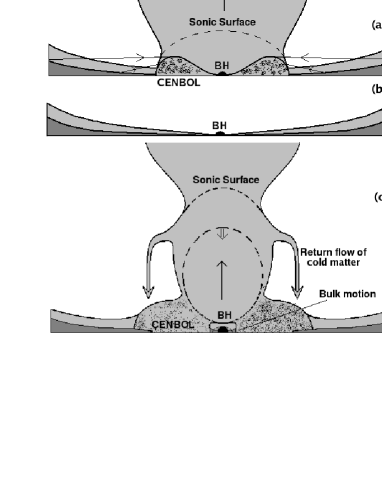
Figure 2: Cartoon diagrams for three major types of variabilities in GRS 1915+105. The classes XIII-XVI belong to the group (a) where the Keplerian rate is low, the CENBOL is large and $<CE>$ is high. Jet/outflow rates may be low and continuous. This is the so-called ‘Hard’ group. The softer classes such as I-IV belong to group (b) where the CENBOL is very small and very little Comptonization may be due to the sub-Keplerian flow only. This is the ‘Soft’ group. The rest of the classes belong to the variations of group (c) or the ‘Intermediate’ group, where, the jet also plays dynamically important role in shaping the spectrum.

In the cartoon diagram of Fig. 2a, the CENBOL is not cooled enough and the Comptonization of the soft photon is done both by the CENBOL as well as the outflow. This configuration typically produces a ‘harder’ state. However, the outflows depends on the shock strength (Chakrabarti, 1999, hereafter C99) and could produce weak jets as in XIII-XIV or strong jets as in XV and XVI (see, Vadawale et al., 2001). In Fig. 2b, the Comptonization is due to the high accretion rate in the Keplerian disk and the CENBOL collapses. As a result, no jets or outflows are formed. This configuration typically produces the soft states. If both the Keplerian and the sub-Keplerian rates are comparable, then the intermediate states would be produced also. In Fig. 2c, we show the situation where the shock strength is intermediate and consequently, the outflow rate is the highest (see, C99; Chakrabarti & Nandi, 2000 and references therein). In this case, there is a possibility that the outflow may be cooled down by Comptonization if the intercepted soft photon flux is high enough and the outflow is temporarily terminated. The flow falls back to the accretion disk, increasing local accretion rate in a very short time scale (seconds). We believe that the variability classes (such as V-XII) some of which show clear softer (burst-on) and harder (burst-off) states alternately and showed evidences of intermittent jets (Klein-Wolt et al. 2002, Rodriguez et al. 2008) belong to this category (Chakrabarti & Manickam, 2000).

We now present the dynamical analysis of the light curves of all the variability classes. While choosing the data duration for a given class, the following considerations have been followed: If the count rate has no obvious rise/fall signatures, we use the data of $500$s. If the count rates have some ‘repetitive’ behavior, we use the data of $500$, $1000$, $1500$s or even $2000$s, which ever is bigger so that at least one full cycle in included in the data chunk. However, in the latter cases, while computing the CE, we use the data from a full cycle only.

In each of Fig. 3(a-p) we show four panels. The top panel is the variation of the photon counts with time. The second panel is the variation of log(power) of the dynamical Power Density Spectra (PDS) which may show presence or absence of quasi-periodic variations or QPOs. The third panel is the dynamic energy spectrum which shows whether the variability class is dominated by hard photons or soft photons. Finally, the bottom panel shows the variation of Comptonizing Efficiency CE calculated using $16$ seconds of binned data. The error bar is provided at $90\%$ confidence level.

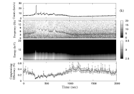
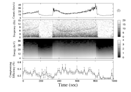
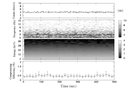
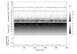
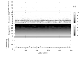
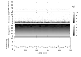
Figure 3: Results of the analysis of (a) I, (b) II, (c) III, (d) IV,(e) V, (f) VI, (g) VII, (h) VIII, (i) IX, (j) X, (k) XI, (l) XII, (m) XIII, (n) XIV, (o) XV, (p) XVI classes are shown. First Panel: Light curve in 2.0-40.0 keV range, Middle Panel: Dynamic PDS of the light curve. Clear evidence of low frequency noise and QPOs are seen. Third panel: Dynamic PCA spectrum showing subtle variations of the spectral characteristics with time. Bottom Panel: Comptonizing Efficiency (CE) in percent, obtained from $16$s binned data.

4.1 Class No. I

The Class I data shows a very short time scale variability with the presence of short scale dips in its light curve. The results are shown in Fig. 3a. Dynamic PDS shows no signature of QPOs and the spectrum is mostly soft in nature. The soft photon number varies at around $330.24$ kcounts/sec while the Comptonized photon number varies around $0.16$ kcounts/sec. The CE is only around $0.05$%. Thus in this class very few black body photons are intercepted by the CENBOL and correspond to a situation similar to that in Fig. 2b.

4.2 Class No. II

In Fig. 3b, we show the result of our analysis of the data that belong to the Class II. In this case, there is an absence of QPO in the dynamic PDS and the spectrum is soft, mostly dominated by the blackbody photons. The CE is around $0.06$%, indicating a situation similar to Class I.

4.3 Class III

The class III data appears to be less variable with a distinct and repeated ’dip’ like features at a time gap of a few seconds. The result is shown in Fig. 3c. The class is a steady soft state with no QPO visible in the PDS. The CE varies around $0.06$% indicating the low interception of the soft photons with the CENBOL.

4.4 Class IV

The results of the analysis of the data of $1000$s in class IV is shown in Fig. 3d. The photon count seems to be steady at around $10000$ counts/sec for most of the time but sometimes for a duration of around $100$ sec the photon count is decreased to about $2000$ counts/sec. In the whole class, no QPO is observed and whenever the photon count is low, the spectrum appears to become harder. The CE remains low at around $0.07$.

The four classes I-IV belong to the softer class. The CE is very low, even when the Keplerian rate is high (spectrum is dominated by soft photons). This means that the CENBOL is very small in size and hence the QPOs are also absent. In our picture, these cases would correspond to that in Fig. 2b, only accretion rates vary. From the count rates, it appears that the disk rates are intermediate in classes I and II while it is high in class III. The sub-Keplerian rate is low in class II, but is intermediate in classes I and III.

4.5 Class V

The result of our analysis for $500$s of data of class V is shown in Fig. 3e. In this class, the spectrum, while remaining soft shows a considerable fluctuation. CE remains low at around $0.05\%$ to $0.15\%$. It goes up when the spectrum is harder. This shows that the Keplerian rate may be changing rapidly and the CENBOL is not really formed, i.e., the sub-Keplerian flow has very low energy and/or angular momentum (C90).

4.6 Class VI

The analysis of $500$s of class VI data is shown in Fig. 3f. The fluctuations of the photon count rate and the spectrum are erratic. QPOs are visible and CE is higher only when the spectrum is harder. CE varies between $0.04$% to $\sim 0.3$%.

4.7 Class VII

The result of our analysis of $1000$ seconds of data of class VII is shown in Fig. 3g. For the first $200-600$ sec the photon number varies between $10000$ and $30000$ counts/sec. The black body photon rate of the simulated spectrum is around $300$ kcounts/sec and Comptonized photon rate is around $0.19$ kcounts/sec. This class is a mixture of the burst-off and burst-on states. When the photon count is higher, the spectrum is softer and the object is in the burst-on state and when the photon count rate is lower, the spectrum is harder and object is in burst-off state. The CE factor varies between $0.05$% to $\sim 0.1$%. Here too, the physics of varying the Comptonizing region (and thus the CE factor) is similar to what is seen in classes VIII-IX below. At the end of the $400$s span when the burst-off state starts, a strong spike in both the CE factor and QPO frequency are observed, indicating a sudden flaring in the CENBOL configuration.

4.8 Class VIII

An analysis of a $500$s chunk of the data of class VIII of observation is shown in Fig. 3h. In the class VIII, the photon counts become high $\sim 30000$/sec and low ($\sim 10000$/sec) aperiodically at an interval of about $50-75$s. In the low count regions, the spectrum is harder and the object is in the burst-off state. Distinct QPOs are present and at the same time, the Comptonizing efficiency is intermediate, being neither as high as in the class no. XIII-XVI, nor as low as in class I-III. In CENBOL picture, low frequency OPOs are indicators of the shock oscillations (CM00). As discussed before, in this case the strength of the shock is intermediate and produces strong outflows (CM00). In the fitted spectrum, the Keplerian photon varies between $150$ to $450$ kcounts/sec and Comptonized photon varies between $0.39$ to $0.21$ kcounts/sec. The CE factor becomes high at $0.25$%. The CENBOL is cooled down. After the matter which fell back on the CENBOL is totally drained, the burst-off state is resurfaced with a lower CE (less than $0.1\%$).

4.9 IX class

The result of our analysis of the class IX data is shown in Fig. 3i. This class contains a cyclic variation of the hard and soft photons with roughly $75$s of periodicity. The blackbody photon count in the simulated spectrum varies between $350$ to $420$ kcounts/s and Comptonized photon counts vary around $0.95$ to $0.34$ kcounts/s. In the harder state (low count regions), the CENBOL is prominent and the Keplerian component is farther away. Thus the QPO is prominent there also. A gradual softening of the hard spectrum indicates that the Keplerian disk is moving towards the black hole and the CENBOL is becoming smaller in size while still retaining its identity. Keplerian photon interaction increases with CENBOL size and CE rises to a maximum of $0.25$%. At the peak of the light curve, the CENBOL, which is also the base of the jet is cooled down due to the increased optical depth.

4.10 Class X

The result of analysis of $1600$s of Class X data is shown in Fig. 3j. In the first phase of $600$ sec, the quasi periodic variation of photon counts takes place in gradually decreasing period from $10000$ counts/sec to $30000$ counts/sec. In this phase, the spectrum is soft and the QPO is seen only when the photon count is low. Here, the CENBOL is visible when the Keplerian flow is going far away from time to time. The CE varies around $0.14\%$.

In next $800$ sec the spectrum is harder and the distinct variation of QPO frequency (from $12$ Hz to $3$ Hz) indicates the variation of the shock location. However, in this phase, CE is varying around $0.27\%$. This means that outflow is taking an active role in intercepting the soft-photons.

4.11 Class XI

Class XI is an intermediate class in which QPO is always observed, the QPO frequency is generally correlated with the count rate (as in XIII-XVI classes discussed below). Since this class displays a long time variation, we analyze the data of $2000$s. Fig. 3k shows the result. The CE varies between $0.05$% to $\sim 0.6$%. The spectrum shows that the Keplerian rate is not changing much, but the sub-Keplerian flow fluctuates, perhaps due to failed attempt to produce sporadic jets. The CE varies considerably and so does the CENBOL.

4.12 Class XII

The result of the analysis of a $1000$s data of class XII is shown in Fig. 3l. This class can be divided in two regions depending on the photon count rates. In the soft dip region the photon count rate is lower than $10000$ counts/sec. In this region, the spectrum is softer and the CE amount of interaction is around $0.17\%$.

In the other (hard dip) region, say between $350$s and $820$s, the photon count is higher and varies from $10000$ counts/sec to $30000$ counts/sec. In this region, CE reaches a high value of $0.28$%. The QPO is also present. Here, the CE factor, which is linked to the geometry of the Comptonizing region, is anti-correlated with the QPO frequency (and correlated with shock location, i.e., CENBOL size). In the third panel, where the dynamic spectrum is drawn, we note that between the soft dip and the hard dip, the low energy photon intensity is not changing much, while the intensity of spectrum at higher energies is higher. This indicates that the sub-Keplerian rate is high in the hard dip state.

4.13 Classes No. XIII & XIV

XIII and XIV classes have low soft X-ray fluxes with less intense radio emissions. Dynamic PDS shows a distinct QPO at around $3$ Hz in class XIII and around $5$ Hz in class XIV. The X-ray photon is significant up to $40$ keV with a flatter power-law slope, which signifies that the source belongs to a hard state. The results are given in Fig. 3m and Fig. 3n. The Comptonizing efficiency in XIII and XIV classes is around $0.4-0.5$%.

4.14 Classes no. XV & XVI

The classes XV and XVI correspond to the radio-loud states, whereas classes XIII and XIV are in radio-quiet states (Vadawale et. al., 2001). In both the cases, the dynamic PDSs show a strong QPO feature around $4$ Hz and $0.8$ Hz respectively throughout the particular observation and the spectrum is dominated by the hard power law. Results are shown in Fig. 3o and Fig. 3p. Around $0.77$% of the soft photons are intercepted by the CENBOL in XIII class, whereas it is $0.88$% in XVI class. In our picture, the CENBOL (Fig. 2a) oscillates to produce the observed QPOs (Chakrabarti, 1997; CM00). Generally, XIII-XVI classes are in harder states and in the language of two component model (CT95, C97), the Keplerian rate is low and unable to cool the CENBOL and jet combined which are produced by the sub-Keplerian flows. Whether the jets would be produced or not depends on the shock strength (C99).

5 Comptonizing efficiency in different classes: an unifying view

In the above sections we have analyzed the data of all the sixteen classes. We presented the light curves, the dynamical energy and power density spectra and the ratio of the power-law photons to the black body photons from the simulated fit of the original spectra. In the literature, there has been so far no discussion on the sequence in which the class transitions should takes place. Also, there is no discussion on which physical properties of the flow, the characteristics of the variability classes depend. In the present paper, we analyzed many aspects of the variability classes which may be understood physically from the two component advective disk paradigm. Since CE behaves differently in various classes, it may play an important role in distinguishing various classes. This CE is directly related to the size and optical depth of the Compton cloud which determines the fraction of the injected soft photon which are intercepted by the Comptonizing region.

Figure 4: Variation of average Comptonizing efficiency ($<CE>$) for different variability classes of GRS 1915+105. The error-bars were calculated from the excursion of CE in a given class. Filled squares and triangles represent $<CE>$ for two sets of variability classes. Generally softer classes have smaller $<CE>$ and harder classes have higher $<CE>$.

Though CE varies very much in a given spectral class, it is instructive to compute the average CE in a given class (averaged over a period characterizing the class). We denote this as $<CE>$. In Fig. 4, we present the variation of log($<CE>$) in various classes. We placed error bars also in all the average values which are at 90% confidence level. We arranged arbitrarily defined sixteen classes in a manner so that $<CE>$s are monotonically increasing. This gives rise to a sequence of the variability class shown in the X-axis. In classes X and XII we did not average CE over both hard and soft regions, since it is believed that the soft regions are produced due to sudden disappearance of the hard region (e.g., Nandi et al. 2001). Thus, while placing them in the plot, we considered the average over the burst-off (harder) state only. To show that the sequence drawn is unique, we plotted the average values of two sets of data of all the classes. The average of the first set is drawn with a dark square sign and the average of the second set is drawn with a dark triangle sign. The individual error bars are drawn with solid and dashed lines respectively. In both the sets, the sequence is identical with softer classes to the left and harder classes to the right. Based on the nature of the variations of CE, we divided these classes into three groups corresponding to three types of accretion shown in Fig. 2(a-c). Classes I to IV belong to ‘softer’ state and classes XIII-XVI belong to ‘harder’ state. The rest of the classes belong to the ‘intermediate’ state.

The above findings of alignment in average CE variation shows that it plays a significant role in distinguishing the variability classes. Moreover, as we discussed already, the variation in CE for a given class is due to the softening and hardening of the spectra in a much shorter time-scale and thus is related to ‘local’ physical processes, such as interaction with winds and outflows, which, in turn, depends on the existence or non-existence of CENBOL, i.e., the spectral states.

Figure 5: Variation of averaged Comptonizing efficiency ($<CE>$) for different variability classes of GRS 1915+105. In the left panel, we show the results for the data set plotted with filled squares in Fig. 4, and the right panel, we show the results of the data plotted with filled triangles in Fig. 4. The averages in hard and soft chunks are placed separately with filled circles. In class X averages of three chunks (burst on, pre-spike and post-spike) are plotted with filled circle, filled box and filled circle respectively. The sequence is found to remain the same in both sets of data. We placed classes X and XII according to $<CE>$ in the hard (pre-spike) region since the softer regions are believed to be produced due to totally different physical processes.

In Fig. 5 (a-b), we plotted the results of these two sets of analysis separately. We show separate averages over CE in the burst-off and burst-on states (as two dark circles) when they are present as well as the global average over CE in a given class by filled squares (except classes X and XII where the physics is different and it is meaningless to talk about the overall average; and hence only average over the harder region is plotted.).

In Chakrabarti et al. (2004) and Chakrabarti et al. (2005), it was mentioned that although many observations were made of GRS 1915+105, only a few cases, direct transitions were observed. In particular, using Indian X-ray Astronomy Experiment (IXAE) they showed direct evidences of $\kappa\rightarrow\rho$ (VIII $\rightarrow$ IX), $\chi\rightarrow\rho$ (XIII $\rightarrow$ IX), $\chi\rightarrow\theta$ (XIII$\rightarrow$ XII) and $\rho\rightarrow\alpha$ (IX$\rightarrow$ XI) transitions in a matter of hours. In Naik et al. (2002), IXAE data was used to argue that $\rho$ class variability could have changed to $\chi$ class via $\alpha$ class (i.e., IX $\rightarrow$ XI $\rightarrow$ XII). In Nandi et al. (2001), it was shown that the $\theta$ class (Class XII) is rare and the observed soft-dip is perhaps due to the disappearance of the inner region by magnetic rubber band effect. Accepting that class XII as anomalous, we find from Fig. 4 that the observed transitions reported in Chakrabarti et al. (2004, 2005) and Naik et al, 2002 are ‘naturally’ explained. For instance, $\chi\rightarrow\rho$ ($\theta$ and $\beta$ being anomalous and intermediate $\alpha$ has been reported by Naik et al. 2002), $\rho\rightarrow\alpha$ ($\beta$ being anomalous) and $\kappa\rightarrow\rho$, are expected from our analysis. Similarly, we can claim that there should not be any transitions such as I $\rightarrow$ IX; III$\rightarrow$ VII; for example. We believe that if we carry out spectro-photometry of GRS 1915+105 continuously (Chakrabarti et al. 2008), then we may be able to catch the transition from one type to another more often and verify if the sequences we mentioned here need further refining.

6 Conclusions

In this paper, we have analyzed all known types of light curves of the enigmatic black hole GRS1915+105 and computed the dynamical nature of the energy and the power density spectra. We did not characterize these classes by conventional means, such as using hardness ratios defined in certain energy range since such a characterization does not improve our view about the physical picture. Furthermore, characterization using certain energy range is possible only in a case by case basis, and is not valid for the black holes of all masses. Instead, we asked ourselves whether we can distinguish one class from another from physical point of view purely in a model independent way. We observed that independent of what the nature of the Compton cloud is, the weighted mean $<CE>$ of Comptonizing efficiency (CE) obtained every 16 seconds of the binned data, increases monotonically as the class varies. This pattern we find was verified with two sets of data covering all the variability classes. So, ¡CE¿ is not arbitrary – it is characteristics of a class. Based on the values of ¡CE¿, it is observed that the classes belong to three states: Classes I-IV in softer states, Classes V-XII in intermediate states, and Classes XIII-XVI belong to the harder state.

When the weighted average value of CE is monotonically arranged, we obtain a sequence which appears to be followed during the actual transitions. Indeed, when comparing with available data of PCU of RXTE and the Indian payload IXAE onboard IRS-P3, the transitions from one class to another as reported in the literature do follow our sequence. Given that a large variation of CE occurs in a given variability class, it is puzzling why the sequence of the classes obtained by us should follow changing the CE values averaged over the whole class. It is possible that a specific value of $<CE>$ actually forces the system to be in a given class, just as a parameter such as wind speed decides the mean angle of an oscillating pendulum. The excursion of CE in that class could be due to totally different physical process and not necessarily due to interception of soft photons by the CENBOL alone. May be the mass-loss rate of CENBOL is playing a role, which in turn depends on the shock strength.

In the two component model of the Chakrabarti-Titarchuk (CT95), the CENBOL and associated outflow play the role of the Compton cloud. In this model, the increase in Compton efficiency can be affected in several ways: (i) by increasing the shock location increases the size of the CENBOL which intercepts larger number of soft photons and/or (ii) by increasing the accretion rate of the sub-Keplerian component, which increases the optical depth and scatter more soft photons to produce power-law photons. In CT95 and C97 it was shown that harder states are produced by both the effects mentioned above. Indeed, we find that the classes with harder states have more CE. Shifting of the shock locations is possible by changes in viscosity or changes in cooling rate in the post-shock region. The time scales of such effects in a sub-Keplerian flow could take hours. Time scale of changing the global sub-Keplerian flow rates could be comparable to the free-fall time from the outer edge, i.e., of the order of a day or so. On the other hand, in Classes VII and VIII etc., the CE changes in a matter of minutes. Such a short time variability of Comptonizing efficiency is possible if the base of the outflow is abruptly cooled and returned back to the disk increasing the accretion rate of the Keplerian/sub-Keplerian rates locally (CM00).

In this paper, we find that the $<CE>$ is really important in deciding the sequence. However, for a given class, the degree of excursion of CE in a given variability type must depend on another parameter, such as the outflow rate which in turn depends on the shock strength. A simple estimate (C99) suggests that the shock strength decides the outflow rate and hence the time taken by the base of the outflow to reach unit optical depth $\tau$ for Compton scattering (CM00). For a very strong shock, this outflow rate is very weak, as is evidenced by weak (few tens of miliJansky) radio flux even for ‘radio-loud’ classes. For intermediate shock strength the outflow rate is higher, and it is easier to have $\tau=1$ in a short time scale (CM00) and fractional change in CE also becomes high. In classes XII-XVI, we not only see CE to be very high, the fractional change in CE is very small as well. The aspect of classification in terms of outflow rate is being looked into. The analysis is in progress and will be reported elsewhere.

- (1) Belloni, T., Klein-Wolt, M., Mendez, M., van der Klis, M. & van Paradijs, J., 2000, A&A 355, 271
- (2) Castro-Tirado, A. J., Brandt, S. & Lund, S., 1992, IAU Circ 5590
- (3) Castro-Tirado, A. J. et. al. 1994, ApJS 92, 469
- (4) Chakrabarti, S. K. 1990, Theory of Transonic Astrophysical Flows, World Scientific Co.
- (5) Chakrabarti, S. K. 1997, ApJ 484, 313
- (6) Chakrabarti, S. K. 1999, A&A 351, 185 (C99)
- (7) Chakrabarti, S.K. & Manickam, S.G. 2000, ApJ, 531, L41 (CM00)
- (8) Chakrabarti, S. K. & Nandi, A. 2000, IJP, 75B(1), 1
- (9) Chakrabarti, S. K., Nandi, A., Manickam, S. G., Mandal, S., 2002, A & A, 579, L21
- (10) Chakrabarti, S. K., Nandi, A., Chatterjee, A. K., Choudhury, A. K. & Chatterjee, U., 2005, A&A, 431, 825
- (11) Chakrabarti, S. K., Nandi, A., Choudhury, A. & Chatterjee, U., 2004, ApJ, 607, 406
- (12) Chakrabarti, S. K. & Titarchuk, L. G., 1995, ApJ 455, 623 (CT95)
- (13) Chakrabarti, S.K. et al. 2008, in Observational Evidence for Black Holes in the Universe, (Ed.) S.K. Chakrabarti, 409 (AIP: NY)
- (14) Greiner, J., Morgan, E. H. & Remillard, R. A., 1996, ApJ, 473, 107
- (15) Harlaftis, E. T. & Greiner, J., 2004, A&A, 414, L13
- (16) Klein-Wolt, M., et. al. 2002, MNRAS 331, 745
- (17) Makishima, K. et. al. 1986, ApJ 308, 635
- (18) Migliari, S. & Belloni, T. 2003, A&A 404, 283
- (19) Mirabel, I. F., Rodriguez, L. F. 1994, Nat 371, 46
- (20) Morgan, E. H., Remillard, R. A. & Greiner, J. 1997, ApJ 482, 993
- (21) Morrison, R., McCammon, D. 1983, ApJ 270, 119
- (22) Muno M. P., Morgan, E. H. & Remillard, R. A., 1999, ApJ 527, 321
- (23) Naik, S. & Rao, A. R. 2000, A&A 362, 691
- (24) Naik, S., Rao, A. R., & Chakrabarti, S. K., 2002a, JApA 23, 213
- (25) Naik, S., Agrawal, P.C., Rao, A.R. & Paul, B., 2002b, MNRAS 330, 487
- (26) Nandi, A., Manickam, S. G. & Chakrabarti, S. K., 2000, IJP 74B, 331
- (27) Nandi, A., Chakrabarti, S.K., Vadawale, S.V. & Rao, A.R., 2001, A&A 380, 245
- (28) Nandi, A., Manickam, S. G. & Chakrabarti, S. K., 2001, MNRAS 324, 267
- (29) Pal, P. S., Nandi, A. & Chakrabarti, S. K. 2008, AIPC 1053, 209
- (30) Rao, A.R., Yadav, J.S., and B. Paul, 2000, ApJ, 544, 443
- (31) Rao, A. R., Naik, S., Vadawale, S. V. & Chakrabarti, S.K., 2000, A&A 360, 25
- (32) Rodriguez, J., Durouchoux, Ph. & Mirabel, I. F., et al., 2002, A&A 386, 271
- (33) Rodriguez, J., Shaw, S. E. & Hannikainen, D. C., et al., 2008, ApJ 675, 1449
- (34) Shakura, N. I. & Sunyaev, R. A. 1973, A&A 24, 337
- (35) Sobczak, G. J., Mclintock, J. E., Remilard R. A. et al. 1999, ApJ 520, 776
- (36) Sunyaev, R. A. & Titarchuk, L. G., 1980, ApJ 86, 121
- (37) Titarchuk, L, 1994, ApJ 434, 313
- (38) Vadawale, S. V., Rao, A. R. & Chakrabarti, S. K. 2001, A&A 372, 793
- (39) Vadawale, S. V., Rao, A. R. & Nandi, A., & Chakrabarti, S.K., 2001, A&A 370, L17
- (40) Vadawale, S. V., Rao, A. R. & Naik, S., et al., 2003, ApJ 597, 1023
- (41) Vignarca, F., Migliari, S. & Belloni, T., et al., 2003, A&A 397, 729
- (42) Yadav, J.S. et al., 1999, ApJ, 517, 935