Modeling the dynamics of biomarkers during primary HIV infection taking into accountthe uncertainty of infection date

Abstract

During primary HIV infection, the kinetics of plasma virus concentrations and CD4$+$ cell counts is very complex. Parametric and nonparametric models have been suggested for fitting repeated measurements of these markers. Alternatively, mechanistic approaches based on ordinary differential equations have also been proposed. These latter models are constructed according to biological knowledge and take into account the complex nonlinear interactions between viruses and cells. However, estimating the parameters of these models is difficult. A main difficulty in the context of primary HIV infection is that the date of infection is generally unknown. For some patients, the date of last negative HIV test is available in addition to the date of first positive HIV test (seroconverters). In this paper we propose a likelihood-based method for estimating the parameters of dynamical models using a population approach and taking into account the uncertainty of the infection date. We applied this method to a sample of 761 HIV-infected patients from the Concerted Action on SeroConversion to AIDS and Death in Europe (CASCADE).

, , and

t1Received a Ph.D. grant from CASCADE Concerted Action on SeroConversion to AIDS and Death in Europe (European Commission Framework Program 6). t2On behalf of the CASCADE Collaboration.

1 Introduction

Primary Human Immunodeficiency Virus (HIV) infection is a crucial period during HIV infection history where there is a viral burst due to the spread of the virus through target cells, mainly CD4$+$ T lymphocytes (CD4). The dynamics of markers at that time is believed to partly determine the evolution of the infection in the future [(Mellors et al., 1995)]. For instance, the peak of viral load has been shown to be predictive of the viral setpoint, that is, the plasma HIV RNA level at which patients often stay for several years [(Lindback et al., 2000)] unless they are treated. This viral setpoint is associated with clinical progression [(Mellors et al., 1995)].

Parametric and nonparametric descriptive models have been suggested for fitting repeated measurements of CD4 and HIV RNA (or viral load) [(Dubin et al., 1994); (Desquilbet et al., 2004); (Pantazis et al., 2005); (Hecht et al., 2006); (Geskus et al., 2007)]. A mechanistic approach based on ordinary differential equations (ODE) has also been suggested [(Phillips, 1996); (De Boer and Perelson, 1998)]. These mathematical models present several advantages. First, they are based on biological knowledge. Therefore, the parameters may have direct biological meaning and the relationship between markers is modeled through biological mechanisms rather than parametric correlation structures. Second, this type of dynamical model is able to capture complex interaction between markers. For instance, these models can predict the decrease of viral load following the peak as a consequence of the limitation of target cells. The first models used in this context gave important insights on the dynamics of the infection and how to control it [(Nowak et al., 1997b); (Little et al., 1999)]. Numerous attempts to improve models have been published [(De Boer and Perelson, 1998); (Wick, 1999); (Stafford et al., 2000)]. Most often, the parameters of these models are not estimated and values which appear “reasonable” are chosen [(Phillips, 1996)]. Indeed, estimating the parameters in such models is difficult. To improve identifiability, random effects models (or population approach) can be used. However, the combination of nonlinear ODE systems and random effects leads to difficult numerical problems [(Putter et al., 2002); (Filter, Xia and Gray, 2005); (Huang, Liu and Wu, 2006); (Samson, Lavielle and Mentré, 2006); (Guedj, Thiébaut and Commenges, 2007a); (Cao, Fussmann and Ramsay, 2008)]: for maximizing the likelihood we need to compute multiple integrals with a dimension equal to the number of random effects included in the model and to solve numerically the ODE system; all steps ask for intensive computations.

The dynamics of the biomarkers during primary HIV infection is quite complex. In the few studies where ODE models have been used in the context of primary infection, the parameters were estimated from the viral load data only [(Kaufmann et al., 1998); (Little et al., 1999); (Stafford et al., 2000); (Lindback et al., 2000); (Ciupe et al., 2006); (Ribeiro et al., 2010)] or the individual fit of the CD4 counts data was very bad [(Murray et al., 1998)]. Moreover, these works did not use random effects models.

In the primary HIV infection context, the system is in a “trivial” equilibrium state without virus and it is disrupted by the introduction of a small quantity of viruses (the “infection event”). The date of infection must thus be known (in contrast to studies of the response to a treatment initiation far from the infection) if we want to compute the trajectories of markers. However, this date is most often unknown. Generally, the only available information is the date of the last seronegative test and first seropositive test or first detectable HIV RNA load. In some cohort studies (such as the Multicenter AIDS Cohort study [(Munoz et al., 1992)]) the last seronegative date is prospectively identified during follow-up. In most cases, patients are seropositive at entry into the cohort and the last seronegative date is retrospectively recorded. Usually, the date of seroconversion is imputed at the midpoint between last negative and first positive HIV serology test [(Fidler et al., 2007)]. Several methods have been suggested for estimating this date according to the marker values [(Berman, 1990); (DeGruttola, Lange and Dafni, 1991); (Dubin et al., 1994); (Geskus, 2000)]. (Geskus et al., 2007) performed a conditional mean imputation to estimate the date of infection that was used as the baseline for linear mixed models.

In the present paper we propose a method for estimating the parameters of dynamic models using a population approach taking into account the uncertainty of the infection date. We estimate the parameters of a dynamical model using HIV RNA and CD4 count data in a large collaboration including cohorts of patients with a documented date of negative and positive HIV serologies (HIV seroconverters).

There are several direct applications of such an approach. First, we can estimate fundamental parameters such as virion clearance, the infected cell death rate [(Perelson et al., 1997)], virus infectivity [(Wilson et al., 2007)] which determines the rate at which T-cells are infected for given virus concentration, or the basic reproduction number $R_{0}$ [(Anderson and May, 1991)] which is defined as the average number of secondary infections that would be caused by the introduction of a single infected cell into an entirely susceptible population of cells; this number reflects the ability of the infection to spread and to persist in the organism. Second, the huge variability in the peak level of HIV RNA and of the viral setpoint in the population [(Kaufmann et al., 1998); (Little et al., 1999)] can be explained by the variability of parameters that carry a direct biological interpretation (cell death rates, virus infectivity, virus production$,\ldots$). Third, the effect of patient characteristics or interventions could be assessed through their biological mechanism. For instance, one could look at the effect of an antiretroviral regimen combining reverse transcriptase inhibitors (blocking the infection of new cells) and protease inhibitors (generating a higher proportion of noninfectious virion) [(Wu and Ding, 1999)] for defining the optimal time of treatment initiation for each patient. It would also be interesting to look at the effect of the transmission of mutated viruses [(Fidler et al., 2006)] or host genetics characteristics [(Fellay et al., 2007)] on the early dynamics. Furthermore, the probability distribution of the date of infection could be useful at the population level for defining the incidence of HIV infection or the rate of disease progression and to estimate the induction time (delay between the date of infection and AIDS stage).

The paper is organized as follows. In Section 2 we describe a method based on likelihood maximization for the estimation of parameters of a general population ODE model with an unknown origin of time. In Section 3 we describe two HIV dynamics models and we present a simulation study. In Section 4 we show the results for a sample of 761 HIV-infected patients from the Concerted Action on SeroConversion to AIDS and Death in Europe (CASCADE). A conclusion is given in Section 5.

2 Statistical model and inference

All the notation used in this section are summarized in Table 4 at the end of the manuscript.

2.1 General statistical model for systems and observations

First, we describe the model for a known date of infection. We consider a general ODE model [two particular models are proposed in Section 3.1, equations (2) and (3)]; for subject $i$ with $i=1,\ldots,n$, we can write

$$\cases{\displaystyle\frac{d{X^{i}}(t)}{dt}=f({X}^{i}(t),\xi^{i}),\cr X^{i}(0)=h(\xi^{i}),}$$

where $X^{i}(t)=(X^{i}_{1}(t),\ldots,X^{i}_{K}(t))$ is the vector of the $K$ components at time $t$ and $\xi^{i}$ is a vector of $p$ individual natural (or biological) parameters which appear in the ODE system. We assume that $f$ and $h$ are known functions and twice differentiable with respect to $\xi^{i}$.

Second, a model is introduced for the $\xi^{i}$ to allow inter-individual variability:

$$\cases{\tilde{\xi_{l}}^{i}=\Psi_{l}(\xi^{i}_{l}),\cr\tilde{\xi_{l}}^{i}=\phi_{l}+z_{l}^{i}\beta_{l}+b^{i},\qquad l\leq p,}$$

where $\Psi_{l}$ is a known link function, $\phi_{l}$ is the intercept, and $z^{i}_{l}$ is the vector of explanatory variables associated to the fixed effects of the $l$th biological parameter. The $\beta_{l}$’s are vectors of regression coefficients associated to the fixed effects. We assume $b^{i}\sim\mathcal{N}(0,\Sigma)$, where $b^{i}$ is the individual vector of random effects of dimension $q$. Let $A=(a_{l^{\prime\prime}l^{\prime}})_{l^{\prime}\leq l^{\prime\prime}\leq q}$, the lower triangular matrix with positive diagonal elements such that $AA^{\prime}=\Sigma$ (Cholesky decomposition). We can write $b^{i}=Au^{i}$ with $u^{i}\sim\mathcal{N}(0,I_{q})$.

Third, we construct a model for the observations. Generally, we do not directly observe all the components of $X^{i}$, but rather $M\leq K$ functions of $X^{i}$; we call these functions “observable components” [see Section 3.2, equations (4) and (5), e.g.]. We observe $Y^{i}_{jm}$, the $j$th measurement of the $m$th observable component for subject $i$ at date $d^{i}_{jm}$. If we know the date of infection $\tau^{i}$, we can compute the time since infection $t^{i}_{jm}=d^{i}_{jm}-\tau^{i}$ and we assume that

$$Y^{i}_{jm}=g_{m}(X(t^{i}_{jm},\tilde{\xi}^{i}))+\varepsilon^{i}_{jm},\qquad j=1,\ldots,n^{i}_{m},\ m=1,\ldots,M,$$

where $\tilde{\bolds{\xi}}^{i}=(\tilde{\xi_{l}}^{i},l=1,\ldots,p)$ and the $\varepsilon^{i}_{jm}$ are independent Gaussian measurement errors with zero mean and variances $\sigma_{m}^{2}$. The $g_{m}(\cdot),m=1,\ldots,M$, are twice differentiable functions of $\mathbb{R}^{K}$ to $\mathbb{R}$.

2.2 The issue of unknown date of infection

We assume that the date of infection $\tau^{i}$ has a known density $f_{\tau^{i}}$ with a support $[\tau_{\inf}^{i},\tau_{\sup}^{i}]$. We denote by $d_{-}^{i}$ (resp. $d_{+}^{i}$) the date of last seronegative test (resp. first seropositive test) for patient $i$. For very long intervals it would be relevant to take the density proportional to HIV incidence. Since we work with intervals of moderate length (3 years maximum), the incidence can be considered approximately constant. Therefore, we took uniform densities between $d_{-}^{i}$ and $\tau_{\sup}^{i}=\min(d_{+}^{i},d^{i}_{11})$, where $d^{i}_{11}$ is the date of first HIV RNA detectable measurement.

However, another problem is that patients may have been infected before the last seronegative date. (Fiebig et al., 2003) determined that the HIV serology becomes positive on average 89 days (95% Confidence Interval${}={}$47–130) after infection. The window of possible infection is thus $[\tau_{\inf}^{i},\tau_{\sup}^{i}]$, where $\tau_{\inf}^{i}=(d_{-}^{i}-130)$. However, it is less likely that a patient has been infected 130 days before $d_{-}^{i}$ than 5 days before $d_{-}^{i}$, for instance. Therefore, we assumed linearly increasing densities between $\tau_{\inf}^{i}$ and $d_{-}^{i}$ starting with $f_{\tau^{i}}(\tau_{\inf}^{i})=0$. Thus, the density $f_{\tau^{i}}$ is defined by

$$f_{\tau^{i}}(s)=\cases{0,&\quad\mbox{if }$s\leq\tau_{\inf}^{i}$,\cr\displaystyle\frac{f_{\tau^{i}}(d_{-}^{i})(s-\tau_{\inf}^{i})}{d_{-}^{i}-\tau_{\inf}^{i}},&\quad\mbox{if }$\tau_{\inf}^{i}\leq s\leq d_{-}^{i}$,\cr f_{\tau^{i}}(d_{-}^{i}),&\quad\mbox{if }$s\geq d_{-}^{i}$,}$$ (1)

where $f_{\tau^{i}}(d_{-}^{i})=2/(2\tau_{\sup}^{i}-d_{-}^{i}-\tau_{\inf}^{i})$ to ensure the continuity of the density and $\int f_{\tau^{i}}(s)\,ds=1$.

2.3 Log-likelihood

The model is complicated by the detection limits $\zeta^{i}_{j}$ of assays leading to left-censored observations of HIV RNA for the $j$th measurement for subject $i$. We define HIV RNA as the first observable compartment ($m=1$) and we observe $Y^{i}_{j1}$ or $\{Y^{i}_{j1}<\zeta^{i}_{j}\}$. The left-censored observations are taken into account as in (Thiébaut et al., 2006) and (Guedj, Thiébaut and Commenges, 2007a). Noting $\delta_{ij}=\mathbh{1}_{\{Y^{i}_{j1}>\zeta^{i}_{j}\}}$, the full likelihood given the random effects $u^{i}$ and the date of infection $\tau^{i}$ is given by

$$\mathcal{L}_{\mathcal{Y}^{i}|{u^{i},\tau^{i}}} = \prod^{n^{i}_{1}}_{j=1}\biggl{\{}\frac{1}{\sigma_{1}\sqrt{2\pi}}\exp\biggl{[}-\frac{1}{2}\biggl{(}\frac{Y^{i}_{j1}-g_{1}(X(t^{i}_{j1},\tilde{\bolds{\xi}^{i}}))}{\sigma_{1}}\biggr{)}^{2}\biggr{]}\biggr{\}}^{\delta_{ij}}$$

$$\hskip 13.0pt{}\times\biggl{\{}\Phi\biggl{(}\frac{\zeta^{i}_{j}-g_{1}(X(t^{i}_{j1},\tilde{\bolds{\xi}^{i}}))}{\sigma_{1}}\biggr{)}\biggr{\}}^{1-\delta_{ij}}$$

$${}\times\mathop{\prod_{m=2,M}}_{j=1,n^{i}_{m}}\biggl{\{}\frac{1}{\sigma_{m}\sqrt{2\pi}}\exp\biggl{[}-\frac{1}{2}\biggl{(}\frac{Y^{i}_{jm}-g_{m}(X(t^{i}_{jm},\tilde{\bolds{\xi}^{i}}))}{\sigma_{m}}\biggr{)}^{2}\biggr{]}\biggr{\}},$$

where $\Phi$ is the cumulative distribution function of the standard univariate normal distribution. The individual likelihood given the date of infection is

$$\mathcal{L}_{\mathcal{O}^{i}|\tau^{i}}=\int_{\mathbb{R}^{q}}\mathcal{L}_{\mathcal{Y}^{i}|{u^{i},\tau^{i}}}(u)\phi(u)\,du,$$

where $\phi$ is the multivariate normal density of $\mathcal{N}(0,I_{q})$. To determine the observed individual likelihood ($\mathcal{L}_{\mathcal{O}^{i}}$), we integrate $\mathcal{L}_{\mathcal{O}^{i}|\tau^{i}}$ on $[\tau_{\inf}^{i};\tau_{\sup}^{i}]$:

$$\mathcal{L}_{\mathcal{O}^{i}}=\int_{\tau_{\inf}^{i}}^{\tau_{\sup}^{i}}\mathcal{L}_{\mathcal{O}^{i}|\tau^{i}}(s)f_{\tau^{i}}(s)\,ds=\int_{\tau_{\inf}^{i}}^{\tau_{\sup}^{i}}\int_{\mathbb{R}^{q}}\mathcal{L}_{\mathcal{Y}^{i}|{u^{i},\tau^{i}}}(u,s)\phi(u)f_{\tau^{i}}(s)\,du\,ds.$$

We note $L_{\mathcal{Y}^{i}|{u^{i},\tau^{i}}}=\log\mathcal{L}_{\mathcal{Y}^{i}|{u^{i},\tau^{i}}}$ and $L_{\mathcal{O}^{i}}=\log\mathcal{L}_{\mathcal{O}^{i}}$. The global observed log-likelihood is $L_{\mathcal{O}}=\sum_{i\leq n}L_{\mathcal{O}^{i}}$. The integral on time is calculated by recursive adaptive Gauss-Legendre quadrature [(Berlizov and Zhmudsky, 1999)].

2.4 Likelihood maximization

A Newton-like method was used for maximizing the likelihood. This method uses the first derivatives of the log-likelihood (the scores) [(Commenges et al., 2006)]. The observed scores can be obtained by applying twice Louis’ formula [(Louis, 1982)]:

$$U_{\mathcal{O}^{i}}=\frac{\partial L_{\mathcal{O}^{i}}}{\partial\theta}=(\mathcal{L}_{\mathcal{O}^{i}})^{-1}\int_{\tau_{\inf}^{i}}^{\tau_{\sup}^{i}}\mathcal{L}_{\mathcal{O}^{i}|\tau^{i}}(s)U_{\mathcal{O}^{i}|\tau^{i}}(s)f_{\tau^{i}}(s)\,ds,$$

where:

$$U_{\mathcal{O}^{i}|\tau^{i}}(\cdot)=(\mathcal{L}_{\mathcal{O}^{i}|\tau^{i}}(\cdot))^{-1}\int_{\mathbb{R}^{q}}\mathcal{L}_{\mathcal{Y}^{i}|{u^{i},\tau^{i}}}(u,\cdot)U_{\mathcal{Y}^{i}|{u^{i},\tau^{i}}}(u)\phi(u)\,du.$$

The scores $U_{\mathcal{Y}^{i}|{u^{i},\tau^{i}}}$ are determined by differentiating $L_{\mathcal{Y}^{i}|{u^{i},\tau^{i}}}$ by $\theta$, where $\theta=((\phi_{l})_{l=1,p},(\beta_{l})_{l=1,p},A=(a_{ll^{\prime}})_{l^{\prime}\leq l\leq q},\sigma=(\sigma_{l})_{l\leq M})$.

2.5 A posteriori estimations and distribution of the date of infection

Individual parameters $\tilde{\xi}^{i}$ were estimated by the empirical Bayes estimators $\hat{\tilde{\xi}^{i}}$, where $\hat{\tilde{\xi}}_{l}^{i}=\hat{\phi}_{l}+z^{i}_{l}\hat{\beta}_{l}+\hat{A}\hat{u}^{i}$ and $\hat{u}^{i}$ is the posterior mode of the density of $u^{i}$ given the data. Then, individual trajectories were predicted by computing $\hat{X}^{i}=X(t,\hat{\tilde{\xi}^{i}})$.

An estimator of the a posteriori distribution of the date of infection, $f_{\tau^{i}|Y^{i}}$, can then be computed at the estimated individual parameters $\hat{\tilde{\xi}^{i}}$. We denote by $Y^{i}$ the vector of measurements for subject $i$ and by $f_{Y^{i}|\tau^{i}}$ the probability density function of $Y^{i}$ given the date of infection. Applying Bayes’ formula, we have

$$f_{\tau^{i}|Y^{i}}(\cdot|Y^{i})=\frac{f_{Y^{i}|\tau^{i}}(Y^{i}|\cdot)f_{\tau^{i}}(\cdot)}{\int_{\tau_{\inf}^{i}}^{\tau_{\sup}^{i}}f_{Y^{i}|\tau^{i}}(Y^{i}|s)f_{\tau^{i}}(s)\,ds}.$$

3 Models for primary HIV infection

3.1 Models for the biological system

We considered two ODE models for HIV infection: the “basic model” and the “productive cells model.” The “basic model” has three compartments: $T$ (noninfected CD4), $T^{*}$ (productively infected CD4) and $V$ (free virion) [(Nowak et al., 1997b); (Stafford et al., 2000); (Perelson, 2002)]. This model can be written as

$$\cases{\displaystyle\frac{dT}{dt}=\lambda-\gamma VT-\mu_{T}T,\vspace*{2pt}\cr\displaystyle\frac{dT^{*}}{dt}=\gamma VT-\mu_{T^{*}}T^{*},\vspace*{2pt}\cr\displaystyle\frac{dV}{dt}=\pi T^{*}-\mu_{V}V.}$$ (2)

The uninfected CD4 cells enter the blood circulation at rate $\lambda$, and die at the rate $\mu_{T}$. They can be infected by the virus at the rate $\gamma V$. The infected CD4 die at the rate $\mu_{T^{*}}$ and produce virions at the rate $\pi$. Virions die at the rate $\mu_{V}$ and can also infect other CD4 cells [Figure 1 (a)]. Model parameters are summarized in Table 1.

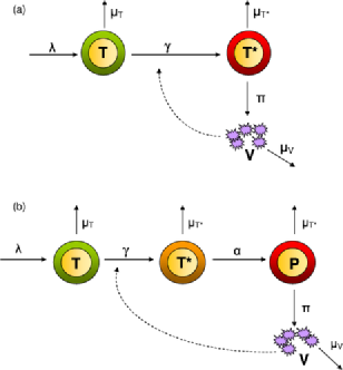
Figure 1: Graphical representation of “the basic model” (a) and “the productive cells model” (b).

Table 1: Parameters of the dynamic models

Parameter	Meaning (per day)	Value
$\lambda$	Rate of $T$ cell production per $\mu$L	estimated
$\mu_{T^{*}}$	Death rate of $T^{*}$ cells	estimated
$\pi$	Number of virions per $T^{*}$ cells	estimated
$\mu_{T}$	Death rate of $T$ cells	estimated
$\gamma$	Infection rate of $T$ cells per virion per $\mu$L	0.00027 [(Davenport et al., 2006);
		(Wilson et al., 2007)]
$\mu_{V}$	Clearance of free virions	20.0 [(Ramratnam et al., 1999)]
$\alpha$	Rate to become productive cells	1.0 [(Kiernan et al., 1990);
		(Barbosa et al., 1994)]

We assume that the model is at equilibrium before infection, so at $t=0_{-}$, we have

$$\cases{T_{0_{-}}=\displaystyle\frac{\lambda}{\mu_{T}},\cr T^{*}_{0_{-}}=0,\cr V_{0_{-}}=0.}$$

The initial inoculum of virions is fixed at $10^{-6}$ virions/mm³ [(Ciupe et al., 2006) (Stafford et al., 2000)], which is equivalent to 5 virions for 5 liters of blood. The introduction of virions in the system at $t=0$ disrupts the initial stability and the system stabilizes to a new equilibrium if the basic reproduction number $R_{0}$ ($R_{0}=\frac{\lambda\gamma\pi}{\mu_{T}\mu_{T^{*}}\mu_{V}}$) is higher than 1:

$$\cases{\bar{T}=\displaystyle\frac{\mu_{T^{*}}\mu_{V}}{\gamma\pi},\vspace*{2pt}\cr\bar{T}^{*}=\displaystyle\frac{\lambda\gamma\pi-\mu_{T}\mu_{T^{*}}\mu_{V}}{\gamma\pi\mu_{T^{*}}},\vspace*{2pt}\cr\bar{V}=\displaystyle\frac{\lambda\gamma\pi-\mu_{T}\mu_{T^{*}}\mu_{V}}{\gamma\mu_{T^{*}}\mu_{V}}.}$$

The second model (the “productive cells model”) distinguishes nonproductive infected cells ($T^{*}$) and productive infected cells ($P$) [Figure 1(b)] as previously suggested in (Nowak et al., 1997a). This second model includes one more parameter $\alpha$ (the rate to become productive infected cells). The model can be written as

$$\cases{\displaystyle\frac{dT}{dt}=\lambda-\gamma VT-\mu_{T}T,\vspace*{2pt}\cr\displaystyle\frac{dT^{*}}{dt}=\gamma VT-\mu_{T^{*}}T^{*}-\alpha T^{*},\vspace*{2pt}\cr\displaystyle\frac{dP}{dt}=\alpha T^{*}-\mu_{T^{*}}P,\vspace*{2pt}\cr\displaystyle\frac{dV}{dt}=\pi P-\mu_{V}V.}$$ (3)

The equilibrium before infection is

$$\cases{T_{0_{-}}=\displaystyle\frac{\lambda}{\mu_{T}},\vspace*{2pt}\cr T^{*}_{0_{-}}=0,\cr P_{0_{-}}=0,\cr V_{0_{-}}=0.}$$

After the introduction of virions, the system stabilizes to a new equilibrium if $R_{0}$ ($R_{0}=\frac{\lambda\gamma\pi\alpha}{\mu_{T}\mu_{T^{*}}\mu_{V}(\mu_{T^{*}}+\alpha)}$) is higher than 1:

$$\cases{\displaystyle\bar{T}=\frac{\mu_{T^{*}}\mu_{V}(\mu_{T^{*}}+\alpha)}{\gamma\pi\alpha},\cr\displaystyle\bar{T}^{*}=\frac{\lambda}{\mu_{T^{*}}+\alpha}-\frac{\mu_{T}\mu_{V}\mu_{T^{*}}}{\gamma\pi\alpha},\vspace*{2pt}\cr\displaystyle\bar{P}=\frac{\alpha}{\mu_{T^{*}}}\biggl{(}\frac{\lambda}{\mu_{T^{*}}+\alpha}-\frac{\mu_{T}\mu_{V}\mu_{T^{*}}}{\gamma\pi\alpha}\biggr{)},\vspace*{2pt}\cr\displaystyle\bar{V}=\frac{\pi\alpha}{\mu_{V}\mu_{T^{*}}}\biggl{(}\frac{\lambda}{\mu_{T^{*}}+\alpha}-\frac{\mu_{T}\mu_{V}\mu_{T^{*}}}{\gamma\pi\alpha}\biggr{)}.}$$

3.2 Statistical models

We can construct statistical models as in Section 2.1. We took $\Psi_{l}(\cdot)=\log(\cdot)$ for all $l$ to ensure positivity of parameters. The individual parameters are $\tilde{\bolds{\xi}}^{i}=(\tilde{\lambda}^{i},\tilde{\mu}_{T^{*}}^{i},\tilde{\pi}^{i},\tilde{\mu}_{T}^{i})$ with $\tilde{\lambda}^{i}=\log\lambda^{i}$, $\tilde{\mu}_{T^{*}}^{i}=\log\mu_{T^{*}}^{i}$, $\tilde{\pi}^{i}=\log\pi^{i}$ and $\tilde{\mu}_{T}^{i}=\log\mu_{T}^{i}$. Because of identifiability issues [(Wu et al., 2008)], the values of the other parameters were taken according to the literature: $\mu_{V}=20.0$ day^-1 [(Ramratnam et al., 1999)] and $\gamma=0.00027$ virions^-1 day^-1 $\mu$L^-1 [(Davenport et al., 2006); (Wilson et al., 2007)]. The parameter $\alpha$ is fixed at 1 day^-1 because the time lag between virus entry and virus production is about 1 day [(Kiernan et al., 1990); (Barbosa et al., 1994)].

The observed components were the base-10 logarithm of HIV RNA load (number of virions per $\mu$L) and the fourth root of total CD4 count (number of cells per $\mu$L). For the “basic model,” $g_{1}(X)=\log_{10}(V)$ and $g_{2}(X)=(T+T^{*})^{0.25}$ where $X=(T,T^{*},V)$. For the “productive cells model,” $g_{1}(X)=\log_{10}(V)$ and $g_{2}(X)=(T+T^{*}+P)^{0.25}$ where $X=(T,T^{*},P,V)$. These transformations are commonly used for achieving normality and homoscedasticity of measurement error distributions [(Thiébaut et al., 2003)]. We have

$$Y^{i}_{j1} = g_{1}(X(t^{i}_{j1},\tilde{\xi}^{i}))+\varepsilon^{i}_{j1},\qquad j=1,\ldots,n^{i}_{1},$$ (4)

$$Y^{i}_{j2} = g_{2}(X(t^{i}_{j2},\tilde{\xi}^{i}))+\varepsilon^{i}_{j2},\qquad j=1,\ldots,n^{i}_{2},$$ (5)

where $\varepsilon^{i}_{j1}$ and $\varepsilon^{i}_{j2}$ are independent Gaussian with zero mean and variances $\sigma_{\mathit{VL}}^{2}$ and $\sigma_{\mathit{CD}4}^{2}$ respectively.

3.3 Simulation study

We simulated samples of 100 subjects during primary HIV infection using the “basic model” for simplicity. The parameter values were defined according to the estimates of our application (see Tables 1 and 3). For each subject, we simulated the dates of HIV tests and the date of infection. Dates for the HIV serology tests (negative and positive, respectively) were simulated according to the prior distribution defined in Section 2.1 [equation (1)]. The subjects had a probability of 0.10 to have a short window of infection (90 days) with repeated measurements around the time of viral peak and a probability of 0.90 to have a window of infection of 200 days with repeated measurements after 150 days post-infection. The times of measurements $t^{i}_{jm}$ were as follows: days 1, 10, 15, 30, 50 and 100 for the short windows and days 150, 200, 240, 280, 300 and 350 for the others. We included independent random effects for the first two parameters ($\lambda$ and $\mu_{T^{*}}$). Therefore, the vector of parameters to be estimated was $(\tilde{\lambda}^{i},\tilde{\mu}_{T^{*}}^{i},\tilde{\pi}^{i},\tilde{\mu}_{T}^{i},\sigma_{\tilde{\lambda}},\sigma_{\tilde{\mu}_{T^{*}}},\sigma_{\mathit{VL}},\sigma_{\mathit{CD}4})$.

We performed a simulation study to compare the estimates according to three methods: (i) when the date of infection is fixed as the real date (RD) or (ii) when it is imputed at the midpoint of the interval defined the last negative and the first positive HIV test (DI) and (iii) when the uncertainty of the date of infection was taken into account with our proposed method (DUK). We simulated 50 data sets of 100 subjects with the design described above. For each data set, we estimated parameters with the three methods and we compared them by computing the mean square errors and the coverage rates (Table 2). The method using the real date of infection was used as a reference.

Table 2: Mean Square Errors (MSE) and coverage rates of the estimation method in the situations where the date of infection is known (RD), the date of infection is imputed at the midpoint (DI) and the uncertainty of the date of infection is taken into account (DUK)

	MSE			Coverage rate ($\bolds{\%}$)
Parameter	RD	DI	DUK	RD	DI	DUK
$\tilde{\lambda}$	0.0030	0.0498	0.0033	100	80	100
$\tilde{\mu}_{T^{*}}$	0.0098	0.1880	0.0086	100	90	100
$\tilde{\pi}$	0.0021	0.0426	0.0115	100	90	98
$\tilde{\mu}_{T}$	0.0065	4.0268	0.0023	100	60	100
$\sigma_{\tilde{\lambda}}$	0.0014	0.0079	0.0022	100	75	100
$\sigma_{\tilde{\mu}_{T^{*}}}$	0.0051	0.0143	0.0071	100	90	98
$\sigma_{\mathit{VL}}$	0.0011	0.0075	0.0007	100	100	100
$\sigma_{\mathit{CD}4}$	0.0001	0.0688	0.0001	100	100	100

[]$\sigma_{\tilde{\lambda}}$ and $\sigma_{\tilde{\mu}_{T^{*}}}$ are the standard deviations of random effect for $\tilde{\lambda}$ and $\tilde{\mu}_{T^{*}}$.
$\sigma_{\mathit{VL}}$ and $\sigma_{\mathit{CD}4}$ are the standard deviations of the observation error of $\log_{10}(V)$ and $(T+T^{*})^{0.25}$.

The DUK estimators had a much smaller MSE than the DI estimators and close to the MSE of the RD estimators. It is not feasible with such computationally demanding programs to make a large simulation. Fifty replications are not enough to precisely estimate coverage rates but are enough to show the superiority of our approach over the approach based on imputing the date of infection at midpoint. The empirical coverage rates were slightly too high for RD and DUK probably due to overestimation of the variance of the parameters.

4 Application to the CASCADE data set

4.1 The study sample

The study sample came from the Concerted Action on SeroConversion to AIDS and Death in Europe (CASCADE) study; it includes seroconverters from Europe, Canada and Australia. The CASCADE study has been described in detail elsewhere [(CASCADE, 2003)]. Data were pooled in the 2006 update from 20 participating cohorts. We selected HIV seroconverters if their HIV interval test (delay between the date of last seronegative test and the date of first seropositive test) was less than 3 years, if they did not receive any antiretroviral treatment during the first year following the date of seropositive test and if they had more than 3 measurements of CD4 or viral load during this first year of follow-up with the first detectable viral load measurement during the first three months after the date of seropositive test. A total of 761 patients met these criteria.

4.2 Models used

We used the two models defined in Section 3.1. The vector of natural parameters to be estimated for subject $i$ was $\xi^{i}=(\lambda^{i},\mu_{T^{*}}^{i},\break\pi^{i},\mu_{T}^{i})$ for the two models. The other parameters were assumed to be known as described in Section 3.2. The windows for possible dates of infection were fixed as defined in Section 2.2.

Random effects were selected according to a forward selection procedure. Starting with a model without random effect, we introduced random effects successively on each parameter and selected the one leading to the best likelihood improvement. Then, we added a new random effect and continued until the new model was not rejected by a likelihood ratio test.

4.3 Results

Selected patients had a median of four measurements for CD4 and for HIV RNA (InterQuartile Range [IQR$]=[$3; 5]). Most of the patients were infected by sex between men (71%). Follow-up was censored after 1 year beyond seropositive HIV test, resulting in a median follow-up after the first seropositive test of 195 days (IQR${}=[$119; 260]). The median of the delay between the dates of last seronegative and first seropositive test was 170 days (IQR${}=[$91; 273]).

The final models included independent random effects for the first two parameters. Therefore, the estimated vector of parameters was $(\tilde{\lambda},\tilde{\mu_{T^{*}}},\tilde{\pi},\tilde{\mu_{T}},\sigma_{\tilde{\lambda}},\break\sigma_{\tilde{\mu}_{T^{*}}},\sigma_{\mathit{VL}},\sigma_{\mathit{CD}4})$ for the two models. Usually, random effects are assumed to be independent in ODE models [(Putter et al., 2002); (Samson, Lavielle and Mentré, 2006); (Huang and Wu, 2006); (Guedj, Thiébaut and Commenges, 2007a)]. To test a possible correlation between the two random effects included in our models, we developed a score test based on our previous work [(Drylewicz, Commenges and Thiébaut, 2010)]. For both models, the test was not significant ($p=0.87$ and $p=0.92$, respectively). The score test is presented in Appendix A.

The “productive cells model” fitted better than the “basic model” (AIC${}={}$ 14,300 vs. 15,010). The improvement brought by this model can be considered as large according to the criterion $\mathrm{D}$ which is the difference of AIC divided by the total number of observations: $\mathrm{D}=\frac{15{,}010-14{,}300}{6294}=0.11$ [(Commenges et al., 2008)]. Estimates of the parameters of the two models are presented in Table 3.

=300pt Basic model Productive cells model Parameter Estimate SE Estimate SE $\tilde{\lambda}$ $-$3.49 0.032 $-$3.33 0.034 $\tilde{\mu_{T^{*}}}$ $-$0.62 0.046 $-$0.54 0.045 $\tilde{\pi}$ $-$5.27 0.041 $-$6.06 0.036 $\tilde{\mu_{T}}$ $-$3.26 0.019 $-$3.40 0.034 $\sigma_{\tilde{\lambda}}$ $-$0.16 0.008 $-$0.41 0.057 $\sigma_{\tilde{\mu}_{T^{*}}}$ $-$0.42 0.043 $-$0.37 0.052 $\sigma_{\mathit{VL}}$ $-$0.82 0.017 $-$0.75 0.017 $\sigma_{\mathit{CD}4}$ $-$0.29 0.012 $-$0.27 0.013 AIC 15,010 14,300 []$\sigma_{\tilde{\lambda}}$ and $\sigma_{\tilde{\mu}_{T^{*}}}$ are the standard deviations of random effect for $\tilde{\lambda}$ and $\tilde{\mu}_{T^{*}}$.$\sigma_{\mathit{VL}}$ and $\sigma_{\mathit{CD}4}$ are the standard deviations of the observation error of $\log_{10}(V)$ and $(T+T^{*})^{0.25}$ for the “basic model” and $(T+T^{*}+P)^{0.25}$ for the “productive cells model.”

Table 3: Estimated parameters and standard-errors (SE) on logarithmic scale for the “basic” and the “productive cells” models; for meaning of parameters see Table 1

For the “productive cells model,” on the natural scale, the mean half-life [$\log(2)/$Death rate] of infected and uninfected cells was 0.40 and 21 days, respectively. At the time of the viral peak (median viral load of 5.68 $\log_{10}$ copies/mL, $\mathrm{IQR}=[5.44;5.96]$), the estimated median number of infected cells was 64 cells/$\mu$L ($\mathrm{IQR}=[40;113]$). At the same time, the median number of productive cells/$\mu$L was 24 ($\mathrm{IQR}=[14;46]$) among 557 CD4 cells/$\mu$L ($\mathrm{IQR}=[460;658]$). The median of the estimated CD4 setpoints was 500 cells/$\mu$L ($\mathrm{IQR}=[396;627]$) which is close to the median of observed setpoints (based on at least one measurement after 365 days available in 430 patients): 470 cells/$\mu$L ($\mathrm{IQR}=[371;615]$). At the same time, the median of the estimated number of infected cells/$\mu$L was 8 ($\mathrm{IQR}=[6;12]$) including a median of 3 productive cells/$\mu$L ($\mathrm{IQR}=[2;5]$). The median of viral setpoints was also close to that observed in 403 patients: 4.77 $\log_{10}$ copies/mL ($\mathrm{IQR}=[4.59;4.98]$) vs. 4.59 ($\mathrm{IQR}=[4.04;5.00]$).

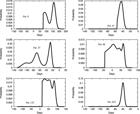
Figure 2: A posteriori individual distributions of the date of infection for patients 6, 41, 55, 66, 132 and 652 from the “productive cells model,” where day 0 is the date of last negative HIV test.

We found very different a posteriori individual distributions of the date of infection depending on the width of the window and the quantity of available information for each patient. Figure 2 shows the a posteriori distributions displayed on the window of infection (see Section 2.2), where 0 represents the last seronegative date for six patients chosen for exhibiting different shapes of the a posteriori distribution. For patients with data clearly before the setpoint, the model was able to restrict the possible dates of infection. For instance, patient 132 had an interval of possible dates of infection of 273 days and our estimation restricted this interval to 90 days. However, for other patients and especially for some patients with a wide interval between last negative and first positive HIV serology test, the a posteriori distribution had local maxima. Analysis of marker dynamics according to the local maxima suggested quite different possibilities according to the available information (Figure 3).

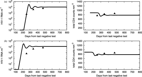
Figure 3: Predicted fits from the two most probable dates of infection [(a) the global maximum and (b) the local maximum] and observed values of HIV RNA level and total CD4 count for patient 6 from the “productive cells model.”

For each patient, we took the date with the highest probability and plotted predicted individual trajectories for each marker from this date. The fits of the model were satisfactory. The estimated trajectories are in agreement with those reported in the literature [(Little et al., 1999); (Lindback et al., 2000); (Stafford et al., 2000)]. Individual predicted fits and observed values are shown in Figure 4 for six patients. We studied the distribution of residuals and the agreement between predictions and observations for plasma HIV RNA and CD4 count in Appendix B.

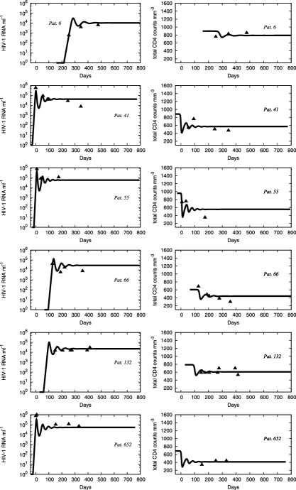
Figure 4: Individual predicted fits from the most probable date of infection and observed values of HIV RNA level and total CD4 count for patients 6, 41, 55, 66, 132 and 652 from the “productive cells model,” where day 0 is the date of last negative HIV test.

5 Discussion

In this paper we present a method for estimating parameters of random effects models based on differential equations when the origin of time is unknown, taking also into account unbalanced data and left-censored observations. This method was applied to a cohort of HIV patients during primary infection using repeated measurements of two markers: plasma HIV RNA and CD4$+$ T cell counts. The model gave reasonable fits although the kinetics of the markers was very complex due to nonlinear interaction between the virus and the target cells. Thanks to the population approach, we were able to describe the dynamics of markers during primary infection using data from several hundred patients.

Predictions were obviously driven by the structure of the ODE system that is based on biological knowledge. Compared to a descriptive model, this mechanistic approach brings additional information. Typically, solutions of ODE systems led to oscillatory trajectories [(Volterra, 1926)]: these oscillations are dampened as time passes so that the trajectory gets closer to the steady state value. Observations are partly consistent with the oscillating behavior. The peak of viral load, the reality of which is generally admitted, is nothing but the first oscillation. It can be noted that the oscillations are generally more dampened for more complex systems [(Burg et al., 2009)]. In conclusion, the oscillatory trajectories produced by our model are for a part the expression of a real phenomenon.

Predicted viral and CD4 setpoints (defined as markers values at equilibrium) were quite similar to those that could be observed. Interestingly, the estimated value of infected cells (that are not observed) was in agreement with previous studies reporting a low concentration of productive infected cells [(Chun et al., 1997)].

Because the approach was based on a mechanistic model, the parameters have biological meanings. For instance, the mean half-life of infected cells was estimated at 0.40 day. Previous estimations of this parameter were mainly performed in patients treated by antiretroviral therapy. These estimations varied from 0.7 day to 1.8 day according to the type of treatment and the type of model used [(Perelson et al., 1996); (Faulkner et al., 2003); (Huang and Wu, 2006); (Huang, 2007)]. Similarly, it is interesting to note that our estimate of virus production (428 virions/cell/day) is of the same order as what has been reported [(Dimitrov et al., 1993); (Levy et al., 1996); (Haase, 1999)]. However, the biological relevance of the present model could still be questioned with regards to other processes that have been ignored. For instance, the cytotoxic T-cell response plays a role in the control of the infection and the decrease of the viral load by killing the infected cells [(Stafford et al., 2000)], although the efficiency of this immunological response is debated [(Asquith and McLean, 2007)]. Moreover, our estimate of target CD4 cells half-life is a mixture of the half-life of quiescent cells and that of activated cells [(Mclean and Michie, 1995); (Vrisekoop et al., 2008)].

The uncertainty on the date of infection was taken into account to improve the accuracy of the estimates as compared to performing simple imputations. In addition, we were able to derive the individual posterior distribution of the date of infection according to the model. When enough information is available the date of infection can be estimated with good accuracy (Figure 2). The sensitivity of the estimates to the assumptions about the priors [equation (1) in Section 2.2] was roughly proportional to the amount of data available as illustrated by the posterior infection time distribution of patient 41 compared to patient 66 (Figure 2). We also performed a sensitivity analysis which demonstrated a certain robustness of the method. The lower bound of the infection time distribution could be better defined by using additional information such as antibody dynamics. Unfortunately, this information was not available in the present data set.

The main limitation for the use of dynamical models is the parameter identifiability that led us to fix the value of $\gamma$ (infection rate) and $\mu_{V}$ (viral clearance). The clearance was fixed to 20 day^-1 according to recent studies with highly repeated measures of HIV RNA after initiation of antiretroviral treatment [(Perelson et al., 1997); (Ramratnam et al., 1999)]. The chosen value of $\mu_{V}$ may influence the estimation of other parameters such as $\pi$, as the viral setpoint is essentially determined by the ratio $\frac{\pi}{\mu_{V}}$ [(Nowak et al., 1997a)]. Identifiability may be improved by measuring more compartments such as infected cells or by increasing the number of repeated measurements [(Guedj, Thiébaut and Commenges, 2007b)]. This is an important point to consider in future studies, as the issue of identifiability precludes the comparison with more complex models.

Finally, this method can be applied in other areas where either the model is simpler or the amount of measured information greater, so that identifiability is less an issue.

Table 4: Notation used in the manuscript

Notation	Meaning
$i$ $(1,\ldots,n)$	Subject
$X^{i}(t)$	Vector of the $K$ components of the model at time $t$
$\xi^{i}$	Vector of $p$ individual natural parameters
$\tilde{\xi}^{i}=\Psi(\xi^{i})$	Vector of $p$ individual transformed parameters
$\phi_{l}$	Intercept of the $l$th parameter
$z^{i}_{l}$	Vectors of explanatory variables associated to the fixed effects of the $l$th
	biological parameter
$\beta_{l}^{i}$	Vectors of regression coefficients associated to the fixed effects
$b^{i}=Au^{i}$	Individual vector of random effects of dimension $q$
$A=(a_{l^{\prime\prime}l^{\prime}})_{l^{\prime}\leq l^{\prime\prime}\leq q}$	Lower triangular matrix with positive diagonal elements $AA^{\prime}=\Sigma$
	(Cholesky decomposition)
$Y^{i}_{jm}$	$j$th measurement of the $m$th compartment of subject $i$
$d^{i}_{jm}$	Date of measurement of $Y^{i}_{jm}$
$\tau^{i}$	Date of infection of subject $i$
$t^{i}_{jm}$	Time between $\tau^{i}$ and $d^{i}_{jm}$
$g_{m}(\cdot)$ $(m=1,\ldots,M)$	Nonlinear function for the $m$th observed compartment
$\varepsilon^{i}_{jm}$	Gaussian measurement errors with zero mean and variances $\sigma_{m}^{2}$
$d^{i}_{-}$	Date of last negative HIV test of subject $i$
$d^{i}_{+}$	Date of first positive HIV test of subject $i$
$f_{\tau^{i}}$	Density of infection date $\tau^{i}$
$[\tau_{\inf}^{i},\tau_{\sup}^{i}]$	Support of the density $f_{\tau^{i}}$
$\zeta^{i}_{j}$	Detection limit of the $j$th measurement of subject $i$

Appendix A Score test for covariance of random effects

In (Drylewicz, Commenges and Thiébaut, 2010), we have developed score tests for explanatory variables and variance of random effects in complex models. We propose here to develop a test for the covariance parameter of random effects. We assume that the date of infection is known and introduce notation for a conventional nonlinear model. For subject $i$ with $i=1,\ldots,n$, we consider a model which specifies the distribution of the observed vector ${\mathbf{Y}}^{i}=(Y^{i}_{j},j=1,\ldots,n^{i})$:

$$Y^{i}_{j}=g(t^{i}_{j},\tilde{\bolds{\xi}}^{i})+\varepsilon^{i}_{j},\qquad j=1,\ldots,n^{i},$$

where $Y^{i}_{j}$ is the $j$th measurement for subject $i$ at the time $t^{i}_{j}$, and the $\varepsilon^{i}_{j}$ are independent Gaussian measurement errors with zero mean and variances $\sigma^{2}$. The function $g(\cdot)$ is a twice differentiable (generally nonlinear) function. The individual parameters $\tilde{\bolds{\xi}}^{i}=(\tilde{\xi_{l}}^{i},l=1,\ldots,p)$ are modeled as a linear form: $\tilde{\xi}_{l}^{i}=\phi_{l}+b^{i}_{l}+z_{l}^{i}\bolds{\beta}_{l}$, where $\phi_{l}$ is the intercept, and $z^{i}_{l}$ is the vector of explanatory variables associated to the fixed effects of the $l$th parameter. The $\bolds{\beta}_{l}$’s are vectors of regression coefficients. We assume $b^{i}\sim\mathcal{N}(0,\Sigma)$, where $b^{i}$ is the individual vector of random effects of dimension $q$. Let $A=(a_{l^{\prime\prime}l^{\prime}})_{l^{\prime}\leq l^{\prime\prime}\leq q}$ be the lower triangular matrix with positive diagonal elements such that $AA^{\prime}=\Sigma$ (Cholesky decomposition). We can write $b^{i}=A\mathbf{u}^{i}$ with $\mathbf{u}^{i}\sim\mathcal{N}(\mathbf{0},\mathbf{I}_{q})$. We denote by $\bolds{\theta}=(\phi_{l},A,\beta_{l},l=1,\ldots,p)$ the set of parameters of the model and by $\mathcal{L}^{\theta}_{\mathcal{Y}^{i}|u^{i}}(Y^{i}|{\mathbf{u}})$ the likelihood of observations for subject $i$ given that the random effects ${\mathbf{u}}^{i}$ take the value $\mathbf{u}$. Given ${\mathbf{u}}^{i}$, the $Y^{i}_{j}$ are independent, so $\mathcal{L}^{\theta}_{\mathcal{Y}^{i}|u^{i}}(Y^{i}|{\mathbf{u}})=\prod_{j}\mathcal{L}^{\theta}_{\mathcal{Y}^{i}_{j}|u^{i}}(Y^{i}_{j}|{\mathbf{u}})$, where

$$\mathcal{L}^{\theta}_{\mathcal{Y}^{i}_{j}|u^{i}}(Y^{i}_{j}|{\mathbf{u}})=\frac{1}{\sqrt{2\pi}\sigma}\exp\biggl{\{}-\frac{(Y^{i}_{j}-g(t^{i}_{j},\tilde{\bolds{\xi}}^{i}))^{2}}{2\sigma^{2}}\biggr{\}}.$$

The observed log-likelihood for subject $i$ is

$$L^{\theta}_{i}=\log\int_{\mathbb{R}^{q}}\mathcal{L}^{\theta}_{\mathcal{Y}^{i}|u^{i}}(Y^{i}|{\mathbf{u}})\phi(\mathbf{u})\,d\mathbf{u},$$

where $\phi$ is the multivariate normal density of $\mathcal{N}({\mathbf{0}},{\mathbf{I}}_{q})$. We denote $L=L^{\theta}_{1}+\cdots+L^{\theta}_{n}$, the global log-likelihood.

For simplicity and for illustrating our specific case, we assume that only two random effects are included in the model ($u_{l}^{i}$ and $u_{l^{\prime}}^{i}$). We want to test whether $b_{l}^{i}$ and $b_{l^{\prime}}^{i}$ are independent. The null hypothesis $H_{0}$ is “$a_{ll^{\prime}}=0$”. The scores $U_{ll^{\prime}}^{i}$ (individual score for $a_{ll^{\prime}}$) are obtained integrating $U_{ll^{\prime}|u^{i}}^{i}$ using Louis’ formula [(Louis, 1982)]:

$$U_{ll^{\prime}}^{i}=(\mathcal{L}_{\mathcal{O}^{i}})^{-1}\int_{\mathbb{R}^{2}}\mathcal{L}^{\theta}_{\mathcal{Y}^{i}|u^{i}}({\mathbf{u}})U_{ll^{\prime}|u^{i}}^{i}({\mathbf{u}})\phi({\mathbf{u}})\,d{\mathbf{u}},$$

where

$$U_{ll^{\prime}|u^{i}}^{i}(\mathbf{u})=\sum_{j=1,n^{i}}\frac{1}{\sigma^{2}}\bigl{(}Y^{i}_{j}-g(X(t^{i}_{j},\tilde{\bolds{\xi}^{i}}))\bigr{)}\biggl{(}u_{l^{\prime}}^{i}a_{ll}\frac{\partial g(X(t^{i}_{j},\tilde{\bolds{\xi}^{i}}))}{\partial\bolds{\xi}^{i}_{l}}\biggr{)}.$$

Under the null hypothesis, we propose the following statistic:

$$S=\frac{U^{\bullet}_{ll^{\prime}|H_{0}}}{\sqrt{\widehat{\operatorname}{Var}U^{\bullet}_{ll^{\prime}|H_{0}}}},$$

where $U^{\bullet}_{ll^{\prime}|H_{0}}$ is the sum of individual scores $U_{ll^{\prime}}^{i}$ calculated under $H_{0}$ and $\widehat{\operatorname}{Var}\,{U^{\bullet}_{ll^{\prime}|H_{0}}}$ is a consistent estimator of $\operatorname{Var}{U^{\bullet}_{ll^{\prime}|H_{0}}}$. $S$ has an asymptotic standard normal distribution under $H_{0}$. We take $\widehat{\operatorname}{Var}\,{U^{\bullet}_{ll^{\prime}|H_{0}}}=\sum_{i=1,n}{U^{i2}_{ll^{\prime}|H_{0}}}$.

Appendix B Goodness of fit

Figures 5 and 6 present the residuals with respect to the predictions and the observations with respect to the predictions for the fourth root of CD4 count and the base 10-logarithm of HIV RNA load. The residuals are computed using empirical bayes and predictions from the most probable date of infection for each patient. We excluded left-censored HIV RNA measurements (72 among 3038 measurements).

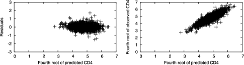
Figure 5: Residuals of fourth-root of CD4 count with respect to predictions (left) and observations with respect to predictions (right).

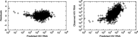
Figure 6: Residuals of HIV RNA with respect to predictions (left) and observations with respect to predictions (right), the left-censored measurements of HIV RNA have been excluded (72 among 3038 measurements).

The residuals are well distributed around 0 and there is a good agreement between predictions and observations for both HIV RNA and CD4 count. The four outliers observed on the left of HIV RNA figures are due to patients having only one detectable measurement of HIV RNA during their follow-up and the only detectable value was low ($<$$3\log_{10}$ copies/mL).

CASCADE collaboration

Steering Committee: Julia Del Amo (Chair), Laurence Meyer (Vice Chair), Heiner Bucher, Geneviève Chêne, Deenan Pillay, Maria Prins, Magda Rosinska, Caroline Sabin, Giota Touloumi.

Co-ordinating Centre: Kholoud Porter (Project Leader), Sara Lodi, Sarah Walker, Abdel Babiker, Janet Darbyshire.

Clinical Advisory Board: Heiner Bucher, Andrea de Luca, Martin Fisher, Roberto Muga.

Collaborators: Australia Sydney AIDS Prospective Study and Sydney Primary HIV Infection cohort (John Kaldor, Tony Kelleher, Tim Ramacciotti, Linda Gelgor, David Cooper, Don Smith); Canada South Alberta clinic (John Gill); Denmark Copenhagen HIV Seroconverter Cohort (Louise Bruun Jorgensen, Claus Nielsen, Court Pedersen); Estonia Tartu Ulikool (Irja Lutsar); France Aquitaine cohort (Geneviève Chêne, Francois Dabis, Rodolphe Thiébaut, Bernard Masquelier), French Hospital Database (Dominique Costagliola, Marguerite Guiguet), Lyon Primary Infection cohort (Philippe Vanhems), SEROCO cohort (Laurence Meyer, Faroudy Boufassa); Germany German cohort (Osamah Hamouda, Claudia Kucherer); Greece Greek Haemophilia cohort (Giota Touloumi, Nikos Pantazis, Angelos Hatzakis, Dimitrios Paraskevis, Anastasia Karafoulidou); Italy Italian Seroconversion Study (Giovanni Rezza, Maria Dorrucci, Benedetta Longo, Claudia Balotta); Netherlands Amsterdam Cohort Studies among homosexual men and drug users (Maria Prins, Liselotte van Asten, Akke van der Bij, Ronald Geskus, Roel Coutinho); Norway Oslo and Ulleval Hospital cohorts (Mette Sannes, Oddbjorn Brubakk, Anne Eskild, Johan N. Bruun); Poland National Institute of Hygiene (Magdalena Rosinska); Portugal Universidade Nova de Lisboa (Ricardo Camacho); Russia Pasteur Institute (Tatyana Smolskaya); Spain Badalona IDU hospital cohort (Roberto Muga), Barcelona IDU Cohort (Patricia Garcia de Olalla), Madrid cohort (Julia Del Amo, Jorge del Romero), Valencia IDU cohort (Santiago Pérez-Hoyos, Ildefonso Hernandez Aguado); Switzerland Swiss HIV cohort (Heiner Bucher, Martin Rickenbach, Patrick Francioli); Ukraine Perinatal Prevention of AIDS Initiative (Ruslan Malyuta); United Kingdom Edinburgh Hospital cohort (Ray Brettle), Health Protection Agency (Valerie Delpech, Sam Lattimore, Gary Murphy, John Parry, Noel Gill), Royal Free haemophilia cohort (Caroline Sabin, Christine Lee), UK Register of HIV Seroconverters (Kholoud Porter, Anne Johnson, Andrew Phillips, Abdel Babiker, Janet Darbyshire, Valerie Delpech), University College London (Deenan Pillay), University of Oxford (Harold Jaffe).

References

- Anderson and May (1991) Anderson, R. and May, R. (1991). Infectious Diseases of Humans. Oxford Univ. Press.
- Asquith and McLean (2007) Asquith, B. and McLean, A. (2007). In vivo CD8 T cell control of immunodeficiency virus infection in humans and macaques. Proc. Natl. Acad. Sci. USA 104 6365–6370.
- Barbosa et al. (1994) Barbosa, P., Charneau, P., Dumey, N. and Clavel, F. (1994). Kinetic analysis of HIV-1 early replicative steps in a coculture system. AIDS Research and Human Retroviruses 10 53–59.
- Berlizov and Zhmudsky (1999) Berlizov, A. and Zhmudsky, A. (1999). The recursive adaptive quadrature in MS Fortran-77. Arxiv preprint. Available at arXiv:physics/9905035.
- Berman (1990) Berman, S. (1990). A stochastic model for the distribution of HIV latency time based on T4 counts. Biometrika 77 733–741.
- Burg et al. (2009) Burg, D., Rong, L., Neumann, A. and Dahari, H. (2009). Mathematical modeling of viral kinetics under immune control during primary HIV-1 infection. J. Theoret. Biol. 259 751–759.
- Cao, Fussmann and Ramsay (2008) Cao, J., Fussmann, G. and Ramsay, J. (2008). Estimating a predator–prey dynamical model with the parameter cascades method. Biometrics 64 959–967. \MR2526648
- CASCADE (2003) CASCADE, C. (2003). Determinants of survival following HIV-1 seroconversion after the introduction of HAART: Results from CASCADE. The Lancet 362, 9392, 1267–1274.
- Chun et al. (1997) Chun, T., Carruth, L., Shen, X., Taylor, H. et al. (1997). Quantification of latent tissue reservoirs and total body viral load in HIV-1 infection. Nature 387 183–188.
- Ciupe et al. (2006) Ciupe, M., Bivort, B., Bortz, D. and Nelson, P. (2006). Estimating kinetic parameters from HIV primary infection data through the eyes of three different mathematical models. Math. Biosci. 200 1–27. \MR2211925
- Commenges et al. (2006) Commenges, D., Jacqmin-Gadda, H., Proust, C. and Guedj, J. (2006). A Newton-like algorithm for likelihood maximization: The robust variance scoring algorithm. Available at arXiv:math.ST/0610402.
- Commenges et al. (2008) Commenges, D., Sayyareh, A., Letenneur, L., Guedj, J. and Bar-Hen, A. (2008). Estimating a difference of Kullback–Leibler risks using a normalized difference of AIC. Ann. Appl. Statist. 2 1123–1142.
- Davenport et al. (2006) Davenport, M., Zhang, L., Shiver, J., Casmiro, D., Ribeiro, R. and Perelson, A. (2006). Influence of peak viral load on the extent of CD4 T-cell depletion in simian HIV infection. JAIDS Journal of Acquired Immune Deficiency Syndromes 41 259.
- De Boer and Perelson (1998) De Boer, R. and Perelson, A. (1998). Target cell limited and immune control models of HIV infection: A comparison. J. Theoret. Biol. 190 201–214.
- DeGruttola, Lange and Dafni (1991) DeGruttola, V., Lange, N. and Dafni, U. (1991). Modeling the progression of HIV infection. J. Amer. Statist. Assoc. 86 569–577.
- Desquilbet et al. (2004) Desquilbet, L., Goujard, C., Rouzioux, C., Sinet, M., Chaix, M., Sereni, D., Boufassa, F., Delfraissy, J., Meyer, L., PRIMO and Groups, S. S. (2004). Does transient HAART during primary HIV-1 infection lower the virological set-point? AIDS 18 2361–2369.
- Dimitrov et al. (1993) Dimitrov, D., Willey, R., Sato, H., Chang, L., Blumenthal, R. and Martin, M. (1993). Quantitation of human immunodeficiency virus type 1 infection kinetics. Journal of Virology 67 2182–2190.
- Drylewicz, Commenges and Thiébaut (2010) Drylewicz, J., Commenges, D. and Thiébaut, R. (2010). Score tests for exploring complex models: Application to HIV dynamical models. Biometrical Journal 52 10–21.
- Dubin et al. (1994) Dubin, N., Berman, S., Marmor, M., Tindall, B., Des Jarlais, D. and Kim, M. (1994). Estimation of time since infection using longitudinal disease-marker data. Stat. Med. 13 231–244.
- Faulkner et al. (2003) Faulkner, N., Lane, B., Bock, P. and Markovitz, D. (2003). Protein phosphatase 2A enhances activation of human immunodeficiency virus type 1 by phorbol myristate acetate. Journal of Virology 77 2276–2281.
- Fellay et al. (2007) Fellay, J., Shianna, K., Ge, D., Colombo, S., Ledergerber, B., Weale, M., Zhang, K., Gumbs, C., Castagna, A., Cossarizza, A. et al. (2007). A whole-genome association study of major determinants for host control of HIV-1. Science 317 944–947.
- Fidler et al. (2007) Fidler, S., Fox, J., Touloumi, G., Pantazis, N., Porter, K., Babiker, A., Weber, J. et al. (2007). Slower CD4 cell decline following cessation of a 3 month course of HAART in primary HIV infection: Findings from an observational cohort. AIDS 21 1283–1291.
- Fidler et al. (2006) Fidler, S., Fraser, C., Fox, J., Tamm, N., Griffin, J. and Weber, J. (2006). Comparative potency of three antiretroviral therapy regimes in primary HIV infection. AIDS 20 247–252.
- Fiebig et al. (2003) Fiebig, E., Wright, D., Rawal, B., Garrett, P., Schumacher, R., Peddada, L., Heldebrant, C., Smith, R., Conrad, A., Kleinman, S. et al. (2003). Dynamics of HIV viremia and antibody seroconversion in plasma donors: Implications for diagnosis and staging of primary HIV infection. AIDS 17 1871–1879.
- Filter, Xia and Gray (2005) Filter, R., Xia, X. and Gray, C. (2005). Dynamic HIV/AIDS parameter estimation with application to a vaccine readiness study in Southern Africa. IEEE Transactions on Biomedical Engineering 52 784–791.
- Geskus (2000) Geskus, R. (2000). On the inclusion of prevalent cases in HIV/AIDS natural history studies through a marker-based estimate of time since seroconversion. Stat. Med. 19 1753–1769.
- Geskus et al. (2007) Geskus, R., Prins, M., Hubert, J., Miedema, F., Berkhout, B., Rouzioux, C., Delfraissy, J. and Meyer, L. (2007). The HIV RNA setpoint theory revisited. Retrovirology 4 65–74.
- Guedj, Thiébaut and Commenges (2007a) Guedj, J., Thiébaut, R. and Commenges, D. (2007a). Maximum likelihood estimation in dynamical models of HIV. Biometrics 63 1198–1206. \MR2414598
- Guedj, Thiébaut and Commenges (2007b) Guedj, J., Thiébaut, R. and Commenges, D. (2007b). Practical identifiability of HIV dynamics models. Bull. Math. Biol. 69 2493–2513. \MR2353843
- Haase (1999) Haase, A. (1999). Population biology of HIV-1 infection: Viral and CD4 T cell demographics and dynamics in lymphatic tissues. Annual Reviews in Immunology 17 625–656.
- Hecht et al. (2006) Hecht, F., Wang, L., Collier, A., Little, S., Markowitz, M., Margolick, J., Kilby, J., Daar, E., Conway, B., Holte, S. et al. (2006). A multicenter observational study of the potential benefits of initiating combination antiretroviral therapy during acute HIV infection. Journal of Infectious Diseases 194 725–733.
- Huang (2007) Huang, Y. (2007). Modeling the short-, middle- and long-term viral load responses for comparing estimated dynamic parameters. Biometrical Journal 49 429–440. \MR2380523
- Huang, Liu and Wu (2006) Huang, Y., Liu, D. and Wu, H. (2006). Hierarchical Bayesian methods for estimation of parameters in a longitudinal HIV dynamic system. Biometrics 62 413–423. \MR2227489
- Huang and Wu (2006) Huang, Y. and Wu, H. (2006). A Bayesian approach for estimating antiviral efficacy in HIV dynamic models. J. Appl. Statist. 33 155–174. \MR2223142
- Kaufmann et al. (1998) Kaufmann, G., Cunningham, P., Kelleher, A., Zaunders, J., Carr, A., Vizzard, J., Law, M., Cooper, D. et al. (1998). Patterns of viral dynamics during primary human immunodeficiency virus type 1 infection. Journal of Infectious Diseases 178 1812–1815.
- Kiernan et al. (1990) Kiernan, R., Marshall, J., Bowers, R., Doherty, R. and McPhee, D. (1990). Kinetics of HIV-1 replication and intracellular accumulation of particles in HTLV-I-transformed cells. AIDS Research and Human Retroviruses 6 743–752.
- Levy et al. (1996) Levy, J., Ramachandran, B., Barker, E., Guthrie, J., Elbeik, T. and Coffin, J. (1996). Plasma viral load, CD4+ cell counts, and HIV-1 production by cells. Science 271 670–671.
- Lindback et al. (2000) Lindback, S., Karlsson, A., Mittler, J., Blaxhult, A., Carlsson, M., Briheim, G., Sonnerborg, A. and Gaines, H. (2000). Viral dynamics in primary HIV-1 infection. Karolinska institutet primary HIV infection study group. AIDS 14 2283–2291.
- Little et al. (1999) Little, S., McLean, A., Spina, C., Richman, D. and Havlir, D. (1999). Viral dynamics of acute HIV-1 infection. Journal of Experimental Medicine 190 841–850.
- Louis (1982) Louis, T. (1982). Finding the observed Information matrix when using the algorithm. J. Roy. Statist. Soc. Ser. B 44 226–233. \MR0676213
- Mclean and Michie (1995) McLean, A. and Michie, C. (1995). In vivo estimates of division and death rates of human t lymphocytes. Proc. Natl. Acad. Sci. USA 92 3707–3711.
- Mellors et al. (1995) Mellors, J., Kingsley, L., Rinaldo, C., Todd, J., Hoo, B., Kokka, R. and Gupta, P. (1995). Quantitation of HIV-1 RNA in plasma predicts outcome after seroconversion. Annals of Internal Medicine 122 573–579.
- Munoz et al. (1992) Munoz, A., Carey, V., Taylor, J., Chmiel, J., Kingsley, L., Van Raden, M. and Hoover, D. (1992). Estimation of time since exposure for a prevalent cohort. Stat. Med. 11 939–952.
- Murray et al. (1998) Murray, J., Kaufmann, G., Kelleher, A. and Cooper, D. (1998). A model of primary HIV-1 infection. Mathematical Biosciences 154 57–85.
- Nowak et al. (1997a) Nowak, M., Bonhoeffer, S., Shaw, G. and May, R. (1997a). Anti-viral drug treatment: Dynamics of resistance in free virus and infected cell populations. Journal of Theoretical Biology 184 203–217.
- Nowak et al. (1997b) Nowak, M., Lloyd, A., Vasquez, G., Wiltrout, T., Wahl, L., Bischofberger, N., Williams, J., Kinter, A., Fauci, A., Hirsch, V. et al. (1997b). Viral dynamics of primary viremia and antiretroviral therapy in simian immunodeficiency virus infection. Journal of Virology 71 7518–7525.
- Pantazis et al. (2005) Pantazis, N., Touloumi, G., Walker, A. and Babiker, A. (2005). Bivariate modelling of longitudinal measurements of two human immunodeficiency type 1 disease progression markers in the presence of informative drop-outs. J. Roy. Statist. Soci. Ser. C 54 405–423. \MR2135882
- Perelson (2002) Perelson, A. (2002). Modelling viral and immune system dynamics. Nature Reviews Immunology 2 28–36.
- Perelson et al. (1997) Perelson, A., Essunger, P., Cao, Y., Vesanen, M., Hurley, A., Saksela, K., Markowitz, M. and Ho, D. (1997). Decay characteristics of HIV-1-infected compartments during combination therapy. Nature 387 188–191.
- Perelson et al. (1996) Perelson, A., Neumann, A., Markowitz, M., Leonard, J. and Ho, D. (1996). Viral dynamics in human immunodeficiency virus type 1 infection. Science 271, 1582–1586.
- Phillips (1996) Phillips, A. (1996). Reduction of HIV concentration during acute infection: Independence from a specific immune response. Science 271 497–499.
- Putter et al. (2002) Putter, H., Heisterkamp, S., Lange, J. and de Wolf, F. (2002). A Bayesian approach to parameter estimation in HIV dynamical models. Stat. Med. 21 2199–2214.
- Ramratnam et al. (1999) Ramratnam, B., Bonhoeffer, S., Binley, J., Hurley, A., Zhang, L., Mittler, J., Markowitz, M., Moore, J., Perelson, A. and Ho, D. (1999). Rapid production and clearance of HIV-1 and hepatitis C virus assessed by large volume plasma apheresis. The Lancet 354 1782–1786.
- Ribeiro et al. (2010) Ribeiro, R., Qin, L., Chavez, L., Li, D., Self, S. and Perelson, A. (2010). Estimation of the initial viral growth rate and the basic reproductive number during acute HIV-1 infection. Journal of Virology 84 6096–6102.
- Samson, Lavielle and Mentré (2006) Samson, A., Lavielle, M. and Mentré, F. (2006). Extension of the SAEM algorithm to left-censored data in nonlinear mixed-effects model: Application to HIV dynamics model. Comput. Statist. Data Anal. 51 1562–1574. \MR2307526
- Stafford et al. (2000) Stafford, M., Cao, Y., Ho, D., Corey, L. and Perelson, A. (2000). Modeling plasma virus concentration and CD4 T cell kinetics during primary HIV infection. Journal of Theoretical Biology 203 285–301.
- Thiébaut et al. (2006) Thiébaut, R., Guedj, J., Jacqmin-Gadda, H., Chêne, G., Trimoulet, P., Neau, D. and Commenges, D. (2006). Estimation of dynamical model parameters taking into account undetectable marker values. BMC Medical Research Methodology 6 1–10.
- Thiébaut et al. (2003) Thiébaut, R., Jacqmin-Gadda, H., Leport, C., Katlama, C., D., C., Le Moing, V., Morlat, P., Chene, G. and the APROCO Study Group (2003). Bivariate longitudinal model for the analysis of the evolution of HIV RNA and CD4 cell count in HIV infection taking into account left censoring of HIV RNA measures. Journal of Biopharmaceutical Statistics 13 271–282.
- Volterra (1926) Volterra, V. (1926). Fluctuations in the abundance of a species considered mathematically. Nature 118 558–560.
- Vrisekoop et al. (2008) Vrisekoop, N., den Braber, I., de Boer, A., Ruiter, A., Ackermans, M., van der Crabben, S., Schrijver, E., Spierenburg, G., Sauerwein, H., Hazenberg, M. et al. (2008). Sparse production but preferential incorporation of recently produced naïve T cells in the human peripheral pool. Proc. Natl. Acad. Sci. 105 6115–6120.
- Wick (1999) Wick, D. (1999). The disappearing CD4 T cells in HIV infection: A case of over-stimulation? Journal of Theoretical Biology 197 507–516.
- Wilson et al. (2007) Wilson, D., Mattapallil, J., Lay, M., Zhang, L., Roederer, M. and Davenport, M. (2007). Estimating the infectivity of CCR5-tropic simian immunodeficiency virus SIVmac251 in the gut? Journal of Virology 81 8025–8029.
- Wu and Ding (1999) Wu, H. and Ding, A. (1999). Population HIV-1 dynamics in vivo: Applicable models and inferential tools for virological data from AIDS clinical trials. Biometrics 55 410–418.
- Wu et al. (2008) Wu, H., Zhu, H., Miao, H. and Perelson, A. (2008). Parameter identifiability and estimation of HIV/AIDS dynamic models. Bull. Math. Biol. 70 785–799. \MR2393024