Zero-inflated truncated generalized Pareto distribution for the analysis of radio audience data

Abstract

Extreme value data with a high clump-at-zero occur in many domains. Moreover, it might happen that the observed data are either truncated below a given threshold and/or might not be reliable enough below that threshold because of the recording devices. These situations occur, in particular, with radio audience data measured using personal meters that record environmental noise every minute, that is then matched to one of the several radio programs. There are therefore genuine zeros for respondents not listening to the radio, but also zeros corresponding to real listeners for whom the match between the recorded noise and the radio program could not be achieved. Since radio audiences are important for radio broadcasters in order, for example, to determine advertisement price policies, possibly according to the type of audience at different time points, it is essential to be able to explain not only the probability of listening to a radio but also the average time spent listening to the radio by means of the characteristics of the listeners. In this paper we propose a generalized linear model for zero-inflated truncated Pareto distribution (ZITPo) that we use to fit audience radio data. Because it is based on the generalized Pareto distribution, the ZITPo model has nice properties such as model invariance to the choice of the threshold and from which a natural residual measure can be derived to assess the model fit to the data. From a general formulation of the most popular models for zero-inflated data, we derive our model by considering successively the truncated case, the generalized Pareto distribution and then the inclusion of covariates to explain the nonzero proportion of listeners and their average listening time. By means of simulations, we study the performance of the maximum likelihood estimator (and derived inference) and use the model to fully analyze the audience data of a radio station in a certain area of Switzerland.

and

t1Supported by the Swiss National Science Foundation Grant PP001-106465.

1 Introduction

Audience indicators—like rating, time spent listening and market share—are essential for radio stations managers and advertisers. They give important indications on public profiles and on radio stations benchmarking, allowing proper radio programming and optimization of advertising strategies. The weaknesses of traditional audience measurements methods based on individual recollection of the time spent listening to all radio stations led to the development of individual, portable and passive electronic measurement systems providing more reliable and detailed measures [refer to Webster, Phalen and Lichty (2006) for a complete overview of audience measurement methods]. Telecontrol thus developed a “wristwatch meter,” which records 4 seconds of ambient sound at fix time delays and compares these sequences to the corresponding ones of all available radios. The “people portable meter” of Arbitron or the “Eurisko multimedia monitor” of Gfk consist in a pager-sized device which detects inaudible codes that broadcasters embed in their programs.

Hence, the fundamental audience measure available through these portable and passive measurement systems is a dichotomous variable $Y_{ismt}$ indicating if the participant $i$ was listening to the radio station $s$ at the measurement $m$ of the day $t$. Most used audience indicators for a given radio station are all functions of the sum of those quantities over a day part, mostly 24 hours, that is, $Y_{ist}=\sum_{\forall m}Y_{ismt}$.

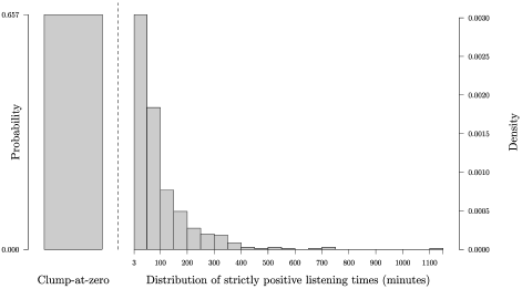
Figure 1: Empirical distribution of the daily listening times to a national radio in an area of the French part of Switzerland during the first semester of 2006. 1382 participants were measured by means of the Radiocontrol system during one day of the period of interest. Zeros represent 65.7% of the data. The distribution of the positive data is extremely skewed with a maximum daily listening time of 1136 minutes. The lowest possible positive listening time is 3 minutes.

We have at our disposal radio audience data of the Swiss measurement system “Radiocontrol” in 2007 [refer to Dähler (2006) for a complete presentation of this measurement system in Switzerland]. As illustrated in Figure 1, the distribution of the daily number of listening minutes $y_{ist}$ for a given radio is extremely skewed, left-truncated and clumped-at-zero. In other words, first, the empirical distribution of the data appears monotonically decreasing. The probability to listen to a radio during a time interval decreases with the time interval length. Second, because of contact validation rules of the Swiss measurement system, the listening times $y_{ist}$ are recorded as zeros if none of the contacts of the participant $i$ to the radio station $s$ last 3–4 minutes or more on day $t$. This means that the smallest observed (recorded as such) listening times are 3–4 minutes. This ensures that the probability to observe false positive contact is negligible over a time interval of 4 or more consecutive minutes. Third, the data contain a high clump-at-zero corresponding to the percentage of people that had no recorded contact with that radio station.

Data with a clump-at-zero and an asymmetric heavy-tail distribution occur in numerous disciplines. Examples are the daily levels of precipitation in an area [Weglarczyk, Strupczewski and Singh (2005)], the yearly amount of car insurance claims per client [Chapados et al. (2002); Christmann (2004)] or the length of overnight stays at hospital per patient [Chen, Jiang and Mao (2007)]. However, no model has been proposed so far for data with a clump-at-zero together with a truncation of small values under a threshold, a model that is necessary to describe, in particular, radio audience data like in our example, but also any other type of data that might, for example for recording reasons, have unreliable measurements at small values of the variable of interest. Hence, the purpose of this paper is to develop a model able to fit truncated heavy-tailed data with excess zeros and to explain, by means of covariates, both the probability associated with a nonzero value and the expectation of positive outcomes. Such a model particularly makes sense in the context of radio audience: The probability of a nonnull value and the expectation of positive outcomes, respectively, correspond to the rating and time spent listening audience indicators. Market shares are a function of these expectations.

Models for data with excess zeros have received much attention in the literature. The most popular ones include the two-part model of Duan et al. (1983) and the zero-inflated count models initiated by Lambert (1992) for continuous data, or the hurdle model of Mullahy (1986) for count data. In Section 2 we describe our model as a natural extension of these models that take into account the left truncation of the outcome variable. To model the positive part of the radio listening times, we propose a zeromodal Pareto-like distribution. Choice has been made for the generalized Pareto distribution because of its ability to fit heavy tails, to be “model invariant” to the choice of the threshold for the left truncation, and because it can be used to only model the tail of the distribution. The resulting model we propose is hence a zero-inflated truncated Pareto (ZITPo) model in which the probability of nonzero outcomes and the mean of the positive outcomes are linked to a set of covariates in a generalized linear model framework. The ZITPo has great fitting flexibility and useful properties as argued in Section 2.5. In Section 3 we investigate by means of simulations the sample properties of the maximum likelihood estimator and inferential procedures. Since ZITPo models are new, it is also important to be able to check the fit of the model and, therefore, we propose in Section 4 a new data analysis tool based on Pareto residuals that is derived in a natural manner from the properties of the ZITPo model. The data from a radio station in a certain area of Switzerland are then fully analyzed in Section 5 by means of the ZITPo which provides an excellent fit to the data and hence good explanatory power for the probability of nonzero outcomes and the mean of the positive outcomes.

2 The ZITPo model

The generalized Pareto distribution, introduced by Pickands (1975), is a limit distribution for the excess over a (large) threshold $\alpha$ for data coming from generalized extreme value distributions, as well as a generalization of the Pareto distribution. The three parameter generalized Pareto distribution has the following cumulative distribution function:

$$F_{Y}(y|\alpha,\tau,\xi)=\cases{\displaystyle 1-\biggl{(}1+\xi\frac{y-\alpha}{\tau}\biggr{)}^{-1/\xi},&\quad\mbox{if } $\xi\neq 0$,\cr\displaystyle 1-\exp\biggl{(}-\frac{y-\alpha}{\tau}\biggr{)},&\quad\mbox{if } $\xi=0$,}$$ (1)

where $\alpha$, $\tau$ and $\xi$ are location, scale and shape parameters, $\alpha\geq 0$ and $\tau>0$. The range of $y$ is $]\alpha,-\frac{\tau}{\xi+\alpha}[$ if $\xi<0$, and $]\alpha,\infty[$ otherwise. The exponential distribution with mean $\tau$ occurs for $\xi=0$. Pareto-like distributions occur for $\xi>0$. The generalized Pareto distribution has been widely used to model rare events in several fields. Applications for environmental extremes are especially numerous (river flow, ozone levels, earthquakes).

For modeling audience radio data, it is also important to be able to link moments or parameters of the generalized Pareto distribution to a set of explanatory variables. The generalized linear models (GLM) framework, introduced by Nelder and Wedderburn (1972), provides a general setting to achieve this aim. GLM are a generalization of the linear regression model in which the assumption of normality of the conditional distribution of the response vector $\mathbf{y}$ given a set of covariates $\mathbf{X}$, $\mathbf{y}|\mathbf{X}$, is relaxed. These models assume that the $i$th unit response, $y_{i}$, follows a distribution belonging to the exponential family, and the expectation of the $i$th response, $y_{i}$, is linked to a set of fixed covariates $\mathbf{x}_{i}$ through an invertible linear predictor function $\nu(\cdot)$, by means of $\mathrm{E}[{Y}_{i}]=\nu^{-1}(\mathbf{x}_{i}\bolds{\beta})$, with $\bolds{\beta}$ a set of regression coefficients. The generalized Pareto distribution falls outside the exponential family framework and, hence, the advantages associated with this framework—like well-known iterative estimation procedures and mathematical properties—are not available. However, extension of the GLM to distributions outside the exponential family is pretty straightforward.

Actually, generalized linear modeling has existed for a long time with responses following extreme value distributions, but not in the traditional scheme that directly relates the response expectation to the explanatory variables through a linear predictor. Indeed, in extreme value analyses, very often the parameters of the response distribution instead of the response expectation are linked to the covariates. Davison and Smith [(1990), page 395] consider that this represents “a more fruitful approach” than the usual one that links the distribution moments to the regressors, as the moments of generalized extreme value distribution do not exist for all values of their parameters. We refer to Coles [(2001), Section 6.4] for a review. In survival analysis, depending on the choice of the hazard function $h(t)$, the survival function $f(t)$ may follow an extreme value distribution. In this context, the hazard function $h(t)=\frac{f(t)}{1-F(t)}$ is then related to the covariates through a linear predictor instead of the response expectation. Such developments may be found in Aitkin and Clayton (1980). As we will see in more details below, for the purpose of modeling radio audience data, it is more sensible to link the expected value of the response to a set of covariates.

Before adapting the generalized Pareto distribution to handle clump-at-zero and left truncation of the positive part of the data, as well as incorporating in the resulting model covariates in order to explain the probability of a zero outcome and the mean of the positive part, we briefly describe models proposed so far for data with excess zeros. The aim is to propose a general formulation from which different models for different situations can be deduced, and, in particular, from which we build our zero-inflated truncated Pareto (ZITPo) model. We then also describe in details the ZITPo model assumptions and discuss some possible extensions.

2.1 Models for nonnegative data with excess zeros

There is a rich literature about adaptation of statistical models to the case of data with excess zeros. We refer to Min and Agresti (2002, 2005) and Ridout, Demétrio and Hinde (1998) for a review. Min and Agresti (2002) compare the advantages and disadvantages of existing approaches and note that the most appealing modeling for continuous data with excess zeros is the two-part model of Duan et al. (1983), and the zero-inflated count models initiated by Lambert (1992) or the hurdle model of Mullahy (1986) in the case of count data with a clump-at-zero. These models are similar. Their key idea is to mix two random variables: A first one, $Y_{1}$, that handles the excess of zeros, and a second one, $Y_{2}$, that models the other part of the data. $Y_{1}$ typically follows a Bernoulli distribution where $P_{Y_{1}}(0)=1-\pi$ denotes the probability to observe a zero outcome. In the hurdle and two-part models (also called conditional models), the probability of the data being equal to zero only depends on $Y_{1}$ and the positive data are all modeled by $Y_{2}$, which may follow a zero-truncated distribution in the case of count data (hurdle model) or a continuous distribution (two-part model). In these cases, $P_{Y_{2}}(0)=0$. In zero-inflated models (also called mixture models), $Y_{2}$ does not follow a zero-truncated distribution. The probability associated to zero thus depends on both $Y_{1}$ and $Y_{2}$.

Let $Y$ be a random variable with probability distribution $P_{Y}$ for the clump-at-zero and the positive part, when the latter is discrete, that is, $Y_{2}$ is discrete, then $P_{Y}$ may be expressed in the following way:

$$P_{Y}(y) = \bigl{[}P_{Y_{1}}(0)+\bigl{(}1-P_{Y_{1}}(0)\bigr{)}P_{Y_{2}}(y)\bigr{]}\iota(y=0)$$

$${}+\bigl{[}\bigl{(}1-P_{Y_{1}}(0)\bigr{)}P_{Y_{2}}(y)\bigr{]}\iota(y>0),$$

where $y=0,1,2,\ldots,$ the indicator function $\iota(\cdot)$ equals one if the condition is true and zero otherwise. Let us refer to a variable as semicontinuous when it has a point mass in zero and a continuous distribution for the positive values [definition of Min and Agresti (2002), page 7]. Then (2.1) may easily be generalized to continuous or semicontinuous $Y_{2}$:

$$f_{Y}(y) = \bigl{[}P_{Y_{1}}(0)+\bigl{(}1-P_{Y_{1}}(0)\bigr{)}P_{Y_{2}}(0)\bigr{]}\delta(y)$$

$${}+\bigl{[}\bigl{(}1-P_{Y_{1}}(0)\bigr{)}f_{Y_{2}}(y)\bigr{]}\Delta_{0}(y),$$

where $\delta(y)$ is a Dirac delta function which equals zero for $y\neq 0$, $\Delta_{0}(y)$ is a step function taking the value of one for $y>0$ and zero otherwise, and $y\in[0,\infty[$. Note that when $P_{Y_{2}}(0)=0$, we have the hurdle or two parts models, while we have zero-inflated models when this is not the case.

The use of the generalized Pareto distribution to model zero-inflated data is not common, one exception being Weglarczyk, Strupczewski and Singh (2005). The authors compare the fitting ability of some semicontinuous distributions to fit hydrological data with excess zeros and consider a Dirac generalized Pareto distribution with density function

$$f_{Y}(y|\pi,\tau,\xi)=(1-\pi)\delta(y)+\frac{\pi}{\tau}\biggl{(}1+\xi\frac{y}{\tau}\biggr{)}^{-1/\xi-1}\Delta_{0}(y),$$ (4)

where $\tau>0$, $\xi\neq 0$, $0\leq(1-\pi)\leq 1$ corresponds to the probability of a zero event. Note that compared to (1), $\alpha=0$. The Dirac generalized Pareto distribution in (4) thus corresponds to a two-part model with $P_{Y_{2}}(0)=0$, in which $f_{Y_{2}}(y)$ is the density function of the generalized Pareto distribution.

In the following sections we propose to extend (2.1) [and (4)] to take into account the possible truncation of small values, as well as to incorporate covariates to explain (a function of) the probability of zero outcomes and the mean distribution of positive outcomes.

2.2 The ZITPo distribution

Let $Y^{*}$ denote the effective (but unknown) daily listening time for a given radio. $Y^{*}$ is to the sum over the day of the dichotomous variables indicating a contact to that radio station minute by minute. The probability and cumulative distribution functions of $Y^{*}$, $f_{Y^{*}}(y^{*})$ and $F_{Y^{*}}(y^{*})$, are semicontinuous with a point mass in zero and a continuous distribution for the positive values. Let $Y$ denote the observed listening times with density function $f_{Y}(y)$. As listening times smaller than a given value $y^{\circ}$ (considered as known) are recorded as zeros, observed zeros are then a mixture between the effective zero listening times and the positive listening times reported as zeros because of the measurement system. Accordingly, $F_{Y}(0)=F_{Y^{*}}(y^{\circ})$.

A semicontinuous version of the zero-inflated count model described in (2.1) is indeed adequate to model the double origins of the zeros in the clump-at-zero and the positive values of the observed listening times. Let us assume that the unknown and true proportion of zero listening times is $1-\pi$, with $0\leq\pi\leq 1$, and that the effective positive listening times follow a two parameter generalized Pareto distribution (with $\alpha=0$), $Y^{*}|(Y^{*}>0)\sim\mathrm{GPD}(\tau,\xi)$. Then, in (2.1), $P_{Y_{1}}(0)=1-\pi$ corresponds to the effective proportion of nonlisteners, and $P_{Y_{2}}(0)=F_{(Y^{*}|Y^{*}>0)}(y^{\circ})$ corresponds to the part of the two parameter generalized Pareto distribution that cannot be observed because of the measurement system limitations. The density functions of the effective listening times $Y^{*}$ and of the observed listening times $Y$ are

$$f_{Y^{*}}(y^{*}|\pi,\tau,\xi) = [1-\pi]\delta(y^{*})+\biggl{[}\frac{\pi}{\tau}\biggl{(}1+\xi\frac{y^{*}}{\tau}\biggr{)}^{-1/\xi-1}\biggr{]}\Delta_{0}(y^{*}),$$ (5)

$$f_{Y}(y|\pi,\tau,\xi) = \bigl{[}(1-\pi)+\pi F_{(Y^{*}|Y^{*}>0)}(y^{\circ})\bigr{]}\delta(y)$$

$${}+\bigl{[}\pi f_{(Y^{*}|Y^{*}>0)}(y)\bigr{]}\Delta_{y^{\circ}}(y)$$

$$= \biggl{[}1-\pi\biggl{(}1+\xi\frac{y^{\circ}}{\tau}\biggr{)}^{-1/\xi}\biggr{]}\delta(y)$$

$${}+\biggl{[}\frac{\pi}{\tau}\biggl{(}1+\xi\frac{y}{\tau}\biggr{)}^{-1/\xi-1}\biggr{]}\Delta_{y^{\circ}}(y),$$

where $0\leq\pi\leq 1$, $\tau>0$, $\xi\neq 0$ and $y^{\circ}\geq 0$. For $y^{\circ}=0$, (2.2) reduces to the Dirac generalized Pareto described in (4). Finally, note that if the observed listening times distribution in (2.2) has the disadvantage of being a mixture distribution which makes it more complex to fit, its underlying distribution in (5) takes the advantages of the orthogonal parameterization of the hurdle and two-part models and is thus easier to interpret [for a discussion on the orthogonal parameterization see, e.g., Welsh et al. (1996)]. Indeed, the zeros depend on $\pi$, while the positive outcomes rely on the generalized Pareto parameters, $\tau$ and $\xi$.

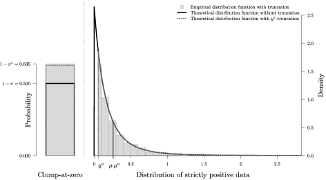
Figure 2: Empirical distribution function of a data set simulated from a ZITPo model with parameters $\pi=0.5$, $\mu=\xi=0.25$ and $y^{\circ}=F^{-1}_{(Y^{*}|Y^{*}>0)}(0.25)$. The theoretical truncated and untruncated density functions are superimposed to the plot with dashed gray and black lines. The value of the expectations of the positive values of the truncated and untruncated distributions, $\mu^{\circ}$ and $\mu$, are indicated on the x-axis. On the discrete part of the plot, the surfaces within the dashed gray and black boxes correspond to the theoretical probabilities to observe zeros when there is (dashed gray) and when there is no (black) left truncation of the positive part of the data. Those probabilities respectively equal $1-\pi$ and $1-\pi^{\circ}=(1-\pi)+\pi F^{-1}_{(Y^{*}|Y^{*}>0)}(y^{\circ})$.

Figure 2 shows the distribution of a data set simulated from a ZITPo distribution. The theoretical untruncated and truncated distribution functions, respectively corresponding to (5) and (2.2), are respectively superimposed to the plot in black and dashed gray lines. On the discrete part of the plot, the surfaces within the dashed gray and black boxes correspond to the theoretical probabilities to observe zeros when there is (dashed gray) and when there is no (black) left truncation of the positive part of the data. Those probabilities respectively equal $1-\pi$ and $1-\pi^{\circ}=(1-\pi)+\pi F^{-1}_{(Y^{*}|Y^{*}>0)}(y^{\circ})$. On the continuous part of the plot, the expectations of the truncated ($\mu^{\circ}$) and untruncated ($\mu$) distributions are indicated. It is then clear that the expected value for the true listening time $Y^{*}$, $\mu$, is different from the expected value of the truncated distribution, $\mu^{\circ}$. For the audience data, one quantity of interest is $\mu$ for the untruncated distribution.

2.3 Covariates modeling in ZITPo distribution

Adaptation of the GLM to models for data with excess zeros is very intuitive. The expectations of the distributions of $Y_{1}$ and $Y_{2}$ in (2.1) and (2.1) are linked to the covariates through adapted link functions. The logit link is often chosen to relate the expectation of $Y_{1}$, corresponding to the probability to observe positive values, to the covariates. The log link makes sense to connect the expectation of $Y_{2}$, corresponding to the mean of the positive data, to the covariates, as this last is necessarily positive. For the $i$th observation, we then have

$$\pi_{i} = \mathrm{P}(Y^{*}_{i}>0)=\nu_{1}^{-1}(\mathbf{x}_{i1}^{T}\bolds{\beta}_{1})=\frac{\exp(\mathbf{x}_{i1}^{T}\bolds{\beta}_{1})}{1+\exp(\mathbf{x}_{i1}^{T}\bolds{\beta}_{1})},$$ (7)

$$\mu_{i} = \mathrm{E}[Y^{*}_{i}|Y^{*}_{i}>0]=\nu_{2}^{-1}(\mathbf{x}_{i2}^{T}\bolds{\beta}_{2})=\exp(\mathbf{x}_{i2}^{T}\bolds{\beta}_{2}),$$ (8)

where $\nu_{1}^{-1}(\cdot)$ and $\nu_{2}^{-1}(\cdot)$ are the inverse of the linear predictor functions linking the expectations of $Y_{1}$ and $Y_{2}$ in (2.1) and (2.1) to the covariates, $\mathbf{x}_{i1}$ and $\mathbf{x}_{i2}$ are the covariates of the $i$th observation that may contain the same predictors, and $\bolds{\beta}_{1}$ and $\bolds{\beta}_{2}$ are the corresponding parameters. Because of the orthogonal parameterization of the underlying model in (5), if we use in (7) and (8) two different and uncorrelated sets of covariates, $\mathbf{X}_{1}$ and $\mathbf{X}_{2}$, we then assume that the processes that explain the probability to observe a positive outcome and the expectation of a positive outcome are independent. If part of the covariates of $\mathbf{X}_{1}$ are present in (or correlated to) $\mathbf{X}_{2}$, $\pi_{i}$ and $\mu_{i}$ will possibly be linked. No assumption is done about the form of the relationship between these quantities.

Inclusion of covariates in (4) requires that we express the distribution $f_{Y}(y)$ in terms of the expectation of the positive values of the data. Let $(Y^{*}|Y^{*}>0)\sim\mathrm{GPD}(\tau,\xi)$. Then

$$\mu=\mathrm{E}[Y^{*}|Y^{*}>0]=\frac{\tau}{1-\xi}\qquad\mbox{for }1-\xi>0.$$

The first moment of the generalized Pareto distribution, $\mu$, thus exists for values of $\xi$ lower than one. Substituting $\tau$ by $\mu(1-\xi)$ in (2.2) gives

$$f_{Y}(y|\pi,\mu,\xi) = \biggl{[}1-\pi\biggl{(}1+\biggl{(}\frac{\xi}{1-\xi}\biggr{)}\frac{y^{\circ}}{\mu}\biggr{)}^{-1/\xi}\biggr{]}\delta(y)$$

$${}+\biggl{[}\frac{\pi}{\mu(1-\xi)}\biggl{(}1+\biggl{(}\frac{\xi}{1-\xi}\biggr{)}\frac{y}{\mu}\biggr{)}^{-1/\xi-1}\biggr{]}\Delta_{y^{\circ}}(y),$$

with $0\leq\pi\leq 1$, $\mu>0$, $\xi\neq 0$ and $\xi<1$, $y^{\circ}\geq 0$. The inclusion of the covariates as described in (7) and (8) is now straightforward. For the $i$th observation, we have

$$f_{Y_{i}}(y_{i}|\mathbf{x}_{i1},\mathbf{x}_{i2},\bolds{\beta}_{1},\bolds{\beta}_{2},\xi)$$

$$\qquad=\,\biggr{[}1-\frac{\exp(\mathbf{x}_{i1}^{T}\bolds{\beta}_{1})}{1+\exp(\mathbf{x}_{i1}^{T}\bolds{\beta}_{1})}\biggl{(}1+\biggl{(}\frac{\xi}{1-\xi}\biggr{)}\frac{y^{\circ}}{\exp(\mathbf{x}_{i2}^{T}\bolds{\beta}_{2})}\biggr{)}^{-1/\xi}\biggr{]}\delta(y)$$

(10)

$$\qquad\quad{}+\biggl{[}\frac{\exp(\mathbf{x}_{i1}^{T}\bolds{\beta}_{1})}{1+\exp(\mathbf{x}_{i1}^{T}\bolds{\beta}_{1})}\frac{1}{\exp(\mathbf{x}_{i2}^{T}\bolds{\beta}_{2})(1-\xi)}$$

$$\qquad\qquad\hskip 5.0pt{}\times\biggl{(}1+\biggl{(}\frac{\xi}{1-\xi}\biggr{)}\frac{y_{i}}{\exp(\mathbf{x}_{i2}^{T}\bolds{\beta}_{2})}\biggr{)}^{-1/\xi-1}\biggr{]}\Delta_{y^{\circ}}(y).$$

2.4 Assumptions of ZITPo models

The form of the ZITPo model implies a number of assumptions on the distribution of the positive values:

First, the unobserved positive listening times belonging to the range $]0,y^{\circ}[$ correspond to the nonobserved part of a left-truncated generalized Pareto distribution. As the generalized Pareto density function is zero modal and monotonically decreasing, this assumption implies that, conditionally on the covariates, the probability of positive listening times in the interval $]0,y^{\circ}[$ is higher than in any other interval of the same size. As zapping through radio is frequent, we believe that this assumption is realistic.

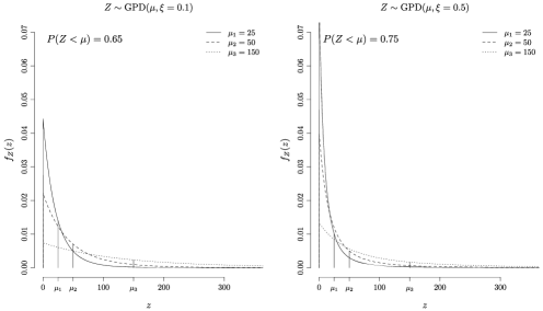
Figure 3: Examples of two parameter generalized Pareto distributions. In both plots, three distribution functions sharing the same $\xi$-value are proposed. Their respective expectations are $\mu_{1}=25,\mu_{2}=50$ and $\mu_{3}=100$. The probability to observe data below the expectation is indicated above.

Second, the expectation $\mu_{i}$ always corresponds to the quantile $1-(1-\xi)^{1/\xi}$ of a $\mathrm{GPD}(\mu_{i},\xi)$. Indeed, conditionally on the covariates, as the real positive listening times follow generalized Pareto distributions having different expectations $\mu_{i}$ but sharing the same $\xi$-value, $Y_{i}^{*}|(Y_{i}^{*}>0)\sim\mathrm{GPD}(\mu_{i},\xi)$, we can observe that

$$F_{(Y_{i}^{*}|Y_{i}^{*}>0)}(\mu_{i})=1-\biggl{(}1+\xi\frac{\mu_{i}}{\mu_{i}(1-\xi)}\biggr{)}^{-1/\xi}=1-(1-\xi)^{1/\xi}.$$ (11)

Figure 3 shows examples of two parameter generalized Pareto density functions sharing the same $\xi$-value (within the same graph) but having different expectations. For the same $\xi$-value, the density functions show a great variety of forms and thus a high ability to model different data sets with more or less heavy tails.

Third, because of the reparametrization of the generalized Pareto density formulated in (2.3), the shape parameter is restricted to values lower than one. This does not seem problematic in regard to (11). Indeed, for $\xi>0.95$, $\mu$ corresponds to quantiles of the distribution higher than 0.95. We do not expect cases in which the theoretical mean belongs to the last 5% of the distribution at least with radio listening data.

Fourth, because of the logit link used in (7), the probability to tune into a given radio station conditional on covariates never equals zero or one as $\exp(\mathbf{x}_{i1}^{T}\bolds{\beta}_{1})>0$. We do believe that it is reasonable to state that $0<\pi_{i}<1$ in radio audience data:

• As radio stations broadcast almost everywhere (airports, supermarkets, petrol stations$,\ldots$), it seems reasonable to state that the probability of contact of anybody is greater than zero.

• As radio stations do not broadcast everywhere, it also seems reasonable to state that even the biggest fan of a specific radio station can, for example, be outside the broadcasting range at some specific times.

2.5 Properties and extensions of ZITPo models

Even if there are some restrictions in the use of ZITPo models, the two-part form of the density described in (2.3) as well as properties of the generalized Pareto distribution offer to ZITPo models additional abilities to fit and analyze a variety of data sets, in particular, our radio audience data in Switzerland:

First, one interesting property of ZITPo models is that $y^{\circ}$ may be chosen such that the observed data lower than $y^{\circ}$ integrate the most part of the false zero and false positive observations if the data are not completely reliable in the neighborhood of the truncation boundary. If all observed positive data inferior to $y^{\circ}$ are coded as zeros in order to belong to the clump-at-zero in (2.2), the model will estimate the parameters of $f_{Y^{*}}(y^{*}|\pi,\tau,\xi)$ without being affected by the errors of the measurement system occurring on $[0,y^{\circ}[$.

Second, the stability with respect to excess over threshold operations of the generalized Pareto distribution [see, e.g., Castillo and Hadi (1997), page 1610, or Coles (2001), page 79] and the shifting property of distribution of the location family allow to easily determine the distribution of the data over a threshold $y^{\bullet}$. Let $Y_{i}^{*+}=(Y_{i}^{*}|Y_{i}^{*}>0)$ denote the positive values of the model, with $Y_{i}^{*+}\sim\mathrm{GPD}(\tau_{i},\xi)$ with $\tau_{i}=\mu_{i}(1-\xi)$. Then we have that

$$f_{(Y_{i}^{*+}|Y_{i}^{*+}>y^{\bullet})}(y_{i}^{*+}|\tau_{i},\xi)=\frac{1}{\tau_{i}-\xi y^{\bullet}}\biggl{(}1+\xi\frac{y_{i}^{*+}-y^{\bullet}}{\tau_{i}-\xi y^{\bullet}}\biggr{)}^{-1/\xi-1}.$$ (12)

This is of particular interest for radio station managers and advertisers, as important radio listeners represent the core of their audience. The distribution of the listening time over a threshold thus follows a three parameter generalized Pareto distribution of parameters $\alpha^{\bullet}=y^{\bullet}$, $\tau_{i}^{\bullet}=\tau_{i}-\xi y^{\bullet}$ and $\xi^{\bullet}=\xi$. The corresponding expected listening time over a threshold of $y^{\bullet}$ minutes, $\mu^{\bullet}_{i}$, is then given by

$$\mu^{\bullet}_{i}=\mathrm{E}[Y^{*+}|Y^{*+}>y^{\bullet}]=\frac{\tau_{i}^{\bullet}}{1-\xi}+y^{\bullet}=\mu_{i}+\frac{\xi y^{\bullet}}{1-\xi}+y^{\bullet},$$ (13)

where $\mu_{i}=\mu$ in simple models without covariates and $\mu_{i}=\exp(\mathbf{x}_{i2}^{T}\bolds{\beta}_{2})$ in models incorporating covariates. The expectation of the positive data over a threshold (i.e., the expectation of the data on $]y^{\bullet},\infty[$) thus simply corresponds to a linear shift of the expectation of the positive data on $]0,\infty[$. There is therefore no need to change the ZITPo model when one is interested in $\mu^{\bullet}_{i}$ or, in other words, the effect of the covariates on $\mu^{\bullet}_{i}$ is the same as on $\mu_{i}$.

Third, the ZITPo model can easily be extended to the three parameter generalized Pareto distribution by introducing a shift parameter $y^{\bullet}\leq y^{\circ}$ corresponding to $\alpha$ in (1). In (2.3) and (2.3) we have that $y^{\bullet}=0$. Adding the shift parameter makes sense if information below $y^{\bullet}$ is not of direct interest, like if nonlisteners and listeners that only zap through a given radio are considered alike for the radio broadcaster. The resulting model which extends (2.3) [and consequently (2.3)] would allow to model the probability to get an outcome lower than a given positive value $y^{\bullet}$ as well as the expectation of the data over $y^{\bullet}$, with positive outcomes observed above $y^{\circ}$. In this case, all data lower than $y^{\bullet}$ would be treated as “zeros” in order to be part of the clump-at-zero. The density functions of the observed listening times $Y$ would then be (for an observation $y_{i}$)

$$f_{Y}(y_{i}|\pi^{\bullet}_{i},\mu^{\bullet}_{i},\xi^{\bullet}) = \biggl{[}1-\pi^{\bullet}_{i}\biggl{(}1+\biggl{(}\frac{\xi}{1-\xi}\biggr{)}\biggl{(}\frac{y^{\circ}-y^{\bullet}}{\mu^{\bullet}_{i}-y^{\bullet}}\biggr{)}\biggr{)}^{-1/\xi}\biggr{]}\delta(y_{i})$$

$${}+\biggl{[}\frac{\pi^{\bullet}_{i}}{(\mu^{\bullet}_{i}-y^{\bullet})(1-\xi)}$$

$$\quad\hskip 5.0pt{}\times\biggl{(}1+\biggl{(}\frac{\xi}{1-\xi}\biggr{)}\biggl{(}\frac{y_{i}-y^{\bullet}}{\mu^{\bullet}_{i}-y^{\bullet}}\biggr{)}\biggr{)}^{-1/\xi-1}\biggr{]}\Delta_{y^{\circ}}(y_{i}).$$

The parameters $\pi^{\bullet}_{i}$ and $\mu^{\bullet}_{i}$ can possibly be linked to a set of covariates as is done in (2.3). If there is no $y^{\circ}$-truncation and if the data on $]y^{\bullet},y^{\circ}[$ are reliable, $y^{\circ}=y^{\bullet}$ and (2.5) is reduced to a two-part model since the first part of the right-hand side of (2.5) reduces to $(1-\pi^{\bullet}_{i})\delta(y_{i})$. This extension is particularly useful when the interest only lies on the tail distribution of the positive outcomes. Indeed, in that case $\pi^{\bullet}$ is a nuisance parameter and the generalized Pareto distributional assumption on $]0,y^{\bullet}[$ is no more necessary. For the model to fit the data (observed above $y^{\circ}$), one only needs the assumption that the generalized Pareto distribution holds above $y^{\bullet}$, with a mean that possibly depends on a set of covariates and constant $\xi$. This might be an interesting setting, for example, in finance when seeking to explain the value-at-risk of financial instruments. In these cases, however, the choice of $y^{\bullet}$ might become an important issue and criteria based on mean squared errors [see, e.g., Hill (1975); Hall and Welsh (1985); Beirlant, Vynckier and Teugels (1996)] or prediction errors [Dupuis and Victoria-Feser (2006)] could, in principle, be extended to the ZITPo. In what follows, we will, however, focus on models with $y^{\bullet}=0$.

3 Estimation and inference

Fitting methods for the generalized Pareto distribution in (1) (i.e., without a clump-at-zero) has been of great interest in the literature. Castillo and Hadi (1997) and Singh and Ahmad (2004) propose a comparative evaluation of the most used classical estimators for the two and three parameter distributions. Robust estimators have also been developed [Dupuis and Tsao (1998); Peng and Welsh (2001); Juárez and Schucany (2004)]. We propose here to use the maximum likelihood estimator (MLE).

The log-likelihood function of the ZITPo model described in (2.3) is

$$l(\bolds{\beta}_{1},\bolds{\beta}_{2},\xi|\mathbf{y},y^{\circ},\mathbf{X}_{1},\mathbf{X}_{2})$$

$$\qquad=\Biggl{\{}\sum_{i=1}^{n}\iota(y_{i}=0)\log\biggl{[}1-\frac{\exp(\mathbf{x}_{i1}^{T}\bolds{\beta}_{1})}{1+\exp(\mathbf{x}_{i1}^{T}\bolds{\beta}_{1})}$$

$$\hskip 132.0pt{}\times\biggl{(}1+\biggl{(}\frac{\xi}{1-\xi}\biggr{)}\biggl{(}\frac{y^{\circ}}{\exp(\mathbf{x}_{i2}^{T}\bolds{\beta}_{2})}\biggr{)}\biggr{)}^{-1/\xi}\biggr{]}\Biggr{\}}$$ (15)

$$\qquad\quad{}+\Biggl{\{}\sum_{i=1}^{n}\Delta_{y^{\circ}}(y)\biggl{[}\mathbf{x}_{i1}^{T}\bolds{\beta}_{1}-\mathbf{x}_{i2}^{T}\bolds{\beta}_{2}-\log\biggl{(}\frac{(1-\xi)^{-1}}{1+\exp(1+\mathbf{x}_{i1}^{T}\bolds{\beta}_{1})}\biggr{)}\biggr{]}\Biggr{\}}$$

$$\qquad\quad{}+\Biggl{\{}\sum_{i=1}^{n}\Delta_{y^{\circ}}(y)\biggl{(}-\frac{1}{\xi}-1\biggr{)}\log\biggl{(}1+\biggl{(}\frac{\xi}{1-\xi}\biggr{)}\biggl{(}\frac{y_{i}}{\exp(\mathbf{x}_{i2}^{T}\bolds{\beta}_{2})}\biggr{)}\biggr{)}\Biggr{\}}.$$

Maximization of this expression is achieved using the quasi-Newton method with a numerically computed gradient matrix. Convergence is obtained rapidly for most of the cases we have tried, even with models embedding many covariates. The use of slightly different starting values did always provide a solution to the unusual cases in which we met convergence problems. The program is implemented in R functions available in Couturier and Victoria-Feser (2010).

In order to check the finite sample properties of the MLE for the ZITPo model, we perform a simulation study of models incorporating covariates as in (2.3). The MLE is computed on samples with three different sample sizes of respectively 500, 1000 and 2000 observations, simulated with two different values for the shape parameter, $\xi=0.25$ and $\xi=0.5$. The sampling distribution of the MLE are presented by means of boxplots on 2500 simulated data sets. Horizontal gray lines indicate the position of the true parameter values. The coverage levels of 95%-confidence intervals of the form $[\hat{\theta}-\Phi^{-1}(0.975)\hat{\sigma}_{\hat{\theta}},\hat{\theta}+\Phi^{-1}(0.975)\hat{\sigma}_{\hat{\theta}}]$, where $\Phi$ is the probability function of the standard normal distribution and where $\hat{\sigma}_{\hat{\theta}}$ are obtained from the inverse of the estimated Hessian matrix, are also indicated.

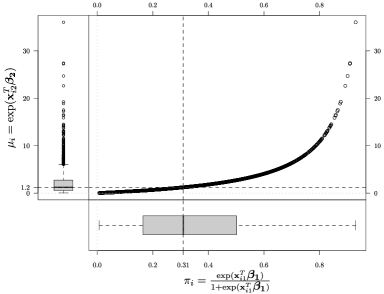
Figure 4: Distribution of the probabilities of positive outcomes, $\pi_{i}$, and of the expectations of positives values, $\mu_{i}$, used to simulate ZITPo realizations.

The data are simulated from a ZITPo distribution with parameters

$$\pi_{i}=\frac{\exp(\mathbf{x}_{i1}^{T}\bolds{\beta}_{1})}{1+\exp(\mathbf{x}_{i1}^{T}\bolds{\beta}_{1})}\quad\mbox{and}\quad\mu_{i}=\exp(\mathbf{x}_{i2}^{T}\bolds{\beta}_{2}).$$

For the covariates, the same $\mathbf{X}$ matrix is used in both parts of the model. The first column of $\mathbf{X}$ is a column vector of $1$ corresponding to the constant. The other columns of $\mathbf{X}$ were constructed with random values of respectively a normal, a Poisson, two binomials and an exponential distribution, with corresponding regression parameters $\bolds{\beta}_{1}=[1,1,-0.5,0.5,0.25,0.25]^{T}$ and $\bolds{\beta}_{2}=[2,1,0.5,0.5,0.25,0.25]^{T}.$ The values of the $\bolds{\beta}_{1}$ and $\bolds{\beta}_{2}$ were chosen in order to obtain asymmetrical distributions for the probabilities of positive outcomes, $\pi_{i}$, and for the expectations of positives values, $\mu_{i}$, as well as a positive relationship between these quantities. Figure 4 shows their respective distributions as well as the chosen relationship between $\pi_{i}$ and $\mu_{i}$. With a median of 0.3, the probabilities of positive outcomes, $\pi_{i}$, are rather low. The expectations of the positives values, $\mu_{i}$, have a very asymmetrical distribution. The cutting value $y^{\circ}=0.125$ is a fixed value independent of $i$ and which approximately corresponds to the quantile 0.1 of the positive simulated data. The form of the dependance between $\pi_{i}$ and $\mu_{i}$ is nonlinear. The choice of the parameter values $\pi_{i},\mu_{i}$ and $y^{\circ}$ thus corresponds to an extreme choice to test the performance of the MLE in nontrivial situations.

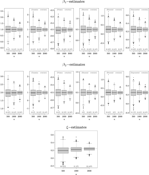
Figure 5: Boxplots of the MLE of $\bolds{\beta}_{1}$ (upper plots), $\bolds{\beta}_{2}$ (centered plots) and $\xi$ (bottom plot) computed over 2500 datasets simulated from a ZITPo distribution with parameters $\bolds{\beta}_{1}=[1,1,-0.5,0.5,0.25,0.25]^{T}$, $\bolds{\beta}_{2}=[2,1,0.5,0.5,0.25,0.25]^{T}$ and $\xi=0.25$. $y^{\circ}=0.125$ is a fixed value which approximately corresponds to the quantile 0.1 of the positive simulated data. Analyses were performed for samples of sizes 500, 1000 and 2000. The horizontal gray lines indicate the position of the true parameter values. The coverage levels of confidence intervals of the form $[\hat{\theta}-\Phi^{-1}(0.975)\hat{\sigma}_{\hat{\theta}},\hat{\theta}+\Phi^{-1}(0.975)\hat{\sigma}_{\hat{\theta}}]$, where $\Phi$ is the probability function of the standard normal distribution, are also indicated.

The bottom plot of Figure 5 shows the sampling distribution of the MLE of the shape parameter $\xi$. The boxplots of the parameters estimates of $\xi$ show a small underestimation of the parameter value even when the number of positive data is around 650 observations which correspond to 30% of the maximum sample size of this analysis. Estimation of the shape parameter is known to be problematic even with large sample sizes and regardless of the estimating method [Hosking and Wallis (1987)]. Our simulations tend to show that the bias of the shape parameter both depends on the number of observations $n$ and on the number of covariates $p$, a situation similar to the MLE of the parameter $\sigma$ in multiple regression analyses. This also confirms the findings of Chavez-Demoulin and Davison [(2005), page 212] for $\xi$ in their adaptation of generalized additive models to the generalized Pareto distribution.

The upper and centered plots of Figure 5 present the sampling distributions of the MLE of $\bolds{\beta}_{1}$ and $\bolds{\beta}_{2}$. Regardless of the sample size, all boxplots are well centered around the true value of the parameters and the coverage levels of the corresponding confidence intervals are close to the $95\%$ nominal value. As $\bolds{\beta}_{2}$ and the $\xi$ are essentially estimated over the positive part of the data which represent the 30% of the 500, 1000 and 2000 observations of our study, our results appear very satisfactory. Similar results were obtained in simulations with $\xi=0.5$.

4 Model validation

Residual analyses in the context of models for data with excess zeros as described in (2.1) and (2.1) may be split in two parts: A first one focusing on the distribution that distinguishes the zeros from the positive outcomes, and a second one considering the distribution of the positive values. In models with covariates, the residuals of the part distinguishing the zeros correspond to residuals of logistic regressions. As this topic is already well covered in the literature [we refer to Collett (2003) for a complete overview], the following subsections focus on the residuals of the positive part of the model. We propose a residual type for truncated and untruncated generalized Pareto models. Section 5 presents one use of this new residual type.

Let $Y_{i}^{*+}=(Y_{i}^{*}|Y_{i}^{*}>0)$ denote the positive values of the model and let $Y_{i}^{+}=(Y_{i}|Y_{i}>y^{\circ})$ be the observed truncated positive values. As $(Y_{i}^{*+}-y^{\circ}|Y_{i}^{*+}>y^{\circ})=(Y_{i}^{+}-y^{\circ})$ and follows a $\mathrm{GPD}(\mu_{i}+\frac{\xi y^{\circ}}{1-\xi},\xi)$, let us define the $i$th residual, $\varepsilon_{i}$, in the following way:

$$\varepsilon_{i}=h(Y_{i}^{+}-y^{\circ})=\frac{Y_{i}^{+}-y^{\circ}}{\mathrm{E}[Y_{i}^{+}-y^{\circ}]}=\frac{Y_{i}^{+}-y^{\circ}}{\mu_{i}+\xi y^{\circ}/(1-\xi)}.$$ (16)

The residuals distribution, $f_{\varepsilon_{i}}(\varepsilon_{i})$, may then easily be derived and is given by

$$f_{\varepsilon_{i}}(\varepsilon_{i}) = f_{(Y^{+}_{i}-y^{\circ})}(h^{-1}(\varepsilon_{i}))\biggl{|}\frac{\partial}{\partial\varepsilon_{i}}h^{-1}(\varepsilon_{i})\biggr{|}$$

$$= \frac{1}{1-\xi}\biggl{(}1+\frac{\xi}{1-\xi}\varepsilon_{i}\biggr{)}^{-1/\xi-1}.$$

Thus, $f_{\varepsilon_{i}}(\varepsilon_{i})\sim\mathrm{GPD}(\mu=1,\xi)$. The residuals theoretically (i.e., if the ZITPo model holds) follow a generalized Pareto distribution of parameters $\mu=1$ and $\xi$. This result holds also when $y^{\circ}=0$. Note that this result is a finite sample result, a pretty rare situation in GLM. A very powerful finite sample model validation procedure thus consists in comparing the distribution of the estimated residuals to their estimated theoretical distribution. The former are obtained by substituting in (16) the parameters by their estimated values, that is,

$$\hat{\varepsilon}_{i}=\frac{Y_{i}^{+}-y^{\circ}}{\hat{\mu}_{i}+\hat{\xi}y^{\circ}/(1-\hat{\xi})}\sim\mathrm{GPD}(\mu=1,\hat{\xi}).$$

QQ-plots should approximately display a straight line when the model adequately fits the data.

Finally, the result in (4) offers a fast method to generate random realizations from truncated or untruncated generalized Pareto models. Indeed, let $u$ be a random realization of a $\mathrm{Uniform(0,1)}$ and let $\mu$ be the vector of expectations of the generalized Pareto distribution. Then, inverting (16) and (4) allows to generate $y$, a random variate of a $y^{\circ}$-truncated $\mathrm{GPD}(\mu,\xi)$, in the following way:

$$y=\biggl{[}(u^{-\xi}-1)\frac{1-\xi}{\xi}\biggr{]}\biggl{(}\mu+\frac{\xi y^{\circ}}{1-\xi}\biggr{)}+y^{\circ}.$$

5 Applications to radio audience data

The ZITPo model is applied to the audience data of the local radio station “116” in its broadcasting area during the weekdays of the second semester of 2007. The data set is available in Couturier and Victoria-Feser (2010). The left upper plot of Figure 7 presents the distribution of the daily listening times of 2155 participants measured during one day of this period. The clump-at-zero represents 63% of the data.

The audience indicators of rating and time spent listening are explained by a set of categorical variables including the age in 5 classes ($[15,25[,$ $[25,35[,$ $[35,45[,$ $[45,60[,$ $[60,120[$), the education level in 3 classes (low, mid, high), the gender, the time in month and the different zones of the broadcast area. The contrasts used to create the $k-1$ dummy variables from a $k$-classes categorical variable are of type “treatment” for the variables age, gender and education with base “15 to 25 years old men with low education level,” and of type “Sum” for the geographical zones and the months. The model includes interaction between age and gender. Other interactions—like between education and age—appeared nonsignificant and did not improve the log-likelihood or the residual distribution.

To protect the parameter estimates of the possible influence of the false positive and false zeros observations belonging to the interval $[0,5[$, we choose $y^{\circ}=4.95$. Consequently, we coded the 19 observations belonging to the interval $[3,5[$ in Figure 7 as zeros and let the ZITPo model adequately separate the true from the false zeros as described in the first part of (2.3).

Table 1: $\bolds{\beta}_{1}$ and $\bolds{\beta}_{2}$ estimated parameters and corresponding standard deviations of the ZITPo model applied to the listening times to radio station “116.” The $p$-values are for (asymptotic) significance testing of $\bolds{\beta}_{1}$ and $\bolds{\beta}_{2}$. Low $p$-values are magnified in the columns “Sig.” by means of (***), (**), (*), ($\cdot$) respectively corresponding to significant tests at the levels of 0.001, 0.01, 0.05 and 0.1

	Rating				Average listening time
	$\bolds{\hat{\beta}}_{\mathbf{1}}$	SE	p-value	Sig.	$\bolds{\hat{\beta}}_{\mathbf{1}}$	SE	p-value	Sig.
(Intercept)	$-$1.95	0.32	$<$0.001	***	$-$4.08	0.33	$<$0.001	***
$[$25–35$[$	$-$0.40	0.39	$<$0.309		$-$0.16	0.39	$<$0.680
$[$35–45$[$	$-$0.94	0.36	$<$0.008	**	$-$0.20	0.35	$<$0.568
$[$45–60$[$	$-$1.57	0.34	$<$0.001	***	$-$0.40	0.34	$<$0.235
$[$60–120$[$	$-$2.22	0.35	$<$0.001	***	$-$0.76	0.34	$<$0.026	*
Women	$-$0.25	0.49	$<$0.608		$-$0.73	0.49	$<$0.133
Educ. middle	$-$0.18	0.16	$<$0.255		$-$0.01	0.13	$<$0.933
Educ. high	$-$0.36	0.12	$<$0.002	**	$-$0.15	0.09	$<$0.103
July	$-$0.15	0.12	$<$0.216		$-$0.06	0.10	$<$0.516
August	$-$0.11	0.11	$<$0.346		$-$0.04	0.09	$<$0.695
September	$-$0.14	0.11	$<$0.225		$-$0.07	0.09	$<$0.393
October	$-$0.18	0.11	$<$0.085	$\cdot$	$-$0.01	0.08	$<$0.948
November	$-$0.00	0.11	$<$0.973		$-$0.04	0.09	$<$0.654
Zone 2	$-$0.26	0.05	$<$0.001	***	$-$0.08	0.04	$<$0.049	*
Women $+[$25–35$[$	$-$0.02	0.58	$<$0.970		$-$1.26	0.57	$<$0.028	*
Women $+[$35–45$[$	$-$0.18	0.54	$<$0.737		$-$0.71	0.53	$<$0.180
Women $+[$45–60$[$	$-$0.03	0.52	$<$0.961		$-$0.90	0.51	$<$0.079	$\cdot$
Women $+[$60–120$[$	$-$0.39	0.52	$<$0.455		$-$1.11	0.50	$<$0.027	*

The $\bolds{\beta}_{1}$ and $\bolds{\beta}_{2}$ estimated values as well as their standard deviations are reported in Table 1. The $p$-values corresponding to the (asymptotic) significance tests for $\bolds{\beta}_{1}$ and $\bolds{\beta}_{2}$, that is, $2\Phi^{-1}(-|\hat{\beta}/\hat{\sigma}_{\hat{\beta}}|)$, are also indicated. According to the chosen contrasts, the estimated intercepts $\beta_{10}$ and $\beta_{20}$ are related to the estimated rating and time spent listening of 15 to 25-year-old men with a low education level in the broadcast area of interest during the second semester of 2007 through, respectively,

$$\frac{\exp(\hat{\beta}_{10})}{1+\exp(\hat{\beta}_{10})}\cong 0.12\quad\mbox{and}\quad\exp(\hat{\beta}_{20})\cong 59.$$

15–25-year-old men living in the broadcast area of interest and having a low education level have thus a probability of contact to radio station “116” of 12% and an average contact length of about 59 minutes during the second semester of 2007. The estimated distribution of the effective (untruncated) positive times of the individuals of this focus group is thus

$$Y_{i}^{*}|(Y_{i}^{*}>0)\sim\mathrm{GPD}(59,\hat{\xi}\cong 0.082).$$

Thus, under the model, $F^{-1}_{(Y^{*}|Y^{*}>0)}(3|59,\hat{\xi})\cong 0.05$ and $F^{-1}_{(Y^{*}|Y^{*}>0)}(y^{\circ}|59,\hat{\xi})\cong 0.09$ respectively represent for this focus group the estimation of the part of effective positive data that is coded as zero by the Swiss measurement system and the estimation of the part of the effective positive data that was supposed truncated and coded as zero for the estimation. The average ratings and time spent listening of other focus groups—like women with a high education level—are then shifts of 12% and 59 minutes. Figure 6, for example, presents the estimated (untruncated) listening times distributions of men with low eduction level conditional to 5 age classes. The probability to tune into this radio station strongly depends on the age class. The expected listening times are more or less the same for 15–45-year-old men and increase then for the two oldest age classes.

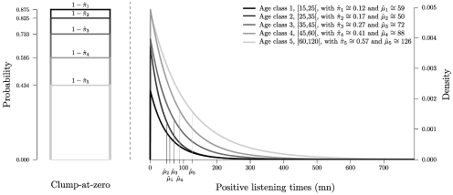
Figure 6: Estimated (untruncated) listening times distributions of men with low eduction level conditional to 5 age classes. The probability to tune into this radio station strongly depends on the age class. The expected listening times are more or less the same except for the oldest age class.

In order to test the significance of each factor (e.g., age), we use the likelihood ratio test to compare nested models. Let $\bolds{\beta}=[\bolds{\beta}^{T}_{(1)},\bolds{\beta}^{T}_{(2)}]^{T}$ be the vector of the regression parameters. The LRT statistic can be used to test hypotheses of the form $H_{0}\dvtx\bolds{\beta}^{T}_{(2)}=0$ against $H_{1}\dvtx\bolds{\beta}^{T}_{(2)}\neq 0$ [with $\bolds{\beta}^{T}_{(1)}$ unspecified] and is given by

$$\mathit{LRT}=2[l(\bolds{\hat{\beta}}|\mathbf{y},y^{\circ},\mathbf{X}_{1},\mathbf{X}_{2})-l(\bolds{\dot{\beta}}|\mathbf{y},y^{\circ},\mathbf{X}_{1},\mathbf{X}_{2})],$$

where $\bolds{\hat{\beta}}$ and $\bolds{\dot{\beta}}$ respectively denote the full and reduced regression parameters MLE. The LRT statistic follows a $\chi^{2}_{p-\dot{p}}$ distribution under the null hypothesis, where $p$ and $\dot{p}$ are the number of parameters of the full and reduced model.

Table 2: LRT statistics (with corresponding degrees of freedom) and $p$-values for the marginal LRT applied to the listening times to radio station “116.” Each variable (or variable plus interaction) of the left column is tested in the binomial (Rating) and truncated GPD (Average listening time) part of the model. Low $p$-values are magnified in the columns “Sig.” by means of (***), (**), (*), ($\cdot$) respectively corresponding to significant tests at the levels of 0.001, 0.01, 0.05 and 0.1

	Rating				Average listening time
	T	Df	p-value	Sig.	T	Df	p-value	Sig.
Age $+$ age${}\cdot{}$gender	236.58	8	$<$0.001	***	78.54	8	$<$0.001	***
Gender $+$ age${}\cdot{}$gender	003.26	5	$<$0.659		16.08	5	$<$0.007	**
Education	009.61	2	$<$0.008	**	03.41	2	$<$0.182
Month	005.91	5	$<$0.315		01.53	5	$<$0.909
Zone	024.67	1	$<$0.001	***	03.92	1	$<$0.048	*
Age${}\cdot{}$gender	002.56	4	$<$0.634		08.14	4	$<$0.087	$\cdot$

Table 2 presents the LRT evaluating which variables significantly influence the rating and the average listening times. According to the corresponding $p$-values, the variables significantly influencing the average rating of this radio station are the age, the education level and the geographical zone in the broadcast area. A look at the $\bolds{\beta}_{1}$ estimates shows that the rating average increases with age and education classes and decreases for people living in the countryside area named “Zone 2.” The variables significantly influencing the average listening time to this radio station are the age, the gender and area. The listening time average increases for people belonging to high age classes and decreases for people living in “Zone 2.” The evolution of listening time with age is not the same for men and women. The right upper plot of Figure 7 shows the form of the link between the estimated average ratings, $\hat{\pi}_{i}$, and the average listening times, $\hat{\mu}_{i}$: this relationship is approximately linear, strong and positive (the correlation is of $0.78$).

The estimated shape parameter is $\hat{\xi}=0.082$ with $\hat{\sigma}_{\hat{\xi}}=0.039$. The shape parameter is thus slightly but significantly higher than zero, meaning that a GLM with an exponential error distribution, a special case of the ZITPo models when $\xi\to 0$, would not have been convenient in this case. The residuals are to be compared to a $\mathrm{GPD}(1,0.082)$. The analysis of the fit is presented in the two bottom plots of Figure 7. The QQ-plots of the residuals and of their log show a very good adequacy of the model to the data.

Such conclusions represent a substantial improvement upon the available ratings analyses in which point estimations of audience indicators are calculated for the desired focus groups mostly without confidence intervals and without the possibility to test the importance of a variable compared to others. This information thus allows radio stations to properly adapt their programming to better correspond to their desired target audience, and advertisers to optimize targeted advertising campaigns.

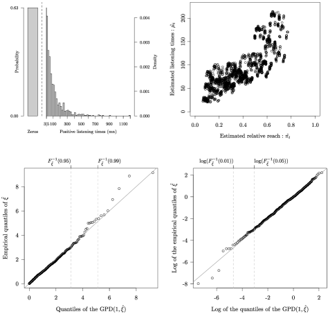
Figure 7: Analyses of listening times to radio “116” in its broadcasting area during the second semester of 2007. Left upper plot: Empirical distribution function. The number of observations is 2155. The clump-at-zero represents the 63% of the data. Right upper plot: Form of the link between the estimated average ratings, $\hat{\pi}_{i}$, and the average listening times, $\hat{\mu}_{i}$. Two bottom plots: QQ-plots of the residuals (left) and of the log of the residuals (right) of the ZITPo model applied to those data. The ordered residuals are compared to the quantiles (left) and to the log of the quantiles (right) of a $\mathrm{GPD}(1,\hat{\xi}=0.082)$.

6 Conclusion

The ZITPo model is a very powerful model that can be used, in particular, to analyze radio audience data. Using the truncated observations, this model allows to adequately estimate the true proportions of nonzero observations and the average of positive values—corresponding to the audience indicators of rating and time spent listening—of the underlying untruncated listening times distribution. The model also allows to relate these expectations to covariates in a GLM spirit, providing an explanatory model to audience data. The model validation procedure resulting from properties of the generalized Pareto distribution offers a very helpful way to judge the adequacy of the model to the data.

Although the main motivation for the development of the ZITPo model was the analysis of radio audience data, we believe that it can adequately fit a number of data sets which have heavy tails distributions. For example, it provides an extension to model (4) for hydrological data, that can include covariates to explain the mean level, with $y^{\circ}=0$.

References

- Aitkin and Clayton (1980) Aitkin, M. and Clayton, D. (1980). The fitting of exponential, Weibull and extreme value distributions to complex censored survival data using GLIM. Appl. Statist. 29 156–163.
- Beirlant, Vynckier and Teugels (1996) Beirlant, J., Vynckier, P. and Teugels, J. L. (1996). Tail index estimation, Pareto quantile plots, and regression diagnostics. J. Amer. Statist. Assoc. 91 1659–1667. \MR1439107
- Castillo and Hadi (1997) Castillo, E. and Hadi, A. S. (1997). Fitting the generalized Pareto distribution to data. J. Amer. Statist. Assoc. 92 1609–1620. \MR1615270
- Chapados et al. (2002) Chapados, N., Bengio, Y., Vincent, V., Ghosn, J., Dugas, C., Takeuchi, I. and Meng, L. (2002). Estimating car insurance premia: A case study in high-dimensional data inference. Advances in Neural Information Processing 14 1369–1376.
- Chavez-Demoulin and Davison (2005) Chavez-Demoulin, V. and Davison, A. C. (2005). Generalized additive modelling of sample extremes. J. Roy. Statist. Soc. Ser. C 54 207–222. \MR2134607
- Chen, Jiang and Mao (2007) Chen, Y., Jiang, Y. and Mao, Y. (2007). Hospital admissions associated with body mass index in Canadian adults. International Journal of Obesity 31 962–967.
- Christmann (2004) Christmann, A. (2004). An approach to model complex high-dimensional insurance data. Allgemeines Statistisches Archiv 88 375–397. \MR2107202
- Coles (2001) Coles, S. (2001). An Introduction to Statistical Modeling of Extreme Values. Springer, London. \MR1932132
- Collett (2003) Collett, D. (2003). Modelling Binary Data. Chapman and Hall, Boca Raton. \MR1999899
- Couturier and Victoria-Feser (2010) Couturier, D.-L. and Victoria-Feser, M.-P. (2010). Supplement to “Zero-inflated truncated generalized Pareto distribution for the analysis of radio audience data.” DOI: 10.1214/10-AOAS358SUPP.
- Davison and Smith (1990) Davison, A. C. and Smith, R. L. (1990). Models for exceedances over high thresholds (with comments). J. Roy. Statist. Soc. Ser. B 52 393–442. \MR1086795
- Duan et al. (1983) Duan, N., Manning, W. G., Morris, C. N. and Newhouse, J. P. (1983). A comparison of alternative models for the demand for medical care. J. Bus. Econom. Statist. 1 115–126.
- Dupuis and Tsao (1998) Dupuis, D. J. and Tsao, M. (1998). A hybrid estimator for generalized Pareto and extreme-value distributions. Commun. Statist. Theory and Methods 27 925–941. \MR1613505
- Dupuis and Victoria-Feser (2006) Dupuis, D. J. and Victoria-Feser, M.-P. (2006). A robust prediction error criterion for Pareto modelling of upper tails. Can. J. Statist. 34 639–658. \MR2347050
- Dähler (2006) Dähler, M. (2006). Vom Fragen zum Messen. Entwicklung und Einführung von Radiocontrol—einem neuen Hörerforschungsinstrument—in der Schweiz. Ph.D. thesis, Faculty of Human Sciences, Univ. Bern. Available at http://www.stub.unibe.ch/download/eldiss/05daehler_m.pdf.
- Hall and Welsh (1985) Hall, P. and Welsh, A. H. (1985). Adaptive estimates of parameters of regular variation. Ann. Statist. 13 330–341. \MR0773171
- Hill (1975) Hill, B. M. (1975). A simple general approach to inference about the tail of a distribution. Ann. Statist. 3 1163–1174. \MR0378204
- Hosking and Wallis (1987) Hosking, J. R. M. and Wallis, J. R. (1987). Parameter and quantile estimation for the generalized Pareto distribution. Technometrics 29 339–349. \MR0906643
- Juárez and Schucany (2004) Juárez, S. F. and Schucany, W. R. (2004). Robust and efficient estimation for the generalized Pareto distribution. Extremes 7 237–251. \MR2143942
- Lambert (1992) Lambert, D. (1992). Zero-inflated Poisson regression, with an application to defects in manufacturing. Technometrics 34 1–14.
- Min and Agresti (2002) Min, Y. and Agresti, A. (2002). Modeling nonnegative data with clumping at zero: A survey. Journal of the Iranian Statistical Society 1 7–33.
- Min and Agresti (2005) Min, Y. and Agresti, A. (2005). Random effect models for repeated measures of zero-inflated count data. Statist. Modell. 5 1–19. \MR2133525
- Mullahy (1986) Mullahy, J. (1986). Specification and testing of some modified count data models. J. Econometrics 33 341–365. \MR0867980
- Nelder and Wedderburn (1972) Nelder, J. A. and Wedderburn, R. W. M. (1972). Generalized linear models. J. Roy. Statist. Soc. Ser. A 135 370–384.
- Peng and Welsh (2001) Peng, L. and Welsh, A. H. (2001). Robust estimation of the generalized Pareto distribution. Extremes 4 53–65. \MR1876179
- Pickands (1975) Pickands, J. (1975). Statistical inference using extreme order statistics. Ann. Statist. 3 119–131. \MR0423667
- Ridout, Demétrio and Hinde (1998) Ridout, M., Demétrio, C. G. and Hinde, J. (1998). Models for count data with many zeros. In International Biometric Conference 179–192. International Biometric Conference, Cope Town.
- Singh and Ahmad (2004) Singh, V. P. and Ahmad, M. (2004). A comparative evaluation of the estimators of the three-parameter generalized Pareto distribution. J. Statist. Comput. Simul. 74 91–106. \MR2037905
- Webster, Phalen and Lichty (2006) Webster, J. G., Phalen, P. F. and Lichty, L. W. (2006). Ratings Analysis. Lawrence Erlbaum Associates, Inc, Publishers, Mahwah, NJ.
- Weglarczyk, Strupczewski and Singh (2005) Weglarczyk, S., Strupczewski, W. G. and Singh, V. P. (2005). Three-parameter discontinuous distributions for hydrological samples with zero values. Hydrological Processes 19 2899–2914.
- Welsh et al. (1996) Welsh, A. H., Cunningham, R. B., Donnelly, C. F. and Lindenmayer, D. B. (1996). Modelling the abundance of rare species: Statistical models for counts with extra zeros. Ecological Modelling 88 297–308.