Single peaked CO emission line profiles from the inner regions of protoplanetary disks

Abstract

Context. Protoplanetary disks generally exhibit strong line emission from the CO fundamental v=1–0 ro-vibrational band around 4.7 $\mu$m. The lines are usually interpreted as being formed in the Keplerian disk, as opposed to other kinematic components of the young stellar system.

Aims. This paper investigates a set of disks that show CO emission line profiles characterized by a single, narrow peak and a broad base extending to $>50\,\rm km\,s^{-1}$, not readily explained by just Keplerian motions of gas in the inner disk.

Methods. High resolution ($R$ = 10⁵) $M$-band spectroscopy has been obtained using CRIRES at the Very Large Telescope in order to fully resolve fundamental ro-vibrational CO emission line profiles around 4.7 $\mu$m.

Results. Line profiles with a narrow peak and broad wings are found for 8 disks among a sample of $\sim$50 disks around T Tauri stars with CO emission. The lines are very symmetric, have high line/continuum ratios and have central velocity shifts of $<$ 5 km s^-1 relative to the stellar radial velocity. The disks in this subsample are accreting onto their central stars at high rates relative to the parent sample. All 8 disks show CO emission lines from the $v=2$ vibrational state and 4/8 disks show emission up to $v=4$. Excitation analyses of the integrated line fluxes reveal a significant difference between typical rotational ($\sim$300-800 K) and vibrational ($\sim$1700 K) temperatures, suggesting that the lines are excited, at least in part, by UV-fluorescence. For at least one source, the narrow and broad components show different excitation temperatures, but generally the two component fits have similar central velocities and temperature. Analysis of their spatial distribution shows that the lines are formed within a few AU of the central star.

Conclusions. It is concluded that these broad centrally peaked line profiles are inconsistent with the double peaked profiles expected from just an inclined disk in Keplerian rotation. Models in which the low velocity emission arises from large disk radii are excluded based on the small spatial distribution. Alternative non-Keplerian line formation mechanisms are discussed, including thermally and magnetically launched winds and funnel flows. The most likely interpretation is that the broad-based centrally peaked line profiles originate from a combination of emission from the inner part ($<$ a few AU) of a circumstellar disk, perhaps with enhanced turbulence, and a slow moving disk wind, launched by either EUV emission or soft X-rays.

1 Introduction

It is generally thought that planets form in the inner regions of protoplanetary disks ($\lesssim$10 AU Lissauer, 1993). Information on the physical structure, gas dynamics and chemical composition of the planet-forming region is essential to constrain models of planet formation. Processes like planet migration, which can change the orbits of newly formed planets, depend sensitively on the presence of gas in the disk (e.g., Ward, 1997; Kley et al., 2009). The planetary mass distributions (Ida & Lin, 2004) and planetary orbits (Kominami & Ida, 2002; Trilling et al., 2002) resulting from planet formation models can eventually be tested against recent observations of exo-planetary systems (e.g., Mordasini et al., 2009a, b). Observations of line emission from disks at high spectral and spatial resolution are needed to provide the initial conditions for these models. Gas-phase tracers of the disk surface can also be used to probe photo-evaporation processes (Gorti et al., 2009; Gorti & Hollenbach, 2009). More generally, these observations provide constraints on the lifetime of the gas in the inner part of the disk and thus its ability to form giant gaseous planets.

The bulk of the gas mass in protoplanetary disks is in H₂ but this molecule is difficult to observe since its rotational quadrupole transitions from low-energy levels are intrinsically weak and lie in wavelength ranges with no or poor atmospheric transmission (e.g., Carmona et al., 2007). In contrast, the next most abundant molecule, CO, has ro-vibrational lines which can be readily detected from the ground. This makes CO an optimal tracer of the characteristics of the warm gas in the inner regions of disks (see Najita et al., 2007, for overview). CO overtone emission ($\Delta{\rm{v}}$ = 2) was detected for the first time in low and high mass young stellar objects by Thompson (1985) and was attributed to circumstellar disks by Carr (1989).

Overtone emission lines at 2.3 $\mu$m from disks around T Tauri stars, when present, have been fitted with double peaked line profiles with a FWHM of around 100 km s^-1, which suggests an origin in the innermost part (0.05-0.3 AU) of the disk under the assumption of Keplerian rotation (Carr et al., 1993; Chandler et al., 1993; Najita et al., 1996). The relative intensities of the ro-vibrational lines can be used to determine characteristic CO excitation temperatures (rotational and vibrational), which, in turn, provide constraints on the kinetic temperatures and densities in the line-forming region. The overtone data resulted in temperature estimates in the 1500-4000 K range and with densities of $>$10¹⁰ cm^-3 (Chandler et al., 1993; Najita et al., 2000, 2007).

Fundamental CO $\rm{v}=1-0$ emission at 4.7 $\mu$m has been observed both from disks around T Tauri stars (e.g., Najita et al., 2003; Rettig et al., 2004; Salyk et al., 2007; Pontoppidan et al., 2008; Salyk et al., 2009) and around Herbig Ae/Be stars (e.g., Brittain et al., 2003; Blake & Boogert, 2004; Brittain et al., 2007, 2009; van der Plas et al., 2009). The fundamental ro-vibrational lines are excited at lower temperatures (1000-1500 K) than the overtone lines (Najita et al., 2007). Fundamental CO emission lines are usually fitted with double peaked or narrow single-peaked line profiles that can be described by a Keplerian model. Single-peaked line profiles with broad wings (up to 100 km s^-1) in T Tauri disks have been seen by Najita et al. (2003), who also discussed their origin. Three possible formation scenarios were mentioned: disk winds, funnel flows or gas in the rotating disk. The latter option was favored, and the lack of a double peak was ascribed to the relatively low ($R$=$\lambda$/$\Delta\lambda$=25000) spectral resolving power of the data. Alternative explanations such as an origin in disk winds and funnel flows were ruled out mainly because of the lack of asymmetry in the line profiles.

The high resolution ($R$ = 10⁵) spectrometer CRIRES (CRyogenic InfraRed Echelle Spectrograph) fed by the MACAO (Multi - Application Curvature Adaptive Optics) adaptive optics system on the Very Large Telescope offers the opportunity to observe molecular gas emission from T-Tauri disks with unsurpassed spectral and spatial resolution. A sample of $\sim$70 disks was observed in the fundamental CO band around 4.7 $\mu$m as part of an extensive survey of molecular emission from young stellar objects. In total, 12 of the 70 T Tauri stars show CO emission lines with a broad base and a narrow central peak, from now on called broad-based single peaked line profiles. Eight of the 12 T Tauri stars are selected for detailed analysis in this paper, based on criteria discussed in §3.5. Because the lines remain single peaked even when observed at 4 times higher spectral resolution than previous observations, the lack of a double peak can no longer be explained by the limited resolution in Najita et al. (2003). Hence the modeled double peaked lines in Najita et al. (2003) are not a plausible explanation for the centrally peaked line profiles in T Tauri disks. The aim of this paper is to classify these broad centrally peaked lines and to constrain their origin. Since many of these sources have high line to continuum ratios and are prime targets to search for molecules other than CO (e.g. Salyk et al., 2008), a better understanding of these sources is also warranted from the perspective of disk chemistry studies.

The observations and sample are presented in $\S$2. In section $\S$3 the line profiles are modeled using a Keplerian disk model where it is concluded that a model with a standard power-law temperature structure does not provide a good fit to the broad-based single peaked line profiles. The profiles are subsequently inverted to determine what temperature distribution would be consistent with the spectra. The origin of the emission is then further constrained in $\S$4 by extracting radial velocity shifts between the gas and the star, determining rotational and vibrational temperatures and investigating the extent of the emission. In $\S$5 the results are discussed and they are summarized in §6.

Table 1: List of sources with single-peaked line profiles analyzed in this paper.

Source	$\alpha$(J2000)	$\delta$(J2000)	Spectral Type	Distance (pc)	Flux [Jy]	$T_{\rm{eff}}$ [K]	$L_{\star}$ [$L_{\odot}$]	Ref.
AS 205 A (N)	16 11 31.4	-18 38 24.5	K5	125	4.0	4250	4.0	1, 4, 8, 10
DR Tau	04 47 06.2	+16 58 42.9	K7	140	1.3	4060	1.1	4, 5, 11
RU Lup	15 56 42.3	-37 49 15.5	K7	140	1.1	4000	1.3	1, 6, 12, 15
S CrA A (N)	19 01 08.6	-36 57 20.0	K3	130	2.2	4800	2.3,	2, 3, 17
S CrA B (S)	19 01 08.6	-36 57 20.0	M0	130	0.8	3800	0.8	2, 3, 17
VV CrA A (S)	19 03 06.7	-37 12 49.7	K7	130	-	4000	0.3	3, 13, 16
VW Cha	11 08 01.8	-77 42 28.8	K5	178	0.7	4350	2.9	7, 9, 14
VZ Cha	11 09 23.8	-76 23 20.8	K6	178	0.4	4200	0.5	7, 9, 14

Table 2: Journal of observations.

Source	Obs. time	Settings ($\mu$m)	Standard star	Spectral type
				standard star
AS 205 A	Apr 07	4.760, 4.662, 4.676, 4.773	BS 4757	A0
	Aug 07	4.730	BS 5812	B2.5
	Apr 08	4.730	BS 6084	B1
	Aug 09	5100, 5115	BS 5984	B0.5
DR Tau	Oct 07	4.716, 4.730, 4.833, 4.868	BS 3117, BS 838	B3, B8
	Dec 08	4.716, 4.946	BS 1791	B7
RU Lup	Apr 07	4.716, 4.730, 4.833, 4.929	BS 5883	B9
	Apr 08	4.730	BS 6084	B1
S CrA	Apr 07	4.730, 4.716	BS 6084	B1
	Aug 07	4.730	BS 7235, BS 7920	A0, A9
	Aug 08	4.868, 4.946	BS 6084, BS 7236	B1, B9
VV CrA A	Apr 07	4.716, 4.730, 4.840	BS 7362	A4
	Aug 07	4.770, 4.779	BS 7236	B9
	Aug 08	4.946	BS 7236	B9
VW Cha	Dec 08	4.716, 4.800, 4.820, 4.946	BS 5571, HR 4467	B2, B9
VZ Cha	Dec 08	4.716, 4.800, 4.820, 4.946	BS 5571, HR 4467	B2, B9

2 Observations and sample

A sample of 70 disks around low-mass pre-main sequence stars was observed at high spectral resolving power ($\lambda/\Delta\lambda$ = 10⁵ or 3 km s^-1) with CRIRES mounted on UT1 at the Very Large Telescope (VLT) of the European Southern Observatory, Paranal, Chile. The CRIRES instrument (Käufl et al., 2004) is fed by an adaptive optics system (MACAO, Paufique et al., 2004), resulting in a typical spatial resolution of $\sim$160-200 milli-arcsec along the slit. CRIRES has 4 detectors that each cover about 0.02 – 0.03 $\mu$m with gaps of about 0.006 $\mu$m at 4.7 $\mu$m. Staggered pairs of settings shifted in wavelength are observed to cover the detector gaps and produce continuous spectra.

The observations were taken during a period from April 21 2007 to January 3 2009. The parent sample is a broad selection of low-mass young stellar objects, consisting mostly of T Tauri stars and a few Herbig Ae stars. The full data set will be published in a future study (Brown et al. in prep.). Of the 70 sources, about 50 disks around T Tauri stars show clear CO emission lines. This paper focuses on a subsample of 8 of the 12 objects that show broad-based single peaked CO ro-vibrational line profiles. Their names and characteristic parameters are presented in Table 1, and their selection is justified in §3.2 and §4. Inclinations are unknown for the majority of the sources. Several of the sources in the sample are binaries, with the primary and secondary defined as A and B, respectively. The specific definition for each source’s primary and secondary is taken from the literature, see Table 1. For S CrA, both A and B components show broad-based centrally peaked line profiles. For AS 205 and VV CrA, only the A component has such single-peaked emission profiles. The B components show CO absorption (see Smith et al. 2009 for the case of VV CrA B). Thus, there is no obvious trend of the presence of these profiles with binarity of the system.

Ground-based M-band spectroscopy is usually dominated by strong sky emission lines (including CO itself) superimposed on a thermal continuum. Nodding with a throw of 10” was performed to correct for both the sky emission and the thermal continuum. In addition jittering with a random offset within a radius of 0$\aas@@fstack{\prime\prime}$5 was used to decrease systematics and to remove bad pixels. The weather conditions during the observations were usually good with optical seeing varying typically between 0$\aas@@fstack{\prime\prime}$5 – 1$\aas@@fstack{\prime\prime}$5. Even at times when the seeing was higher most of the light still passed through the 0$\aas@@fstack{\prime\prime}$2 slit because of the adaptive optics system. Observations of standard stars were done close in time to each science target with airmass differences of typically 0.05–0.1 in order to correct for telluric features.

The observations typically covered CO $\rm{v}=1-0$: R(8)–P(32) lines, where the notation indicates that most lines between R(8) and P(32) are observed, including, for example, the R(0) and P(1) lines. Lines from vibrationally excited levels as well as isotopologues are also included, specifically: CO $\rm{v}=2-1$: R(17)–P(26); CO $\rm{v}=3-2$: R(26)–P (21); CO $\rm{v}=4-3$: R(37)–P(15); ¹³CO: R(24)–P(23); C¹⁸O: R (17)–P(27); and C¹⁷O: R(26)–P(22).

The wavelengths and dates of the observations can be found in Table 2. Each wavelength setting is centered on the third, in order of increasing wavelength, of the four detectors. As an example, the setting at 4.730 $\mu$m corresponds to a spectral range of 4.660 – 4.769 $\mu$m. Observations were sometimes taken during different seasons to shift the telluric lines relative to the source spectrum due to the reflex motion of the Earth. Combination of the two data sets then allows the reconstruction of the complete line profile, whereas a single epoch would have a gap due to the presence of a saturated telluric CO line. For 6 of the sources presented here, no evidence has been found that the line fluxes and profiles changed within this 1–1.5 yr period. For VW Cha and VZ Cha this information is not available since they were only observed once.

2.1 Data reduction

Figure 1: Part of the VLT-CRIRES spectrum of AS 205 A. The strong ¹²CO lines are labelled with their $R$-band lower $J$-transition number and the other marked lines show detections of ¹²CO $\rm{v}$ = 2–1, $\rm{v}$ = 3-2, ¹³CO, and the Pfund-$\beta$ line. The gaps in the spectrum are excised telluric features. For other parts of the AS 205 A spectrum, these gaps have been filled in by observations at different times of the year (see Fig. 2).

The spectra were reduced using standard methods for infrared spectroscopy (see Pontoppidan et al., 2008, for details). Dome flats were used for each setting to correct the images for pixel-to-pixel sensitivity differences in the detectors. A linearity correction was applied to the frames using the parametrization given in the CRIRES documentation. The nod pairs were then differenced to subtract the background. The data stack was co-added after correction for field distortion. Extraction of the 2-dimensional images to 1 dimensional spectra was done after the subtraction and combination of the 2-D frames tracing the source in the 2-D spectra. Additional spectra of well separated binaries were extracted as well during this procedure.

The spectra were subsequently wavelength calibrated by fitting the standard star atmospheric lines to an atmospheric model generated using the Reference Forward Model (RFM) code. This model is a line-by-line radiative transfer model developed at Oxford University based on Clough et al. (1982). The typical velocity accuracy is about 0.1–1 km s^-1, but can vary between settings, depending on the density of telluric lines. The last step in the reduction process was to correct for the strong telluric absorption lines in the spectra, by dividing the science spectra with the spectra taken of early-type photospheric standard stars. These hot stars have a strong hydrogen Pfund $\beta$ (7-5) absorption line at 4.654 $\mu$m. Division by the standard star therefore introduces an artificial contribution to the emission line in the science spectra. However, Pfund $\beta$ is detected in emission towards most of the sources prior to telluric correction. Early-type photospheric standard stars are otherwise rather featureless throughout the spectral band. Flux calibration was carried out by scaling to photometry from the Spitzer IRAC band 2 (see Table 1).

Figure 2: Partial spectra for the entire sample of sources with single peaked ¹²CO lines. The HI Pfund $\beta$ line at 4.655 $\mu$m is included. The spikes seen in spectra of S CrA A, B and VV CrA A are narrow (self) absorption lines visible in the low $J$ lines.

In Fig. 1 part of the reduced spectrum for the northern of the binary components of AS 205 is presented. This spectrum shows highly resolved ¹²CO line profiles for the ${\rm v}=1-0$ transitions R(8)–R(0) and clear detections of ¹³CO v$=1-0$, CO $\rm{v}=2-1$ and $\rm{v}=3-2$ lines and the Pfund $\beta$ line. An overview of parts of the spectra of the 8 single peaked sources is presented in Fig. 2.

3 Line profiles

3.1 ¹²CO line profiles

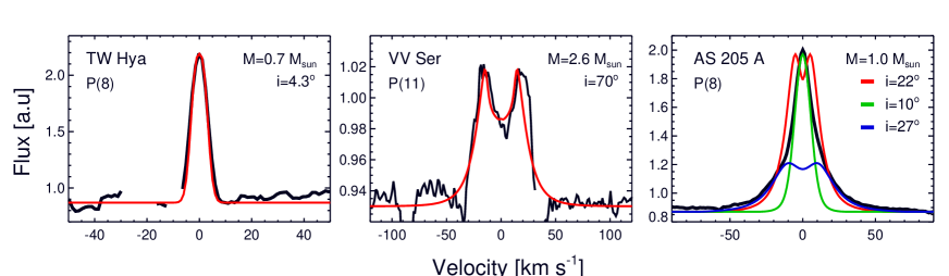
Figure 3: Modeled lines, plotted in red, are fitted to observed spectral lines in black of TW Hya, VV Ser and AS 205 A. Good fits could be found for VV Ser and TW Hya using a Keplerian model with a power-law temperature profile. No good fits could be found for AS 205 A. The optimal fit to the total line profile (red) using extended emission out to 10 AU, to the narrow inner part (green) and to the outer broader wings (blue) are presented in the right figure. See text for model parameters.

The spectrally resolved fundamental CO emission lines from the sample of T Tauri stars observed with CRIRES show a broad variety of profiles. Often, the line profiles can be explained by Keplerian rotation, absorption by the disk or absorption by a foreground cloud (Brown et al., in prep). Fig. 3 shows a selection of emission line profiles of three basic shapes: A) narrow single-peaked, matched by a single Gaussian, B) double-peaked line profiles and C) single-peaked with broad wings. Lines that show absorption are not included due to the difficulty in determining the profile close to line center.

The CO line profiles of TW Hya fall in category A and likely arise from gas in a face-on disk in Keplerian rotation (e.g. Pontoppidan et al., 2008). Prototypical for category C are the line profiles of the source AS 205 A, which are by inspection qualitatively different from the double peaked profiles of sources like AA Tau and VV Ser (category B) because of their single narrow peak relative to a broad base. While categories A and B appear to be well understood (see below), the question is what the origin of the broad centrally peaked line profiles of category C is.

3.2 Keplerian disk model

To investigate to what extent the broad centrally peaked (category C) line profiles can be described by emission originating from gas circulating in the inner parts of the disk, a simple disk model of gas in Keplerian rotation adopted from Pontoppidan et al. (2008) is used.

3.2.1 Description of the model

The model includes a flat disk with constant radial surface density. The motions of the gas in the disk are described by Kepler’s law. The disk is divided into emitting rings with radial sizes that are increasing logarithmically with radius. Each ring has a specific temperature. Local thermal equilibrium (LTE) is used as an approximation for describing the excitation of the emitting molecules, which means that the relative populations in a ro-vibrational level can be derived using the Boltzmann distribution at the given temperature in each emitting ring.

In the standard formulation, a power law is used to describe the temperature gradient throughout the disk, $T=T_{0}(R/R_{0})^{-\alpha}$, where $T$ is the gas temperature, $R$ is the radius and $T_{0}$ is the temperature at the inner radius $R_{0}$. The other parameters are: the mass of the star $M_{\star}$; the inclination of the disk $i$; the outer radius of the disk $R_{\rm{max}}$; and a line broadening parameter $\Delta{V}_{\rm{mod}}$ which combines the instrumental broadening and any turbulent broadening. Several parameters are degenerate, including the stellar mass and disk inclination. Thus, this model is not used to derive the best estimates of the characteristic parameters of the sources. The aim is instead to explore the parameter space to see whether good fits can be found for the category C line profiles using basic Keplerian physics. The local line profile is convolved with a Gaussian turbulent line FWHM broadening ($\Delta{V}_{\rm{turb}}$) which describes the local turbulence of the gas in the disk. The instrumental broadening ($\Delta{V}_{\rm{instr}}$) can also be represented by a Gaussian, which has a FWHM value of 3 km s^-1 for CRIRES. The lowest value for $\Delta{V}_{\rm{mod}}=(\Delta{V}_{\rm{turb}}^{2}+\Delta{V}_{\rm{instr}}^{2})^{1/2}$ is therefore set to 3 km s^-1 and any additional broadening represents an increase in the value of $\Delta{V}_{\rm{turb}}$. For temperatures up to 1000 K, typical of the molecular gas in the inner disk, the thermal broadening of the CO lines of up to 1.3 km s^-1 is negligible.

3.2.2 Fits with a Keplerian model with a power-law temperature profile

The sources TW Hya, VV Ser and AS 205 A were chosen as illustration since their fundamental CO emission lines represent the three main different types of line profiles in our large sample. Each of these sources and their fits are presented here and shown in Fig. 3.

Single peaked narrow line profile – TW Hya: A good fit was found to the narrow single peaked line profile of the TW Hya disk. This fit was achieved by using a low inclination angle of $i$ = 4.3$\degr$, $\alpha$ = 0.4, a stellar mass of 0.7 M_⊙, $R_{0}$ = 0.1 AU, $T_{0}$ = 1100 K, $R_{\rm{max}}$ = 1.5 AU and $\Delta{V}_{\rm{mod}}=$3 km s^-1, see the left plot in Fig. 3. The adopted stellar mass and disk inclination are taken from Pontoppidan et al. (2008). For this source, CO emission from the Keplerian disk model described above, convolved to the 3 km s^-1 instrumental resolution of CRIRES, provides a good fit to all lines. Additional line broadening from turbulence is not needed to explain the line profiles. This low turbulence is consistent with the low turbulent velocity of $\sim$0.1 km s^-1 inferred for the outer disk of TW Hya by Qi et al. (2006), although that value refers to much cooler gas at large radii in the disk.

Double peaked line profile – VV Ser: VV Ser is an example of a disk with double peaked line profiles extending out to velocities of $\pm$ 40 km s^-1. VV Ser is a Herbig Ae/Be star of spectral type A2-B6 with a mass of 2.6 $\pm$ 0.2 M_⊙ and an inclination of 65-75^o (Pontoppidan et al., 2007). A good fit between the model and the data is shown in the center panel in Fig 3. The estimated parameters are $M_{\star}$ = 2.6 M_⊙, $i$ = 70$\degr$, $T_{0}$ = 3500 K, $\alpha$ = 0.45, $R_{0}$ = 0.08 AU, $R_{\rm{max}}$ = 11 AU and $\Delta{V}_{\rm{mod}}=$3 km s^-1. However in this case the parameter space is rather large since smaller inclination angles will give equally good fits if a higher stellar mass is used. The main point here is that a good fit can readily be obtained with reasonable parameters for a Keplerian model.

Single peaked broad-based line profile – AS 205 A: No equally good fit could be found for the emission lines from AS 205 A. An approximate fit is shown in red in the right plot of Fig. 3 with a model using an inclination angle of $i$ = 22$\degr$, $R_{0}$ = 0.04 AU, $R_{\rm{max}}$ = 5 AU, $\Delta{V}_{\rm{mod}}=$3 km s^-1, $T_{0}$ = 1100 K, $\alpha$ = 0.3, and a mass of 1.0 M_⊙. The mass is the same and the inclination angle is close to that given by Andrews et al. (2009, 1.0 M_⊙ and 25$\degr$, respectively). As for TW Hya, the millimeter data of Andrews et al. (2009) refer to much larger radii (typically $>$50 AU) than the CRIRES observations that the model is fitted to. A lower inclination angle of 10$\degr$ gives a better fit to the narrow central part of the line but results in poor fitting of the outer wings of the profile, as presented by the green profile in Fig. 3. The blue line represents the best fit to the line wings, which is achieved by increasing the inclination angle to 27$\degr$ and taking $\alpha$ to be 0.36.

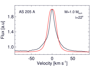
Figure 4: Fit to the broad-based single peaked line of AS 205 A (black) using a standard Keplerian model with a power-law temperature profile (red) including an enhanced line broadening parameter ($\Delta{V}_{\rm{mod}}$) of 8 km s^-1. The other parameters are $i$ = 22$\degr$, $R_{0}$ = 0.04 AU, $R_{\rm{max}}$ = 5 AU, $T_{0}$ = 1100 K, $\alpha$ = 0.3 and a mass of 1.0 M_⊙ (as in $\S$3.2.2).

One option to improve the fit to the AS 205 A data could be to increase the turbulent broadening so that the central dip is filled in. Indeed, increasing $\Delta V_{\rm mod}$ to 8 km s^-1, removes the central double peak (see Fig. 4). This fit is unable to simultaneously match both the narrow peak and the broad base of the profile, however.

In summary, the fits to TW Hya and VV Ser show that both narrow single peaked and double peaked line profiles can be reproduced with a simple Keplerian model with reasonable parameters. However a single peaked line with broad wings cannot be well explained with this type of standard Keplerian model as long as the temperature gradient is described by a continuous power-law.

3.2.3 Keplerian disk models with a non-standard temperature profile

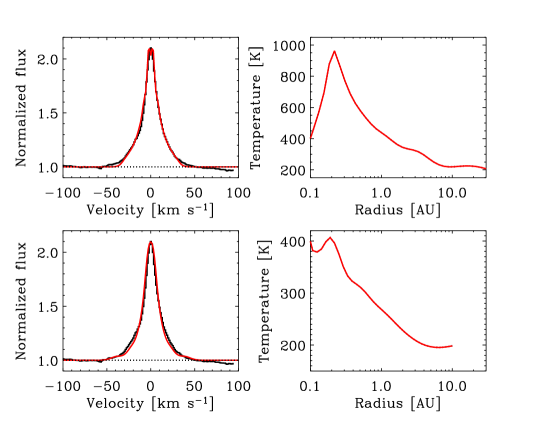
Figure 5: Left panel: Keplerian model (red) using an iterative inversion method to fit the velocity profile of the AS 205 A CO $\rm{v}=1-0$ P(8) line (black). Right panel: The excitation temperature as a function of radius needed to create the modeled lines. The models in the upper panels include extended emission out to 30 AU, a stellar mass of 1.4 M_⊙, an inclination of 25$\degr$ and $\Delta V_{\rm mod}$=3 km s^-1. The models in the lower panels include emission out to 10 AU, a stellar mass of 1.0 M_⊙, an inclination of 22$\degr$ and an increased $\Delta V_{\rm mod}$=7 km s^-1.

Since disk models with a standard temperature and density power-law do not fit the data, one complementary approach is to investigate what physical distribution would be needed to reproduce the line profiles within a Keplerian model. For this, an iterative approach is used in which the observed line profile is ‘inverted’ to determine the temperature distribution that would be consistent with the data. Specifically, the disk is divided into rings and the temperature of each ring is adjusted to match the line profile. The left panels of Fig. 5 present the model compared with the velocity profile of the AS 205 CO ${\rm v}=1-0$ P(8) line whereas the right plots show the corresponding excitation temperature profiles with radius. For LTE excitation and optically thin emission, the latter can also be viewed as an intensity profile with radius. The upper plots use the same parameters as in $\S$3.2.2 for AS 205 A but with a higher stellar mass of 1.4 M_⊙, a higher inclination angle of $i$=25°and including extended emission out to 30 AU. The lower plots show a model using the same parameters as in $\S$3.2.2 but with an extended emission out to 10 AU and increasing the $\Delta V_{\rm mod}$ to 7 km s^-1. Both of these models fit the line profiles well, illustrating that a Keplerian disk model with an unusual temperature distribution can explain the data. The emission is much more extended, however, than in the case of the standard disk models with a power-law temperature profile: out to 30 AU in the case of no turbulence or out to 10 AU with increasing $\Delta V_{\rm mod}$. These models will be further tested in $\S$5.1 using the constraints on the spatial extent of the observed emission found in $\S$4.3.

Figure 6: The line profile parameter $P_{10}$=$\Delta{V}_{10}$/$\Delta{V}_{90}$ is presented here for a sample of selected sources. Note that this parameter is clearly larger for the broad-based single peaked line profiles. The $P_{10}$-value is an average of the lower $J$-transition lines (up to P(14)). The $J$-transition corresponding to each plotted profile is given in the figure. The narrow absorption line seen toward DoAr24E A is due to ¹³CO absorption in the foreground cloud.

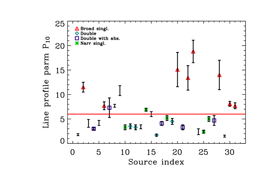
Figure 7: The line profile parameter $P_{10}$ for different sources. The index numbers represent the different sources, see Table 1. Each type of line profile is given by a specific symbol. Data points without a symbol are for sources without clearly defined line profiles. The red line gives the maximum line profile parameter achieved using a standard Keplerian disk model with a power-law temperature profile.

Table 3: The peakiness parameter $P_{10}$, the accretion luminosity and the line/continuum ($L/C$) ratio for a selected sample of protoplanetary disks.

Index number	Source	$P_{10}$	$L/C$	Acc. lum.	Ref.
				[log(L⊙)]
1	AA Tau	1.8 (0.2)	1.5	-1.6	1
2	AS 205 A	11.5 (1.0)	2.1	0.2	2
3	CV Cha	4.1 (0.8)	1.3	-	-
4	CW Tau	3.0 (0.2)	1.4	-1.3	2
5	DF Tau	4.2 (0.5)	1.5	- 0.7	3
6	DR Tau	7.7 (0.8)	2.9	- 0.1	2
7	DoAr24E A	7.3 (2.0)	1.5	- 1.6	4
8	DoAr 44	7.7 (0.3)	1.4	-	-
9	EX Lup	10.8 (1.0)	1.3	-	-
10	FN Tau	3.3 (0.5)	1.5	-	-
11	GQ Lup	3.5 (0.5)	1.4	-	-
12	Haro 1-4	3.3 (0.5)	1.4	-	-
13	Haro 1-16	3.4 (0.4)	1.3	-	-
14	HD135344B	6.9 (0.3)	1.2	-0.9	5
15	HD142527	6.0 (0.5)	1.2	0.0	5
16	IRS 48	1.7 (0.2)	1.2	-	-
17	IRS 51	4.1 (0.4)	1.2	-	-
18	LkHa 330	5.2 (0.5)	1.3	-	-
19	RNO 90	4.5 (0.6)	1.5	-	-
20	RU Lup	15.1 (3.5)	1.8	- 0.4	3
21	RY Lup	3.3 (0.5)	1.2	-	-
22	S CrA A	13.4 (2.5)	2.0	-	-
23	S CrA B	18.8 (2.3)	1.8	-	-
24	SR 9	2.4 (0.6)	1.1	-1.4	4
25	SR 21	2.4 (0.3)	1.2	$<$-1.9	4
26	TW Hya	5.0 (0.5)	2.3	-1.4	3
27	VSSG1	4.7 (1.0)	1.5	- 0.4	4
28	VV CrA A	14.0 (3.0)	1.4	-	-
29	VV Ser	1.5 (0.2)	1.1	1.2	5
30	VW Cha	8.1 (0.5)	2.0	- 0.2	6
31	VZ Cha	7.7 (0.6)	2.2	- 1.1	6

3.3 Line profile parameter

A parameter is defined to quantify the difference in line profiles between the broad single peaked sources (category C) and the other sources in the sample. This so-called line profile parameter $P_{10}$ describes the degree to which line profiles have a broad base relative to their peak. The line profile parameter $P_{10}$ is therefore defined as the full width ($\Delta{V}_{10}$) of the line at 10% of its height divided by the full width at 90% ($\Delta{V}_{90}$) of its height, $P_{10}$ = $\Delta{V}_{10}/\Delta{V}_{90}$. The broad-based single peaked lines (category C) have a higher value of the line profile parameter relative to the double and narrow single peaked lines, see Fig. 6.

A summary of the line profile parameter values for 31 selected T Tauri stars from the total sample of $\sim$50 T Tauri stars with CO emission is presented in Fig. 7 and Table 3. These 31 T Tauri stars were selected because their CO emission line profiles have high $S/N$ and are not contaminated by strong telluric or absorption lines. Figure 7 shows that the double peaked (turquoise diamonds) and narrow single peaked (green stars) sources all have a line profile parameter of $<$6. For reference, a Gaussian line profile has a $P_{10}$-value of 4.7. The selected sample of 8 broad centrally peaked sources (red triangles) all have a $P_{10}$-value of $>$6. An overview of the normalized and continuum-subtracted ¹²CO P(8) line profiles of this subset is presented in Fig. 8. These lines are typically symmetric around line center and have a narrow top and a very broad base that extends out to $\pm$100 km s^-1 in several cases. Four other sources, DoAr24E A, DoAr44, EX Lup and HD135344B, also have higher ($>$6) $P_{10}$- values but are not selected for our sample (see $\S$3.5 for source selection criteria).

Figure 8: The P(8) ¹²CO line is plotted for the entire sample broad-based single peaked sources, apart from VW Cha for which the P(10) line is presented because the P(8) line is affected by a strong telluric feature at the time of observation. The lines have been continuum subtracted and normalized. The asymmetry of the VV CrA A line is caused by line blending by the CO $\rm{v}=3-2$ R(5) line. This line overlap adds intensity on the blue side of the ¹²CO P(8) line.

3.4 Model line profile parameters

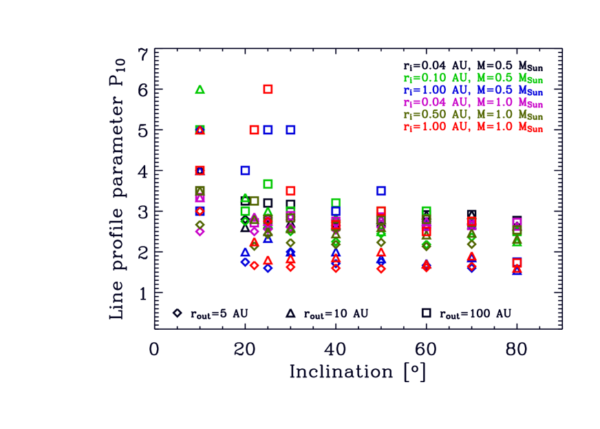
Figure 9: Line profile parameter $P_{10}$ versus inclination for a large model grid of standard Keplerian models with a power-law temperature profile. Note that $P_{10}$ does not become larger than 6 and shows no trend with inclination for $i>20^{o}$.

To derive the maximum line profile parameter consistent with a standard Keplerian model with a power-law temperature profile, a grid of Keplerian line profiles was constructed. Three parameters in the model were set to fixed values that give strongly peaked line profiles; $T_{0}$ = 1100 K, $\alpha$ = 0.30 and $\Delta{V}_{\rm{mod}}$ = 3 km s^-1. The following parameters were varied between $M_{\star}$ = 0.5 – 1.0 M_⊙, $i$ = 10 – 80$\degr$, $R_{0}$ = 0.04 – 1.0 AU and $R_{\rm{max}}$ = 5 – 100 AU and the $P_{10}$- value was calculated for each produced line profile. An overview of the $P_{10}$-values versus inclination is shown in Fig. 9. It is found that a typical standard Keplerian model with a power-law temperature profile can achieve a maximum $P_{10}$-value of about 6, with the highest values found at low inclination. This conclusion is unchanged if $\Delta V_{\rm mod}$ is increased to values as large as $\sim$10 km s^-1. The upper limit of $P_{10}\approx$ 6 that the Keplerian model can reproduce is presented as a red line in Fig. 7. Figure 9 also indicates that the inclination of the source, invoked to explain the different widths of Herbig Ae disk profiles (Blake & Boogert, 2004), should not affect the value of $P_{10}$ significantly except at very low inclinations, since it enters both $\Delta{V}_{10}$ and $\Delta{V}_{90}$.

Note that the Keplerian models always require a low inclination angle of 20 – 30$\degr$ to obtain high values of the line profile parameter $P_{10}$, regardless of whether or not a large turbulent broadening is included. If inclination angles within 5$\degr$ of the range $i$ = 20 – 30$\degr$ are considered necessary for the broad single peaked line profiles, then 6 $\pm$ 3 sources of the total sample of 50 T Tauri stars would have broad, single-peaked line profiles, which is consistent with our subsample of 8 sources. Millimeter interferometry data for AS 205 A and DR Tau yield inclinations of 25$\degr$ and 37$\pm$ 3$\degr$, respectively (Andrews, 2008; Andrews et al., 2009; Isella et al., 2009), which are roughly consistent with the model requirements.

3.5 $P_{10}$-value versus the line-to-continuum ratio and source selection.

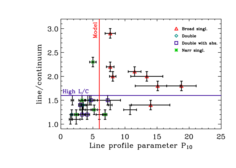
Figure 10: The line to continuum ratio relative to the line profile parameter $P_{10}$. Each type of line profile is given by a specific symbol. Data points without a symbol do not have a clearly defined line profile. The broad single peaked sample includes sources with either a line/continuum ratio $>$ 1.6 (blue line) and $P_{10}>6$ (red line) or solely $P_{10}>10$.

The broad-based single peaked sources are also noteworthy for having high line-to-continuum ($L/C$) ratios in many lines, including the resolved CO ro-vibrational lines discussed here and H₂O lines in Salyk et al. (2008). Here, the $L/C$-ratio is defined as the ratio between the peak line flux relative to the continuum flux. The $L/C$ ratios of the ¹²CO lines have been plotted against the $P_{10}$-values in Fig. 10. Typical uncertainties of the line-to-continuum ratio are $\pm$0.1. Seven of the sources stand out clearly with high line profile parameters and high line-to-continuum ratios. Figure 10 is used to set the criteria ($P_{10}$ $>$ 6 and $L/C$ $>$ 1.6) for the selection of the broad-based single peaked line profiles (category C). The lower limit for the $P_{10}$-value ($P_{10}$ $>$ 6) for the sample is set to match the maximum line profile parameter for a line that the standard Keplerian model with a power-law temperature profile can produce (§3.4). The line-to-continuum constraint of $L/C$ $>$ 1.6 is rather arbitrary, based on the observation that the majority of the sources have a lower value. Two other sources, EX Lup and VV CrA A, have $L/C$ ratios less than 1.6 but have such a high line profile parameter ($>$10) that they are considered to belong to the category C profile sample. However, EX Lup is a variable source that underwent an outburst in 2008. The variation of the CO line profiles from EX Lup during and after the outburst are discussed in Goto et al. (subm.). DoAr 44 and DoAr24E A are borderline cases and are not included here because their profiles are contaminated by absorption, limiting the analysis. HD135344B is also excluded from the sample due to the combination of having both a low $L/C$ ratio and a $P_{10}$-value close to 6. In addition HD135344B is a well-known face-on disk whose profile has been well fitted with a Keplerian model (Pontoppidan et al., 2008; Brown et al., 2009; Grady et al., 2009). Line profiles emitted by disks with a low inclination angle can have a line profile parameter close to 6, as shown in Fig. 9. These selection criteria yield in total 8 sources that are included in the broad-based single peaked sample; these sources are marked with red triangles in Fig. 10.

4 Characteristics for the sources with broad single peaked lines

In §3, we showed that our selected sources with broad single peaked line profiles (category C) cannot be reproduced well with a standard Keplerian model with a power-law temperature profile. In the following sections, we analyze the observational characteristics of the emission to obtain further constraints on the origin.

4.1 Line profiles of CO isotopologues and the $\rm{v}=2-1$ CO lines.

Table 4: List of CO isotopologues and the ¹²CO $\rm{v}=2-1$, $\rm{v}=3-2$ and $\rm{v}=4-3$ lines.

Source	12CO	13CO	CO $\rm{v}=2-1$	CO $\rm{v}=3-2$	CO $\rm{v}=4-3$	C18O
AS 205 A	x	x	x	x	x	x
DR Tau	x	x	x	x	x	x
RU Lup	x	x	x	x	-	-
S CrA A	x, a	x	x	x	x	x
S CrA B	x, a	x	x	x	-	-
VV CrA A	x, a	x, a	x	x	x	a
VW Cha	x	a	x	-	-	-
VZ Cha	x	-	x	x	-	-

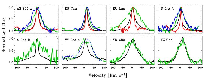
Figure 11: ¹³CO (red), CO $\rm{v}=2-1$ (green) and $\rm{v}=3-2$ (blue) line are plotted on top of the CO $\rm{v}=1-0$ lines (black) for the broad-based single peaked CO emitting sample of T Tauri stars. Dashed lines indicate that the line profile is constructed by stacked lines that all are to some degree affected by line overlap. All profles have been normalized to a peak flux of unity.

Table 4 summarizes the lines seen in the spectra of the broad single peaked sources, including if they are detected in absorption, emission or both. In the richest spectrum, that of AS 205 A, lines of ¹³CO, C¹⁸O, CO $\rm{v}=1-0$, $\rm{v}=2-1$, $\rm{v}=3-2$ and $\rm{v}=4-3$ are all detected. All of the sources, besides VZ Cha, have detections of ¹³CO. Four sources have a C¹⁸O detection in emission. In addition every source in the sample has detections of CO $\rm{v}=2-1$, 7 of 8 sources of CO $\rm{v}=3-2$ and 4 of 8 sources of CO $\rm{v}=4-3$.

Fig. 11 compares the stacked, normalized and continuum-subtracted line profiles for ¹³CO $\rm v=1-0$, ¹²CO $\rm v=1-0$, ¹²CO $\rm v=2-1$ and ¹²CO $\rm v=3-2$. All of the isotopologues and the higher ro-vibrational transitions also show a broad-based single peaked line profile. However, the profiles of the ¹²CO and ¹³CO $\rm v=1-0$ lines match exactly for only one source, AS 205 A. For the other sources, DR Tau, RU Lup, and S CrA A, the ¹³CO lines are narrower than the ¹²CO $\rm v=1-0$ lines.

The width of the CO $\rm{v}=1-0$ lines at 10% of their height (see Table 6) are in general narrower than the CO $\rm{v}=2-1$ and $\rm{v}=3-2$ lines by about 60-80% which can be seen in Fig. 11. Najita et al. (2003) also found a similar trend of broader higher vibrational lines in their data. The difference in width between the lower and higher vibrational lines in our sample may reflect a physical difference in the location of the emitting gas. The high fraction of CO $\rm{v}=2-1$ and $3-2$ detections in our sample of broad-based single peaked line sources is consistent with the Najita et al. (2003) sample, where 9 of their 12 CO sources have detections of $\rm{v}=2-1$ emission and 3 out of 12 sources have $\rm{v}=3-2$ detections. However it is difficult to categorize their line profiles due to the lower spectral resolution.

4.1.1 Two component fits

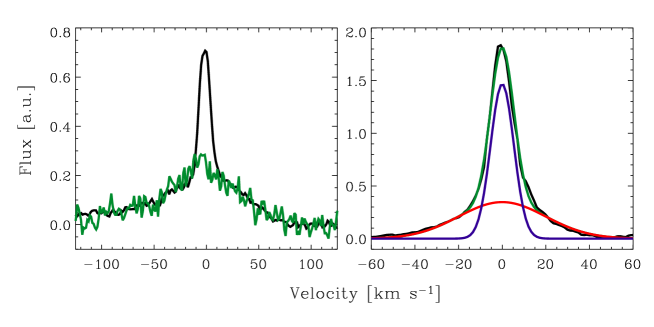
Figure 12: Left: The higher $J$-transition ¹²CO P(32) (green) is plotted on top of the lower $J$-transition ¹²CO P(8) (black) for S CrA B. The narrow component of the ¹²CO P(8) line decreases with increasing excitation. Right: Two Gaussian fitted lines (in red and blue) to the CO $\rm{v}=1-0$ P(7) line of DR Tau (black). The green line represents the sum of the two Gaussian fits.

Table 5: The FWHM of the broad and narrow components and their average heliocentric velocities $V_{B}$(CO) and $V_{N}$(CO) relative to literature values of the heliocentric velocities for the stars $V_{h}$(star).

Source	FWHMB	FWHMN	$V_{B}$(CO)	$V_{N}$(CO)	$V_{h}$(star)	Ref.
	km s-1	km s-1	km s-1	km s-1	km s-1
AS 205 A	61.3 (16.3)	14.8 (1.7)	-4.4 (4.8)	-6.2 (0.3)	-9.4 (1.5)	1
DR Tau	39.8 (6.3)	13.1 (0.9)	26.9 (1.3)	24.4 (0.7)	27.6 (2.0)	3
RU Lup	96.8 (11.0)	24.0 (3.9)	0.4 (7.0)	-3.9 (1.1)	-0.9 (1.2)	1
S CrA A	50.2 (6.7)	10.7 (1.2)	-9.2 (1.4)	-5.0 (0.7)	0.9 (0.9)	2
S CrA B	97.6 (17.7)	12.3 (0.5)	-4.7 (3.5)	-3.5 (0.3)	0.9 (0.9)	2
VV CrA A	-	19.3 (2.0)	-	-0.9 (0.2)	-	-
VW Cha	70.6 (3.1)	26.6 (2.2)	15.4 (1.4)	15.1 (1.9)	17. 2 (2.0)	2
VZ Cha	45.1 (2.6)	-	19.1 (1.7)	-	16.3 (0.6)	2

The line profiles shown in Fig. 8 are generally not well fit by a single Gaussian profile. A good example of this is the CO emission line profiles of S CrA B, which clearly consist of two components. An interesting aspect is that the narrow component stands out very prominently in the low $J$-transitions but progressively decreases in intensity with higher $J$-transitions relative to the broad component (Fig. 12). The simplest explanation is that the components arise from different locations where the narrow component has a lower rotational temperature than the broad component. This is not as clearly seen for the other 7 sources in the sample. However, Najita et al. (2003) see a similar phenomenon in the broad-based single peaked source GW Ori.

The line profiles from S CrA A and GW Ori support a hypothesis in which two physical components combine to form broad centrally peaked line profiles. We therefore fit the line profiles of all sources with two Gaussians to investigate the possibility that the broad-based centrally peaked line profiles consist of two physical components. In the fits, all 6 Gaussian parameters (the two widths, amplitudes and central wavelengths) are left free. For example, Fig. 12 shows that the CO $\rm{v}=1-0$ P(7) line from DR Tau is well-fit with two Gaussian profiles, one narrow and one broad.

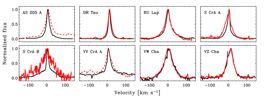
Figure 13: Comparison of the lower $J$ and higher $J$ profiles. The red line represents the stacked higher $J$-transitions ($J$ = P(22)-P(32)) and the black line the lower $J$-transitions (up to $J$ = P(14)) of $\rm{v}=1-0$ CO. The baseline for the higher stacked $J$-transitions for AS 205 A and VV CrA A (dashed red) is not straight because of line overlap and blend. All profiles have been normalized to a peak flux of unity.

Table 6: The averaged line profile parameter $P_{10}$ for high and low $J$-transitions for the sample of sources with single peaked CO $\rm{v}=1-0$ emission lines. $\Delta{V_{10}}$ is the averaged width of the line at 10% of its height.

	$P_{10}$
Source	(low $J$)	(high $J$)	$\Delta{V_{10}}$ [km s-1]
AS 205 A	11.5 (0.5)	-	62.8 (3.9)
DR Tau	7.7 (0.8)	6.6 (0.6)	40.2 (1.0)
RU Lup	15.1 (3.5)	10.5 (2.3)	109 (11.1)
S CrA A	13.4 (2.5)	7.9 (0.2)	56.9 (3.4)
S CrA B	18.8 (2.3)	12.5 (1.0)	102.6 (6.9)
VW Cha	8.1 (0.5)	8.4 (0.3)	115.0 (7.0)
VZ Cha	7.7 (0.6)	7.7 (0.9)	79.2 (2.4)

Two Gaussian profiles are needed for 7 of the 8 broad-based single peaked sources to find an optimal fit to their line profiles. The resulting FWHM_B, FWHM_N, $V_{B}$(CO) and $V_{N}$(CO) are presented in Table 5. These results show that the broad-based single peaked line profiles (category C) can be fitted using a narrow component with a FWHM varying between $\sim$ 10 - 26 km s^-1 and a broad component with FWHM of $\sim$ 40 - 100 km s^-1. The central velocities of the two components are generally the same within the errors. Only the line profile of VZ Cha was adequately fit with a single Gaussian.

The results presented in Table 5 are based on fits to the CO $\rm{v}=1-0$ lines that are chosen to be as uncontaminated from line overlap as possible. The uncertainties in Table 5 are the standard deviations of the fit parameters of individually fitted lines. The spread within a parameter for a given source is caused by uncertainties in the Gaussian fits, by overlapping weaker lines that may affect the width and position of the broad component, by errors of around $\sim$1.0 km s^-1 in the wavelength calibration (which can vary between different detectors, see $\S$ 2.1), and degeneracies of the fits between the broad and the narrow component. The large amount of line overlap in VV CrA A makes measurements of the broad component highly unreliable so the fits are not presented here.

Table 6 and Fig. 13 show that the relative width of the peak and base as represented in $P_{10}$ is approximately constant with increasing $J$ for most of the selected category C sources, with the exceptions of S CrA A and B. For these two sources the $P_{10}$-value decreases with increasing $J$ (Table 6) and the line profiles become dominated by the broad wings at the higher $J$-transitions, see Fig. 12. AS 205 A and VV CrA A are excluded in the calculations of the line profile parameter because of their large amount of overlapping lines that cause difficulties in reliably measuring the 10% and 90% line widths (for AS 205 A, just in the higher $J$-transitions, see Fig. 13). The lack of variation in $P_{10}$ towards higher $J$-transitions for all sources besides S CrA A and B, combined with the absence of a velocity shift, suggest that the broad and narrow components may be formed in related physical regions.

4.1.2 Central velocities

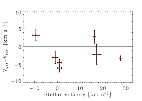
Figure 14: Velocity shifts $V_{\rm{gas}}$ - $V_{\rm{star}}$ as functions of $V_{\rm{star}}$. The gas velocity refers to the central velocity of the narrow component of the CO $\rm{v}=1-0$ lines.

The central velocities of the CO gas and stellar photosphere are compared to look for differences indicative of a wind or outflow, which could explain the narrow low velocity peak. The stellar radial velocities in Table 5 are taken from literature measurements of photospheric optical absorption lines. The photospheric absorption lines for our sample of sources are generally heavily veiled by continuum emission related to accretion, leading to uncertainties in the stellar velocity measurements of the order of 1-2 km s^-1.

The differences between the molecular gas radial velocity of the narrow component and the stellar radial velocity are small with shifts of $|V_{\rm{CO}}$ - $V_{\rm{star}}|$ $\lesssim$ 5 km s^-1, see Fig. 14. The shifts are more commonly seen towards the blue rather than the red, indicating that the CO gas is moving towards us relative to the star. However, the velocity shifts are only 1– 2$\sigma$ and may not be significant.

The small velocity differences rule out an origin of the lines in a fast moving disk wind or outflow. However it is still possible that the lines are emitted by gas in a slow disk wind. Najita et al. (2003) also do not see any significant velocity shifts between the radial velocity of the star and the gas within their few km s^-1 uncertainties.

4.2 Excitation temperatures

4.2.1 Rotational temperatures

The extracted fluxes of the ¹²CO $\rm{v}=1-0$ and ¹³CO lines are used to produce excitation diagrams and thus calculate the gas rotational temperatures. This calculation is done by using the Boltzmann distribution, which assumes that the excitation in the gas can be characterized by a single excitation temperature and that the emission is optically thin;

$$\frac{N_{i}}{g_{i}}=\frac{N_{\nu}}{Q_{r}(T_{\rm{rot}})}e^{-\frac{E_{i}}{kT_{\rm{rot}}}}$$ (1)

and where the column density $N_{i}$ of the upper level $i$ is described by,

$$N_{i}=\frac{4\pi F_{i}}{\Omega A_{ij}h\nu}$$ (2)

where the solid angle $\Omega$ = $D_{\rm em}$/${d^{2}}$ includes the emitting area $D_{\rm em}$ and the distance $d$ to the object. The other quantities are the Einstein coefficient $A_{ij}$ [s^-1], the frequency $\nu$ [cm^-1] and the measured line flux $F_{i}$ [W m^-2], the statistical weight $g_{i}$ of the upper level, the total column density $N_{\nu}$ for vibrational level $\rm{v}$, the excitation temperature $T_{\rm{ex}}$ and the rotational partition function $Q_{r}(T_{\rm{ex}})$. Plotting the upper energy levels $E_{i}$ against $\ell$n$(F_{i}$/$A_{ij}\nu{g}_{i})$ will give the rotational temperature $T_{\rm{rot}}$ by measuring the slope of the fitted line given by -1/$T_{\rm{rot}}$.

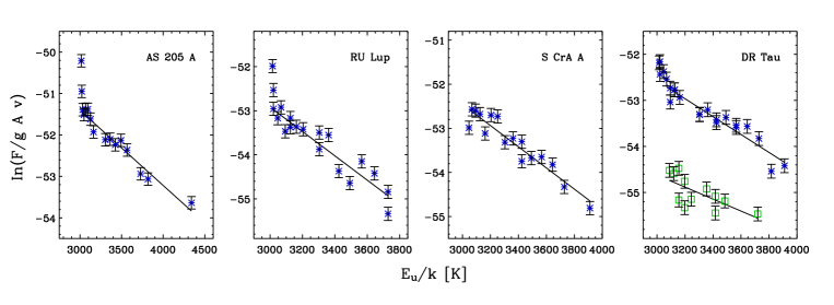
Figure 15: Rotational diagrams for T-Tauri stars AS 205 A, DR Tau, RU Lup and S CrA A. Blue stars represent ¹³CO lines and green squares C¹⁸O lines.

Table 7: Rotational temperatures $T_{\rm rot}$ derived from the ¹³CO lines, together with the vibrational temperatures $T_{\rm{vib}}$.

Source	$T_{\rm rot}$ [K]	$T_{\rm{vib}}[K]$
AS 205 A	550 $\pm$ 40	1740 $\pm$ 150
DR Tau	510 $\pm$ 40	1680 $\pm$ 140
RU Lup	360 $\pm$ 20	-
S CrA A	420 $\pm$ 30	1730 $\pm$ 140

The rotation diagrams for the ¹²CO lines are not linear, which suggests that the lines are optically thick. In addition, UV-pumping can cause non-linearity between the different transitions (Krotkov et al., 1980). To overcome this problem, rotational temperatures have been estimated using only the ¹³CO emission lines for the 4 sources, AS 205 A, DR Tau, RU Lup and S CrA A, for which sufficiently high $S/N$ emission lines are detected, see Fig. 15 and Table 7. The relative error of the line fluxes is taken to be 15% based on the noise in the spectra and uncertainties in the baseline fits. Only lines with $J_{u}>$1 are taken into account in the fit.

While ¹³CO is significantly less abundant than ¹²CO, ¹³CO lines may also be optically thick. ¹³CO lines with $\tau\approx$1 have, for example, been seen in the disk around Herbig star AB Aur by Blake & Boogert (2004). The inferred rotation temperatures of the 4 sources span 300–600 K, which is lower than 1100–1300 K found for the T Tauri sample of Najita et al. (2003) but within the temperature interval of 250–800 K given in Salyk et al. (2009). The discrepancy with Najita et al. (2003) may arise from differences in methodology. Najita et al. (2003) fit ¹²CO data covering lines with upper energies levels of up to 10⁴ K, which they assume to be optically thin. They performed a linear fitting based on this assumption, but curvature in their rotation diagrams indicates that their ¹²CO lines are likely also optically thick, leading to uncertainties in their extracted temperatures. Another explanation for the temperature difference may be the lack of higher $J$-transitions in our data set. However, AS 205 A includes ¹³CO transitions up to $E_{i}$ = 4400 K, and still has a lower temperature of 550 $\pm$ 40 K. The temperature estimates by Salyk et al. (2009) based on ¹²CO should be more reliable since they took optical depth effects into account. In addition, a rotational temperature of 770 $\pm$ 140 K has been estimated for DR Tau using the C¹⁸O lines, which is close to the temperature of 510 $\pm$ 40 K given by the ¹³CO lines (Fig. 15). If the two highest-$J$ ¹³CO lines are excluded from the fit, the ¹³CO rotational temperature increases to 610 $\pm$ 70 K, which is consistent with the C¹⁸O temperature within the error bars. These two high-$J$ ¹³CO lines are very weak and their fluxes may have been underestimated.

We determine the ¹³CO/C¹⁸O ratio for DR Tau to examine whether the ¹³CO emission is indeed optically thin. The ratio is calculated by comparing the fluxes in the R(5) and P(16) lines for ¹³CO with the R(5) and P(17) lines for C¹⁸O, chosen because they are not blended and have similar $J$. This gives ¹³CO/C¹⁸O = 6.3 $\pm$ 1.0 which is close to the overall abundance ratio of ¹³CO/C¹⁸O = 8.5 observed in the solar neighborhood (Wilson & Rood, 1994). The optical depth of ¹³CO is estimated to be $\tau$ = 0.3 $\pm$ 0.2. Inferred column densities and emitting areas will be presented in Brown et al. (in prep.), based on combined fits to the ¹²CO and ¹³CO lines.

4.2.2 Vibrational temperatures

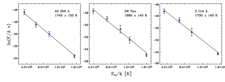
Figure 16: Vibrational diagrams for AS 205 A, DR Tau and S CrA A. Triangles represents upper limits.

Vibrational temperatures are determined for the three sources, AS 205 A, DR Tau and S CrA A, for which high $S/N$ ¹²CO data exist for several vibrational transitions (see Fig. 16). The vibrational temperatures are calculated using the same relation between the flux of the lines and the upper energy levels as presented in equations 1 and 2. The assumption made here is that every vibrational level has the same rotational temperature. The only difference is that $\ell$n$(F_{i}$/$A_{ij}\nu$) instead of $\ell$n$(F_{i}$/$A_{ij}\nu{g}_{i}$), is plotted vs the upper energy levels $E_{i}$ to extract the vibrational temperature $T_{\rm vib}$ since the statistical weights of the vibrational levels are the same. One clear line, close in $J$-level and without strong line overlap, is chosen per ro-vibrational level (CO $\rm{v}=1-0$, $\rm{v}=2-1$ etc.) to extract the line fluxes.

The inferred vibrational temperatures are 1740 $\pm$ 150 K for AS 205 A, 1680 $\pm$ 140 K for DR Tau and 1730 $\pm$ 140 K for S CrA A. The same fits have been done without including the ¹²CO $\rm{v}=1-0$ lines since the lines within this band can be more optically thick than those for the higher vibrational transitions. However, excluding the ¹²CO $\rm{v}=1-0$ lines does not significantly change the results within the uncertainties. The upper limits of the $\rm{v}=5-4$ flux have been estimated using $F$ = 1.065 $I_{peak}$ $\Delta V$, where the $\Delta V$ is taken to be the same as that of a CO $\rm{v}=3-2$ line and the amplitude $I_{peak}$ = 3$\sigma$/$bin^{-1/2}$, where the parameter $bin$ is the number of pixels within $\Delta V$ and $\sigma$ is the rms of a clean part of the spectrum where the line of interest is expected. The detection level is set to 3$\sigma$.

The vibrational temperatures of $\sim$1700 K are in general higher than the rotational temperatures derived from the ¹³CO lines of 300-600 K. The inferred temperatures can be compared to Brittain et al. (2007) who find a lower rotational excitation temperature of $\sim$200 K compared with a vibrational temperature of 5600 $\pm$ 800 K for the disk around the Herbig Ae star HD 141569. Similarly, van der Plas et al. (subm.) detect lower rotational temperatures of $\sim$1000 K relative to vibrational values of $\sim$6000 – 9000 K for three other Herbig Ae/Be stars. Both papers interpret the higher vibrational temperatures as caused by UV-pumping into the higher vibrational levels.

The results presented here indicate that UV-pumping may also be an important process for populating the higher vibrational levels in disks around T Tauri stars, especially for the broad-based single peaked sources. The rotation/vibration temperature differences in Brittain et al. (2007) and van der Plas et al. (subm.) are, however, much larger than those derived here. This may be due to the stronger UV fields from Herbig Ae/Be stars than T Tauri stars in the wavelength range where CO is UV-pumped.

Additional UV flux above the stellar photosphere can be produced by accretion (Valenti et al., 2000). Table 3 includes accretion luminosities taken from the literature for our T Tauri stars. These accretion luminosities are based on measurements of the hydrogen continua or H$\alpha$ line emission from the sources. The average accretion luminosity for those broad-based single peaked lines for which accretion luminosities have been measured, is 0.5 L_⊙. This value is higher than the average accretion luminosity of 0.1 L_⊙ which is calculated for the rest of the sample of disks that are shown in Table 3. The strong Pfund-$\beta$ lines observed in our data provide an additional confirmation of ongoing strong accretion (see Fig. 2). Higher accretion rates lead to higher UV fluxes, which, in turn, increase the UV pumping rate of CO into higher vibrational states. Quantitative estimates of the effect have been made by Brown et al. (in prep.) using the actual observed UV spectra for stars with spectral types A–K in an UV excitation model. Even if the enhanced UV from accretion for the T Tauri stars is included, however, the resulting vibrational excitation temperatures for a K-type star with additional UV due to accretion are still lower than those using an A-star spectrum. For the ${\rm v}=1-0$ emission, the question remains how much UV-fluorescence contributes relative to thermal excitation.

4.3 Lack of extended emission

Table 8: The upper limit on the projected radial extent $\Delta{R_{line}}$ of the line emission, together with $\Delta{R_{instr}}$.

Source	$\Delta{R_{instr}}$ [AU]	$\Delta{R_{line}}$ [AU]
AS 205 A	15.1 $\pm$ 0.1	$<$2.1
DR Tau	14.5 $\pm$ 0.1	$<$1.7
RU Lup	17.9 $\pm$ 0.2	$<$2.5
S CrA A	15.9 $\pm$ 0.2	$<$2.0
S CrA B	-	-
VV CrA Ab	16.6 $\pm$ 0.5	-
VW Cha	23.4 $\pm$ 2.3	$<$10.4
VZ Cha	20.7 $\pm$ 1.0	$<$6.3

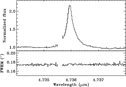
Figure 17: Top: The spectral line CO $\rm{v}=1-0$ P(8) for AS 205. Bottom: The FWHM of the spatial profile of the above spectrum at each individual wavelength point. No increase in FWHM is seen at the position of the line.

Figure 18: The stacked square root of the formal second moment $(\mu_{2})^{1/2}$ of the spectral trace for the ¹²CO emission lines. About 5–10 clean lines for each source were used for stacking. The square root of the second moment $(\mu_{2})^{1/2}$ is multiplied with * = 0.2 for sources with a larger uncertainty in the second moment. The vertical shift for respective source is: AS 205 A = 0 AU, DR Tau = -3.4 AU, RU Lup = -7.0 AU, S CrA A = -7.2 AU. For VW Cha and VZ Cha the shifts are 5.5 and 3.7 AU after multiplication with 0.2.

Information about the spatial extent of the CO emission from broad-based single peaked sources is an important ingredient for constraining models of their origin. The variance or formal second moment $\mu_{2}$ of the spectral trace is calculated at each wavelength from the 2-dimensional spectrum, according to the following equation.

$$\mu_{2}=\Sigma(x_{i}-C)^{2}\times F_{i}/\Sigma F_{i}$$ (3)

where $x_{i}$ is the spatial position, $F_{i}$ is the flux at that point and $C$ is the centroid position computed from $C=\Sigma x_{i}\times F_{i}/\Sigma F_{i}$.

For continuum emission, the average value of the second moment reflects the spatial resolution provided by the AO system, assuming that the continuum is not spatially extended. If the line emission is spatially extented, the values of $\mu_{2}$ will be larger than the noise in the continuum $\mu_{2}$ signal at wavelengths where the line emits. There is no significant detection of extended line emission for any of our sources, see Fig. 17 and Fig. 18. An upper limit on the radial extent of the line emission, $\Delta{R_{line}}$, is therefore calculated using the formula $\Delta{R_{line}}^{2}$ $\leq$ ($\Delta{R_{instr}}+\sigma_{\Delta R}$)² $-\Delta{R_{instr}}^{2}$, where $\Delta{R_{instr}^{2}}$ is equal to the mean of $\mu_{2}$/2 of the continuum and $\sigma_{\Delta R}$ is the standard deviation of ($\mu_{2}$/2)^1/2. The values listed in Table 8 include an additional correction factor (1 + $C/L$), where $C/L$ is the continuum/line flux ratio, because the total centroid is diluted by the continuum flux. These results show that most of the projected CO emission must originate from within a few AU for AS 205 A, DR Tau, RU Lup and S CrA A. S CrA B and VV CrA A (not shown) have a feature close to the central velocity of the line, however this can be explained by contamination from the companion star. The small feature seen for S CrA A may be a detection of extended line emission. VW Cha and VZ Cha have higher upper limits of the projected radial line extent of 10.4 and 6.3 AU respectively which is caused by a higher noise in the second moment of the continuum emission.

Since the position angle of the slit is arbitrary with respect to that of the disks in our observations, an additional check on the lack of radial extended emission is provided by the different spatial line profiles of the stacked CO $\rm{v}=1-0$ lines of AS 205 A, DR Tau and S CrA A taken at 3 different rotational angles. All three show exactly the same profile. This means that the CO emission originates from within a few AU at many different angles around the sources.

5 Discussion

Three possibilities for the origin of broad-based single peaked profiles are discussed below: a Keplerian rotating disk, a disk wind or a funnel flow.

5.1 Rotating disk

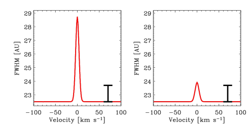
Figure 19: The second moment of the modeled spatial line profile for AS 205 (10 AU = 0$\aas@@fstack{\prime\prime}$08 at a distance of 125 pc). The model in the left plot includes extended emission out to 30 AU and $\Delta V_{\rm mod}$=3 km s^-1. The model in the right plot includes emission out to 10 AU and an increased $\Delta V_{\rm mod}$=7 km s^-1 (see Fig. 5). Error bars represent the 3$\sigma$ noise limit for AS 205 A in Fig. 18. Both models use the observed position angle of 115$\degr$ which is 50$\degr$ off from the position angle of 165$\degr$ of the AS 205 A disk (Andrews et al., 2009).

The results presented in $\S$3.2 show that broad-based single peaked lines (category C) cannot be reproduced using a Keplerian model with a power-law temperature profile. Increasing the local line broadening parameter $\Delta{V}_{\rm mod}$ to $\sim$8 km s^-1 removes the double peak, but a larger local line broadening is not sufficient to give a good fit between the disk model and the data. As seen in $\S$ 3.2.3 a Keplerian disk model can fit the data by solving for a temperature structure. The best fits have a plausible temperature structure but require extended emission, possibly in combination with an increase in the local broadening parameter.

The results of § 4.3 show that the bulk of the emission comes from within a few AU which means that a Keplerian model with a non-standard temperature profile including extended emission out to 30 AU cannot explain the broad-based single peaked line profiles. Even the model with enhanced turbulence and emission out to 10 AU becomes marginal, as illustrated by the expected second moments in these non-standard cases (Fig. 19). The vertical error bars in Fig. 19 represent the 3$\sigma$ noise limit in AU for AS 205 A. Similar results hold for most of the other sources, although the Keplerian models with a non-standard temperature profile including an enhanced turbulence cannot be fully ruled out for sources like VW Cha and VZ Cha for which the limits on the spatial extent are larger.

Carr et al. (2004) invoked a larger local line broadening of 7–15 km s^-1 in their disk models to obtain a better fit to CO $\rm{v}=2-0$ band head profiles observed toward various young stellar objects. As discussed in their paper, such values are much larger than the sound speed of a few km s^-1 in the inner disk, whereas models of turbulence in disks typically give velocities that are less than the sound speed (e.g., Klahr & Bodenheimer, 2006). In addition, these turbulent values are much higher than those inferred from observations of gas in the outer disk (Qi et al., 2006; Hughes et al., 2009), although the turbulence in a warm surface layer near the star may differ from that in the outer regions. A more extended discussion of turbulence in inner disks is given in Carr et al. (2004). Even though we cannot fully exclude an increased level of turbulence for some of our sources, this is unlikely to be the sole explanation for the broad-based single peaked line profiles observed here.

In summary, the above discussion shows that a pure Keplerian disk model does not fit the data. However, the estimated rotational temperatures of 300 to 800 K for the broad centrally peaked sources are consistent with the temperature expected for the inner parts of a disk. The symmetry of the lines and the small radial velocity shift between the gas and the star (a maximum of $\sim$5 km s^-1) are additional indications that the emission may originate in a disk. Therefore, it is likely that at least part of the emission originates from the disk but some additional process must contribute to these line profiles as well.

5.2 Disk wind

5.2.1 Thermally launched winds

Strong outflows are excluded due to the small velocity shifts of the molecular gas relative to the central star. Thermally launched winds are driven by irradiation of either FUV (far-ultraviolet), EUV (extreme ultraviolet), or X-ray photons (Alexander, 2008; Gorti & Hollenbach, 2009; Ercolano & Owen, subm.). Irradiation of the upper layers of the disk heats the gas to such high temperatures that the thermal energy exceeds the gravitational potential, leading to a flow off the disk surface. The launching radius is roughly given by $R_{g}$ = $GM_{\star}/V_{\rm{orb}}^{2}$, where $V_{\rm{orb}}$ is the orbital speed of the gas. The wind retains the Keplerian rotational velocity of the launch radius.

If the disk is illuminated by EUV radiation, an HII region forms in the upper layer of the disk atmosphere. The ionized gas reaches a temperature of 10⁴ K, which corresponds to $V$ $\sim$10 km s^-1. For a 1 $M_{\odot}$ star, the launching radius is then $R_{g}$$\sim 5-10$ AU, and the wind is launched with a velocity of $\sim 5-10$ km s^-1 (Alexander, 2008). This small velocity shift is consistent with the small velocity shifts we see in the CO gas emission relative to the stellar radial velocity. However, an EUV-driven wind consists mostly of ionized gas, so that CO may be photodissociated. Detailed models of the CO chemistry are needed to test whether enough CO can survive in such a wind to produce the observed CO line profiles.

In the X-ray and FUV photoevaporation models of Gorti & Hollenbach (2009), the evaporating gas is cooler than the EUV-irradiated gas. The expected launching radii of 10–50 AU for X-ray photoevaporation and $>$50 AU for FUV photoevaporation are inconsistent with the lack of spatially-extended emission in our CO spectra. However, in models of photoevaporation by soft X-ray emission by Ercolano & Owen (subm.), the launching radius is closer to the star. Ercolano & Owen (subm.) calculate profiles for atomic and ionized species within this model and predict symmetric, broad-based, single-peaked line profiles with small blueshifts of 0–5 km s^-1.

As for the EUV models, a detailed CO chemistry needs to be coupled with the wind model to test this scenario, but the fact that the wind is mostly neutral will help in maintaining some CO in the flow.

In summary, EUV and soft-X-ray photoevaporation of the disk might produce some CO emission at low velocities. More detailed studies of the CO chemistry and velocity fields in the thermally-launched wind are needed to determine where CO can survive in the wind and the resulting emission line profile.

5.2.2 Magnetically launched winds

Magnetic fields of Classical T Tauri stars exert torques that are thought to be strong enough to launch powerful winds. Edwards et al. (2006) describe two types of winds that are seen in absorption in the He 1 $\lambda 10830$ line, one with velocities of around 250 km s^-1 and another with lower speeds up to 50 km s^-1. These velocity shifts are also commonly observed in optical forbidden lines, such as [O I] 6300 Å. The high velocities are not consistent with the velocities seen in the broad-based single peaked CO emission, making this scenario highly unlikely.

5.3 Funnel flow

Accretion from the disk onto the star is thought to occur in a funnel flow along strong dipolar field lines (e.g., Hartmann et al., 1994; Bouvier et al., 2007; Yang et al., 2007; Gregory et al., 2008). Najita et al. (2003) rule out the possibility that the funnel flow could produce some CO emission because the temperatures in the funnel flow are expected to be $\sim 3000-6000$ K (Martin, 1997), higher than the measured temperatures of the CO-emitting gas. Models of observed hydrogen emission line profiles are consistent with these temperatures (Muzerolle et al., 2001; Kurosawa et al., 2006). However, Bary et al. (2008) suggest that the relative hydrogen emission line fluxes may also be consistent with cooler temperatures of $\sim 1000-1500$ K, and cooler temperatures may be present where the funnel flow connects with the disk. Najita et al. (2003) show that a modeled CO emission line profile from a funnel flow would have a double peaked line profile with no velocity shift (see Fig. 10b in their paper), which disagrees with the presence of the narrow emission peak seen in the line profiles discussed here. Thus, funnel flows are also not likely to be the origin of the observed emission.

6 Conclusions

Using CRIRES spectroscopy of CO ($\Delta\rm{v}=1$) ro-vibrational emission lines around 4.7 $\mu$m from a sample of 50 T Tauri stars, we find that the line profiles can be divided into three basic categories: A) narrow single peaked profiles, B), double peaked profiles and C) single peaked profiles with a narrow peak ($\sim 10-20\,\rm km\,s^{-1}$), but broad wings, sometimes extending out to 100 $\rm km\,s^{-1}$. The broad-based single peaked line profiles are rather common, since they were detected in 8 sources in a sample of about 50 T Tauri stars. These 8 sources have preferentially high accretion rates, show detections of higher vibrational emission lines (up to $v=4$) and have CO lines with unusually-high line-to-continuum ratios relative to all other sources within our sample. For at least one of the disks (S CrA B), the narrow component decreases faster for higher $J$ lines than the broad component, implying that the narrow component is colder. Generally, however, the two component fits give similar temperatures and central velocities.

The broad-based single peaked emission originates within a few AU of the star with gas temperatures of $\sim$300 – 800 K. The line profiles are symmetric and the gas radial velocity is close to the stellar radial velocity. These characteristics point toward an origin in a disk. However, unlike the CO profiles from other objects that are double-peaked or have only narrow peak, the broad-based single peaked line profiles could not be well fit using a Keplerian model with a power-law temperature profile. The fits are improved if a large turbulent width of $\sim 8$ km s^-1 is invoked, but the overall profile fit is still poor. Models with an unusual temperature distribution, perhaps with enhanced turbulence, provide a much better fit to the line profiles but require emission out to larger distances than observed. Thus, the hypothesis that this emission originates in a pure Keplerian disk needs to be questioned and an additional physical component needs to be considered.

Several other scenarios are also ruled out. FUV radiation-driven winds have a launching radius of $>50$ AU that is inconsistent with the lack of spatially-extended emission in our data. Magneto-centrifrugal winds are observed to have blueshifts of 50 – 250 km s^-1, which are inconsistent with the lack of a significant velocity shift in the symmetric CO emission lines. A funnel flow is also unlikely because emission near the inner rim of the disk should have a double-peaked line profile, and because the temperatures in the funnel flow are expected to be higher than the calculated CO rotational temperatures.

The most plausible explanation for the broad-based single-peaked line profiles is therefore some combination of emission from the warm surface layers of the inner disk, contributing to the broad component through Keplerian rotation, and a disk wind, responsible for the narrow component. A thermally launched disk wind, perhaps driven by EUV radiation or soft X-rays will have a small velocity shift of $\Delta{V}$ of 0-10 km s^-1, which is marginally consistent with the maximum detected velocity shift of $\Delta{V}\sim$5 km s^-1.

More information, including independent estimates of inclination angles, detailed models of CO chemistry and line profiles that originates in disk winds and the inner regions of disks, and spectro-astrometry of emission from these sources, is needed to distnguish the contributions from a disk (perhaps with enhanced turbulence) and a disk wind. These line profiles will be further discussed by Pontoppidan, Blake & Smette (subm.) using a combined disk and slow molecular disk wind model to analyze the spectro-astrometric data of these sources.