Variation of the extinction law in the Trifid nebula

Abstract

Context. In the past few years, the extinction law has been measured in the infrared wavelengths for various molecular clouds and different laws have been obtained.

Aims. In this paper we seek variations of the extinction law within the Trifid nebula region. Such variations would demonstrate a local dust evolution linked to variation of the environment parameters such as the density or the interstellar radiation field.

Methods. The extinction values, $A_{\lambda}/A_{V}$, are obtained using the 2MASS, UKIDSS and Spitzer/GLIMPSE surveys. The technique is to inter-calibrate color-excess maps from different wavelengths to derive the extinction law and to map the extinction in the Trifid region.

Results. We measured the extinction law at 3.6, 4.5, and 5.8 $\mu$m and we found a transition at $A_{V}\approx 20$ mag. Below this threshold the extinction law is as expected from models for $R_{V}=5.5$ whereas above 20 mag of visual extinction, it is flatter.Using these results the color-excess maps are converted into a composite extinction map of the Trifid nebula at a spatial resolution of 1 arcmin. A tridimensional analysis along the line-of-sight allowed us to estimate a distance of $2.7\pm 0.5$ kpc for the Trifid. The comparison of the extinction with the 1.25 mm emission suggests the millimeter emissivity is enhanced in the dense condensations of the cloud.

Conclusions. Our results suggest a dust transition at large extinction which has not been reported so far and dust emissivity variations.

1 Introduction

During the last three decades, dust evolution in the interstellar medium has been studied mostly through the grain emission in the far-infrared and then the sub-millimeter wavelengths. The analysis of the surface brightnesses at 60 and 100 $\mu$m observed by IRAS lead to distinguish a small and a big grain component where the small grains are the major contributor at 60 $\mu$m (Boulanger et al., 1988; Laureijs et al., 1991). The transition from small to big grains occurs at a typical visual extinction of 1 mag. More recently a new transition was discovered in the dust composition with the formation of fluffy grains. The analysis of PRONAOS sub-millimeter observations by Bernard et al. (1999) yielded to the discovery of a population of enhanced-emissivity dust grains which have a lower equilibrium temperature. This emissivity enhancement in the far-infrared by a factor of about 3 (Cambrésy et al., 2001) requires the existence of composite grains formed by the coagulation of small grains. A large scale study on the whole Galactic anticenter hemisphere showed this transition also occurs at low extinction, $A_{V}\approx 1$ mag (Cambrésy et al., 2005). It might be closely related to the recent discovery made by Molinari et al. (2010a) with Herschel data where this same density threshold seems to indicate the transition where diffuse clouds start to collapse into filaments.

With the wealth of available deep data in the near and mid-infrared it is now possible to investigate the interstellar grain properties at shorter wavelengths. In this spectral domain a lot of progresses has been made in the past few years through the study of the extinction law. Dense clouds can be probed on large scales and for various astrophysical environments. Recent studies with Spitzer data (Indebetouw et al., 2005; Flaherty et al., 2007; Román-Zúñiga et al., 2007; Chapman et al., 2009) focused on different clouds and obtained different extinction laws. We propose in this work to look for possible variations of the extinction curve within a single cloud. We choose an active star-forming region which includes the famous HII region M20, the Trifid nebula. Its location in the Galactic plane at only 7 degrees from the Galactic center offers a high stellar density which is ideal to probe the extinction distribution. The distance of this young nebula ($10^{5}$ years) is still debated. The observation of the central O7 star responsible for the photoionization, HD 164492, yields a distance from 1.67 kpc (Lynds et al., 1985) to 2.8 kpc (Kohoutek et al., 1999). This active region has its first generation of massive stars interacting with the interstellar medium and is very likely triggering a second generation of star formation (Cernicharo et al., 1998). The state-of-the-art for the Trifid star-forming region is presented in a review paper by Rho et al. (2008).

The extinction law is generally estimated in molecular clouds as a whole and the discrepancies between the different results are interpreted as variations of the dust optical properties from cloud-to-cloud due to the environment. Obviously variations should also be observed within molecular clouds. As the density increases from the envelope to the core of a cloud, the dust properties, hence the extinction law, should be affected. An attempt to detect such a variation was proposed by Román-Zúñiga et al. (2007) in their study of a dark cloud core, B59, up to $A_{V}\approx 59$ mag but they did not succeed. Olofsson & Olofsson (2010) used five different methods to derive the extinction law in B335. The scatter in their result was consistent with the uncertainties so they could not conclude on any evolution of the extinction law within the cloud. Chapman et al. (2009) managed to find variations by averaging their result from several clouds and they showed evidence for grain growth at $A_{K_{s}}>1$ mag ($A_{V}>9$). A global galactocentric variation of the extinction law has also been reported by Zasowski et al. (2009) in a large scale study that excluded molecular clouds.

The present study focuses on the variations of the extinction law within the molecular cloud associated with the Trifid nebula. Our analysis relies on the 2MASS (Skrutskie et al., 2006), UKIDSS (Lawrence et al., 2007) and GLIMPSE II (Churchwell et al., 2009) surveys. Special attention is given to the data filtering to limit the possible biases as explained in Sect. 2. Our original method to derive the extinction law from 3.6 to 5.8 $\mu$m is based on the color mapping rather than the classical analysis of the source list distribution in a color-color diagram. The details and the advantages of this technique are presented in Sect. 3 while Sect. 4 describes the final extinction map making and a tridimensional analysis of the Trifid line-of-sight which allows us to disentangle the complexity of this direction. In addition we studied the dust emissivity at 1.25 mm by comparing the masses derived from the dust continuum emission and the dust absorption. We conclude in Sect. 5.

2 Data preparation

2.1 Datasets

Our study covers a large field of $1.6^{\circ}\times 1.4^{\circ}$. The 2MASS near-infrared data provides $JHK_{s}$ fluxes for the whole sky. The high stellar density in the Trifid direction induces a loss of sensitivity as 2MASS sources with less than 5″ separation are affected by confusion. The degradation reaches almost 1.5 mag in each filter, with completeness level of only 12.8 mag for the $K_{s}$ band for instance.

Deeper $JHK_{s}$ fluxes are obtained from the UKIDSS 6th data release (UKIDSSDR6plus) of the Galactic Plane survey. UKIDSS uses the UKIRT Wide Field Camera (WFCAM; Casali et al., 2007). The photometric system is described in Hewett et al. (2006), and the calibration is described in Hodgkin et al. (2009). The pipeline processing and science archive are described in Hambly et al. (2008).

Longer wavelengths from Spitzer/IRAC are publicly available through the GLIMPSE II legacy survey. We used the high reliability point source Catalog (v2.1) which includes data from epochs 1 and 2.

The merged catalog between 2MASS, UKIDSS and GLIMPSE tables results from a 1″ cone search. Completeness limit magnitudes for all filters are presented in Table 1. For bright stars, the 2MASS photometry is chosen over the UKIDSS photometry which is affected by saturation. Although the UKIDSS photometry is directly calibrated on 2MASS we found a systematic difference between the two systems:

$$\begin{array}[]{lll}J\mbox{(2MASS)}&=J\mbox{(UKIDSS)}&+0.084\\ H\mbox{(2MASS)}&=H\mbox{(UKIDSS)}&-0.074\\ K_{s}\mbox{(2MASS)}&=K_{s}\mbox{(UKIDSS)}&-0.003\end{array}$$

We corrected the UKIDSS photometry to match the 2MASS system. The UKIDSS astrometry has also been corrected to match the GLIMPSE positions by adding 0.12 and 0.07 arcsec to the right ascension and declination, respectively. In the following, only magnitude measurements with an uncertainty smaller than 0.15 mag will be considered. It yields about $2\times 10^{5}$ sources at $K_{s}$, $6\times 10^{5}$ at 3.6 $\mu$m in the range $\mbox{R.A.}\in[269.50,271.29]$ and $\mbox{Dec.}\in[-23.6,-22.2]$.

Table 1: Completeness limit magnitudes. For UKIDSS the luminosity function slopes are not well defined, so the peak values of the function for sources with an error smaller than 0.15 mag are displayed.

	2MASS	UKIDSS	UKIDSS(peak)	GLIMPSE
$J$	14.4	16.2	17.8
$H$	13.5	15.0	16.7
$K_{s}$	12.8	14.2	16.0
$[3.6]$				13.5
$[4.5]$				13.4
$[5.8]$				12.2
$[8.0]$				11.4

2.2 Source selection criteria

The analysis of the stellar color excess to investigate the cloud properties requires all stars to be background stars. The contamination by foreground objects cannot be neglected for the Trifid nebula located between 1.7 and 2.8 kpc probably in the Scutum Arm, behind the Sagittarius Arm. The procedure to remove foreground stars is statistical for two reasons: 1) the number of detected sources is close to $6\times 10^{5}$, and 2) there is a degeneracy between intrinsically red foreground objects and blue background sources. A color criteria would therefore be inefficient. It would actually lead to a source spatial distribution correlated with the dust distribution which is not consistent with the supposedly foreground nature of the stars. The individual identification is generally impossible, except in the high extinction region where the degeneracy can be raised. Keeping these constraints in mind, we choose a two steps strategy, first purely statistical and then individual and manual.

The statistical step consists in sampling the source catalog into a data cube with two spatial dimensions and a third dimension being a color axis. Only one star per box is allowed. Basically, stars are sampled by a 4 arcmin grid step according to their celestial coordinates and the third axis allows to color-sort the stars within a same 16 arcmin² pixel so that there is only a single star per 3D-box. The first slice of the cube represents a map where each pixel contains the color of the bluest object of the stack. The following slices contain redder and redder color values. The completeness limit of UKIDSS being not well defined we use only 2MASS and GLIMPSE for this statistical procedure. The variation of the stellar density makes the number of stars per pixel, and therefore the size of the stack, range from 85 to 387. For a 16 arcmin² pixel, it means the source density varies from $19\times 10^{3}$ to $87\times 10^{3}$ deg^-2. Once the cube is built, each plane from the bluest to the reddest is compared to a raw color map of the field, i.e. a non-calibrated extinction map. A correlation with the color map starts at the 38^th slice, meaning the distribution of the $\sim$38 bluest stars in all the 16 arcmin² pixels is not correlated with the dust distribution. They must be considered as foreground objects and the first 38 stars of each pixel, i.e. 8600 stars deg^-2, are thus removed from the original catalog. It represents from 10% to 45% of the sources detected at $K_{s}$ and $[3.6]$ depending on the position, i.e. the local source density.

At this point, only a fraction of the foreground stars is removed. A second step is required to filter the catalog in the regions where the contamination is critical because the foreground objects may even be the dominant population. Fortunately, in these regions the color degeneracy is raised by the strong reddening from the dust grains. To define these regions we build a [3.6]-[4.5] color map following the adaptive method described in Sect. 3.1.1. Then we select the pixels where [3.6]-[4.5]$>$0.35 mag ($A_{V}\approx 30$ mag) which yields a 25 arcmin² surface area. Such a high threshold guaranty the degeneracy with the intrinsic star color is broken. For this manual operation the restriction on UKIDSS data can be waived and $\sim$$10^{3}$ sources are detected in the 25 arcmin area at both $K_{s}$ and 3.6 $\mu$m with error smaller than 0.15 mag. The spectral energy distribution from 1.25 $\mu$m to 8 $\mu$m is examined for these sources. For each foreground star candidate, a color-composite $JHK_{s}$ image is built to compare the color of the candidate itself with the color of the surrounding objects. This visual inspection allows to make the final classification of the source since a foreground star appears bluer than the surrounding objects. Among the $\sim$$10^{3}$ sources detected at $K_{s}$ and 3.6 $\mu$m, 20% are classified as foreground stars. It corresponds to a total foreground star density of $\sim$$37\times 10^{3}$ deg^-2. It worth noting that for sources together detected at $J$, $H$ and $K_{s}$ instead, the contamination level in the 25 arcmin² reaches 55%. This is because many background stars are lost when the $J$ detection is required.

Beside the foreground stars, there is a contamination by the Young Stellar Objects (YSOs) that are formed in the molecular cloud associated with the Trifid nebula. Several studies, at various wavelengths, provide us with a source list of YSOs that we removed from our catalog. The most important contribution is from Rho et al. (2006) who analyzed the infrared colors from Spitzer IRAC and MIPS data. It yielded the identification of 161 YSOs (37 class I/O, 13 hot excess, 111 class II). Previous studies of the young star population in the Trifid nebula used 2MASS, ASCA, ROSAT (Rho et al., 2001) and Chandra (Rho et al., 2004).

Finally, another possible contamination would be extragalactic sources. This effect is negligible based on the location of the Trifid nebula in the Galactic plane and close to the Galactic Center direction.

3 Extinction law

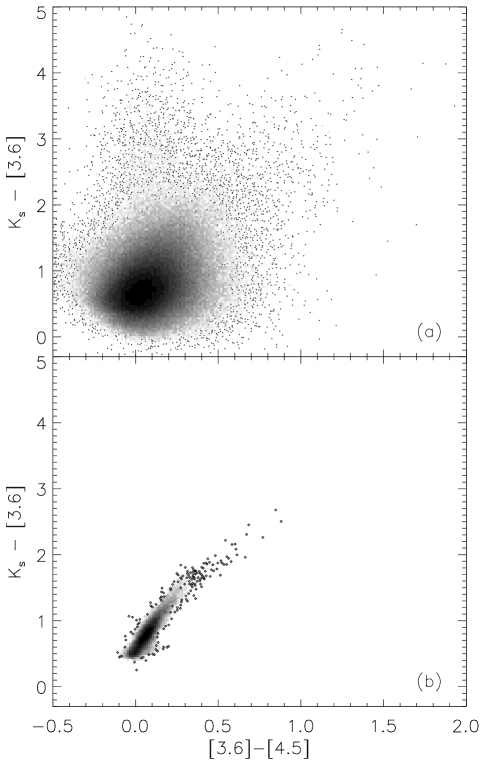
Figure 1: (a) Color-color diagram for stars with uncertainty smaller than 0.15 mag in the 3 bands. (b) Color-color diagram obtained using color maps instead of the source list. The exact same stars are used for both plots. The gray scale represents the density of the data points in the plot and the dots show the individual data points for low density.

The general idea of the method to derive the extinction law is trivial. It requires the knowledge of the relative extinction in two wavelengths, $A_{\lambda 1}/A_{V}$ $A_{\lambda 2}/A_{V}$, to evaluate the extinction at a third wavelength by measuring the slope of the star color distribution within a color-color plot $m_{\lambda 1}-m_{\lambda 2}/m_{\lambda 2}-m_{\lambda 3}$. The color-color diagram slope being equal to the color-excess ratio $E_{\lambda 1-\lambda 2}/E_{\lambda 2-\lambda 3}$ the value of $A_{\lambda 3}/A_{V}$ is inferred. Practically, this procedure is not necessarily that simple because of the scatter in the color-color diagram. The selection of a sub-sample as clean as possible is strongly recommended. Fig. 1a is restricted to sources with an uncertainty smaller than 0.15 mag at $K_{s}$, 3.6 and 4.5 $\mu$m although a large scatter is still present in the plot. In particular, the vertical elongation for $[3.6]-[4.5]\approx 0$ and $K_{S}-[3.6]>2$ is not real. It is due to a severe underestimation of the UKIDSS $K_{s}$ uncertainty for some sources. Fortunately, the method presented in the next section makes their contribution negligible because of their random spatial distribution.

Fig. 1 and several others in this paper represent plots as density maps for clarity reason. Dark means high density. Unless specified otherwise the overlaid symbols simply help to visualize the lowest density pixels that are hardly visible.

3.1 Color map making

3.1.1 Method

Although a slope could be measured in Fig. 1a, the scatter is large. The Trifid line-of-sight crosses various interstellar medium environments and all kind of stellar populations. This diversity, the high stellar density, and the relatively large distance of M20 make our goals more difficult to reach than for nearby molecular clouds such as Chamaeleon, Taurus or Rho Ophiuchus.

We propose a method based on the color maps that spectacularly improves the accuracy of the analysis. Fig. 1b was built using the exact same sources as Fig. 1a and both figures have the same axis, same scale. While each point in Fig. 1a corresponds to a single source, points in Fig. 1b actually represent individual pixels taken from two color maps, one for each axis. Using the color allows us to keep the same axis as in Fig. 1a but it is obviously equivalent to an extinction map assuming an extinction law. The impressive difference between the two figures highlights the superiority of using maps rather than a source list directly. Using maps permits to average the color of several individual nearby sources, and thus to reduce the scatter. Different methods are available to build an extinction map. Star count methods are sometimes used on large scale and for moderate extinction (Cambrésy, 1999; Dobashi et al., 2005). This approach is definitely not adapted to a highly obscured distant cloud in the Galactic plane. Too sensitive to the foreground star contamination the map would be noisy and seriously biased. Color-excess methods are better adapted. The first statistical method to map the extinction from color excess, called NICE, was proposed by Lada et al. (1994). Improvement were proposed and called NICER (Lombardi & Alves, 2001) and then NICEST (Lombardi, 2009). A variant technique from Cambrésy et al. (2002) proposes to replace the arithmetic mean color by the median color in cells and to fix the number of sources within a cell rather than its size. The latter step makes the method adaptive since the spatial resolution is always optimal, adjusted to the local density. A final convolution can be applied if a fixed spatial resolution is wished. This convolution minimizes a bias that would result in an underestimation of the extinction, compared to the usage of larger cells already at the final resolution size. Moreover the median is a powerful tool to limit the effect of the residual contamination by foreground stars and young stellar objects as detailed in Cambrésy et al. (2002).

All the color maps built for this work use the median color and follow the adaptive cell scheme with a fixed number of 3 stars per cell. The variable cell spatial resolution being $r_{i}$, a convolution by a Gaussian kernel of $\sqrt{1-r_{i}^{2}}$ arcmin is applied to reach a final resolution of 1 arcmin over the whole map.

3.1.2 Selection bias

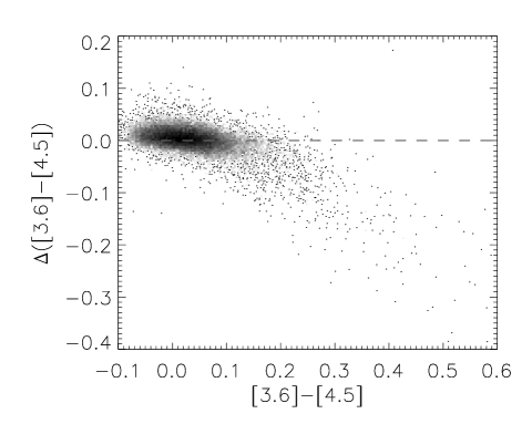
Figure 2: $[3.6]-[4.5]$ color difference from sources detected simultaneously in two different sets of 3 filters, $K_{s}({\rm 2MASS})/[3.6]/[4.5]$ and $[3.6]/[4.5]/[5.8]$, versus color.

Once a clean star sample is produced, i.e. filtered from foreground stars, YSOs and noisy photometry sources, the color maps are still subject to a selection bias. While it is mandatory to keep sources detected in all 3 bands to plot Fig. 1a, the Fig. 1b needs two color maps that can be built independently with only a 2 band detection criteria for each of them. Fig. 2 illustrates the color bias for $[3.6]-[4.5]$ when it is obtained from two different sets of 3 band detection criteria, $K_{s}/[3.6]/[4.5]$ or $[3.6]/[4.5]/[5.8]$. To exaggerate the effect $K_{s}$ is taken from 2MASS which is not as deep as UKIDSS. The $[3.6]-[4.5]$ average color is affected by the $K_{s}$ detection criterion which makes the color bluer, and by the [5.8] detection criterion which tends to select redder objects. It is not a simple offset as shown in Fig. 2 because this effect is more important for redder color. In terms of extinction, taking sources detected in the 3 bluer wavelengths yields an underestimation of the extinction. Using deeper $K_{s}$ data would obviously help since more sources detected at [3.6] and [4.5] would also be seen at $K_{s}$. However the effect cannot be avoided at large extinction because the $K_{s}$ band suffer from twice the extinction than at [3.6].

It is therefore critical to compare only maps that are built with the exact same sample of stars. It implies the $[3.6]-[4.5]$ color map needs to be built from a source list which contains stars detected in the 3 bands $K_{s}$, [3.6] and [4.5] if it is compared to a $K_{s}-[3.6]$ map, or from a source list which contains stars detected at [3.6], [4.5] and [5.8] if it is compared to a $[4.5]-[5.8]$ map.

A total of 6 color maps are built for our study: $H-K_{s}$, $K_{s}-[3.6]$, $[3.6]-[4.5]$, $[4.5]-[5.8]$. Each map is obtained with sources detected in 3 bands at the same time. There are 2 versions for the $K_{s}-[3.6]$ map and the $[3.6]-[4.5]$ map because the third band can either be the bluer or the redder one.

3.2 Results

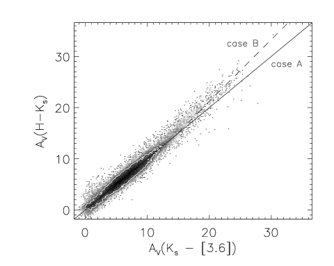
Figure 3: Extinction from $H-K_{s}$ color excess versus extinction from $K_{s}-[3.6]$ color excess. By adjusting $K_{s}-[3.6]$ to obtain a one-to-one regression line (solid line) we find $A_{[3.6]}/A_{K_{s}}=0.611$. The white iso-density contour delineates the region used to compute de regression line. The dashed line is the regression line for $A_{V}>20$ mag, it indicates the deviation at large extinction. Case A and B refer to Table 2.

Although the extinction law has been for long considered as universal in the infrared it is now admitted there are variations at wavelength longer than 2 $\mu$m. The spectral range that is pseudo-universal is actually restricted to 1-2 $\mu$m where the extinction is independent or very little dependent of the environment, i.e. dust temperature and density. Consequently, $A_{H}/A_{V}=0.175$ and $A_{K_{s}}/A_{V}=0.112$ (Rieke & Lebofsky, 1985) are assumed constant. It corresponds to $\beta=1.7$ in the expression $A_{\lambda}\propto\lambda^{-\beta}$ that is often used to describe the near-infrared extinction law. Values from 1.6 to 1.8 being reasonable, the effect of such a systematic uncertainty is discussed further in this section. The $H-K_{s}$ map can be converted into an extinction map using

$$A_{V}=\frac{(H-K_{s})-(H-K_{s})_{0}}{A_{H}/A_{V}-A_{K_{s}}/A_{V}}=15.87\;E_{H-K_{s}}$$

The extinction law is normalized to $A_{V}$ mainly for historical reason but it is more convenient to normalize to $K_{s}$. The relation between the extinction and the color excess becomes $A_{K_{s}}=1.78\;E_{H-K_{s}}$. The reference color $(H-K_{s})_{0}=0.54$ mag is estimated from the area with the smallest values within the map, about 50 arcmin south-west from the densest core of the cloud. This is much redder than the intrinsic stellar color because it includes the diffuse extinction along the line-of-sight. The reference color is relevant to provide an absolute extinction for the Trifid alone and it is discussed in the Sect. 4.2. It has absolutely no effect on the extinction law estimation nor on the relative extinction comparison from different parts of the field.

Fig. 3 represents $A_{V}$ from $H-K_{s}$ versus $A_{V}$ from $K_{s}-[3.6]$. Since $A_{V}=A_{K_{s}}/0.112$ is assumed, and by definition $A_{K_{s}}=E_{K_{s}-[3.6]}/(1-A_{[3.6]/A_{K_{s}}})$, the only free parameter to adjust to obtain a slope of 1 is the value of $A_{[3.6]}/A_{K_{s}}$. After the adjustment, it yields the value of $A_{[3.6]}/A_{K_{s}}=0.611$. Fig. 3 is presented as a density map for clarity and also because the density information is taken into account in the fitting process to exclude the low density pixels. Basically the minimum density level is fixed to 20% of the maximum density in the map. The color-coding used in the density plots is in log-scale so the 20% always corresponds to the dark region. The white iso-density contour delineates the region selected to compute the regression line in Fig.3. Any outlier is therefore fully eliminated with this technique.

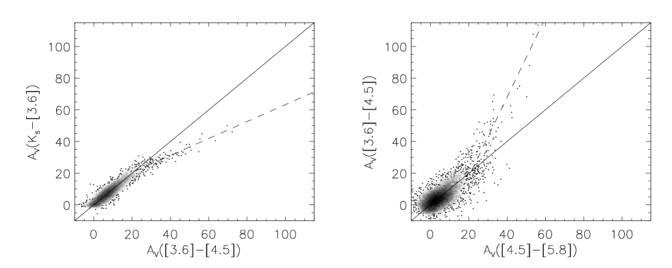
Figure 4: Each plot represents the extinction correlation from two different color excesses. The two parameters $A_{[4.5]}/A_{K_{s}}=0.500$ (left plot) and $A_{[5.8]}/A_{K_{s}}=0.398$ (right plot) are adjusted to obtain a one-to-one regression line (solid line). The dashed lines trace the deviation at large extinction, the corresponding slopes in these plots are $0.55\pm 0.02$ and $2.52\pm 0.09$, respectively.

Once $A_{[3.6]}/A_{K_{s}}$ is determined, $A_{[4.5]}/A_{K_{s}}$ is evaluated with a plot of $A_{V}$ from $K_{s}-[3.6]$ versus $A_{V}$ from $[3.6]-[4.5]$. A third similar plot will then provide $A_{[5.8]}/A_{K_{s}}$ (see Fig. 4). The results are $A_{[4.5]}/A_{K_{s}}=0.500$ and $A_{[5.8]}/A_{K_{s}}=0.398$.

Since the pixels falling in the low density regions of the $A_{V}$ vs. $A_{V}$ plot are ignored the fitting is performed on regions where the visual extinction is roughly smaller than 15 mag. At large extinction a striking deviation of the slopes is observed and outlined by the dashed lines in Figs. 3 and 4. The changes of slope occur at $A_{V}\approx 20$ mag ($A_{K_{s}}\approx 2.2$) and suggests a transition phase in the dust grain population. At such a high column density this result is unexpected. Contrary to studies in the far-infrared wavelengths which rely on the dust emission, there is no temperature degeneracy issue since it is based on stellar color mapping. A drawback of this technique is its limitation to the near-infrared spectral range. At wavelengths longer than $\sim$5 $\mu$m the number of detected stars is too low to have an acceptable spatial sampling of the molecular clouds while shorter wavelengths are so sensitive to the extinction that the cloud dense regions become totally opaque. A direct consequence on this limitation is that no evidence for a slope change can be seen in a $J-H$ vs. $H-K_{s}$ diagram because the visual extinction cannot go deeper than $\sim$20 mag with $J-H$. That prevents any conclusion on the extinction law variation at shorter wavelengths than 3.6 $\mu$m.

Table 2: Color excess ratios and resulting extinction law parameters. The two rows for $A_{V}>20$ mag represent different cases for $A_{[3.6]}/A_{K_{s}}$: case A propagates the same value as for small extinction, case B takes the actual measured value. We assume the power-law index $\beta=1.7$ (i.e. $A_{H}/A_{K_{s}}=1.563$) and results for $\beta=1.6$ and 1.8 are provided for case B. The main results from the literature for dense interstellar medium directions and from a dust model are indicated for comparison.

	$E_{H-K_{s}}/E_{K_{s}-[3.6]}$	$E_{K_{s}-[3.6]}/E_{[3.6]-[4.5]}$	$E_{[3.6]-[4.5]}/E_{[4.5]-[5.8]}$	$A_{H}/A_{K_{s}}$	$A_{[3.6]}/A_{K_{s}}$	$A_{[4.5]}/A_{K_{s}}$	$A_{[5.8]}/A_{K_{s}}$
$A_{V}<15$	$1.446\pm 0.002$	$3.508\pm 0.011$	$1.087\pm 0.007$	1.563	$0.611\pm 0.002$	$0.500\pm 0.003$	$0.398\pm 0.005$
$A_{V}>20$
case A	$1.446\pm 0.002$	$1.915\pm 0.018$	$1.496\pm 0.089$	1.563	$0.611\pm 0.002$	$0.408\pm 0.003$	$0.272\pm 0.011$
case B	$1.749\pm 0.003$	$2.317\pm 0.027$	$1.810\pm 0.091$	1.563	$0.678\pm 0.006$	$0.540\pm 0.003$	$0.463\pm 0.007$
case B, $\beta=1.6$				1.520	$0.703\pm 0.005$	$0.573\pm 0.003$	$0.500\pm 0.007$
case B, $\beta=1.8$				1.601	$0.656\pm 0.006$	$0.507\pm 0.003$	$0.424\pm 0.007$
Román-Zúñiga et al. (2007) for Barnard 59				1.55	$0.619\pm 0.029$	$0.512\pm 0.022$	$0.459\pm 0.024$
Flaherty at al. (2007) for Orion				1.55	$0.636\pm 0.003$	$0.540\pm 0.003$	$0.504\pm 0.003$
Chapman et al. (2009) for Ophiuchus, Perseus and Serpens				1.52	$0.640\pm 0.030$	$0.530\pm 0.030$	$0.460\pm 0.030$
Weingartner &Draine (2001) with $R_{V}=3.1$					0.40	0.25	0.17
Weingartner &Draine (2001) with $R_{V}=5.5$					0.60	0.49	0.40

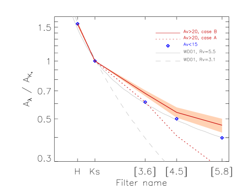
Figure 5: Extinction law. The two red lines corresponds to the cases described in Table 2 for $A_{V}>20$ mag. The shaded area indicates the systematic error, for case B only, resulting from $A_{H}/A_{K_{s}}$ uncertainty which can range from 1.52 ($\beta=1.6$) to 1.60 ($\beta=1.8$). At longer wavelengths than $K_{s}$, $\beta=1.6$ gives larger $A_{\lambda}/A_{K_{s}}$. Diamonds are for $A_{V}<15$ mag. The Weingartner & Draine (2001) model is plotted in gray with dashed and plain lines for $R_{V}=3.1$ and $R_{V}=5.5$, respectively. The axis scale is linear for $x$ and logarithmic for $y$.

Table 2 summarizes the results obtained from the slope measured in both Figs. 3 and 4. We consider two different cases for $A_{[3.6]}/A_{K_{s}}$ at $A_{V}>20$ mag:

• case A: $A_{[3.6]}/A_{K_{s}}=0.611$ is independent from the extinction, the value remains identical than at lower extinction (solid line in Fig. 3).

• case B: $A_{[3.6]}/A_{K_{s}}=0.678$ which is the value actually obtained from the slope of the dashed line in Fig. 3.

The statistical errors on the slope estimations are small and so are the errors on the computed $A_{\lambda}/A_{K_{s}}$. The systematic error on $A_{H}/A_{K_{s}}$ is the major source of uncertainty. We assume a value of 1.563 which corresponds to a power-law index of $\beta=1.7$ for the extinction law. Our results from Table 2 are plotted in Fig. 5. The shaded area delineates the systematic uncertainty for $\beta$ varying from 1.6 to 1.8. Using $\beta=1.6$, such as in Chapman et al. (2009), increases $A_{\lambda}/A_{K_{s}}$ to the upper border of the shaded area. Nishiyama et al. (2006) reported a higher value of $\beta=1.99$ which is not compatible with our observations. The Weingartner & Draine (2001) (hereafter WD01) model is overlaid for comparison. The variations in the extinction law found in this work are rather small compared to the dust evolution from $R_{V}=3.1$ to $R_{V}=5.5$. The variation being observed at visual extinction larger than 20 mag is likely the main reason for this dust transition to be unknown. In case A the extinction parameters at 4.5 and 5.8 $\mu$m are smaller at large extinction than at small extinction which is not realistic according the WD01 model. This case teaches us the small deviation observed in Fig. 3 cannot be ignored as it would make longer wavelength results inconsistent. Case B is more likely even if it yields a larger value than reported in the literature until now. The largest value prior to this work was from Chapman et al. (2009) with $A_{[3.6]}/A_{K_{s}}=0.64$. However their numbers are overestimated compared to ours or to Flaherty et al. (2007) because they chose a smaller $\beta$. Their results come from an average for Ophiuchus, Perseus and the Serpens molecular clouds which all form low-mass stars whereas the cloud associated with the Trifid is clearly more massive and forms OB stars. Flaherty et al. (2007) investigate the high-mass star-forming region of Orion and obtain a similar number of $0.636\pm 0.003$, significantly below our $A_{[3.6]}/A_{K_{s}}=0.678\pm 0.006$. They did find smaller values at all wavelengths in low-mass star-forming regions. The presence of massive star, in addition to a high density, may therefore be relevant.

WD01 attribute the variation of the extinction law with $R_{V}$ to grain growth only, although ice mantles onto dust grains contribute to the optical property variations. The main ice features relevant to our study originate from H₂O and CO₂ ices with absorption at 3.0 $\mu$m and 4.27 $\mu$m, respectively. Both H₂O and CO₂ ices are detected at visual extinction below 4 mag (Whittet et al., 2001; Bergin et al., 2005) where the WD01 model is still valid. This indicates ice is not sufficient to significantly modify the extinction law in the Spitzer/IRAC filters. We can also rule out the possibility that ice features saturate at $A_{V}\approx 20$ mag because they are observed at larger extinction without any saturation (A. Boogert, private communication). An example of spectrum is presented in Whittet et al. (1998, Fig.1) for a star with $A_{V}=21$ mag. It worth noting the H₂O ice band at 3.0 $\mu$m peaks outside the [3.6] IRAC filter (3.2-3.9 $\mu$m). Beside the absorption features, ice mantles make the grains more sticky, helping the coagulation process. Using Spitzer/IRS spectra McClure (2009) found evidence for a flattening of the extinction law at $A_{K}>1$ mag which would be due to the coagulation of ice-mantled grains. This suggests ice makes the coagulation process more efficient but it is not the dominant parameter since the coagulation starts well after ice-mantles appear. The abrupt change in the extinction law at $A_{V}\approx 20$ is not understood and we can only speculate that the high density in the Trifid cloud might allow a new structuring of the dust grains or that the shocks observed in the Trifid cloud could be determinant. In a recent work Boogert et al. (submitted to ApJ) also reported a flatter extinction law than WD01 based on a spectrum from 3 to 24 $\mu$m for a star with 25 mag of visual extinction.

4 From color to extinction

4.1 Composite map

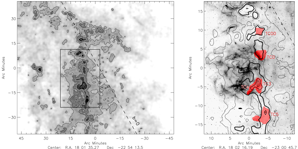
Figure 6: Left: large scale extinction map of the Trifid region. Right: GLIMPSE 8 $\mu$m image of the Trifid nebula with iso-extinction contours. In both figures contours correspond to $A_{V}=[10,15,20,40,60]$ mag, the dashed line follows the Galactic plane. The red shaded regions delineate the $S_{1.25}>10$ mJy/11” beam Trifid Condensations (TC, Cernicharo et al., 1998) studied in Sect. 4.3 at a 1 arcmin resolution.

The extinction law parameters derived in the previous section allow us to convert the color maps into extinction. To proceed we follow the more realistic case B for $A_{\lambda}/A_{K_{s}}$ when $A_{V}>20$ mag (see Table 2) and a reference color of $H-K_{s}=0.54$ mag. The associated zero points derived for the other colors are $K_{s}-[3.6]=0.497$, $[3.6]-[4.5]=-0.017$ and $[4.5]-[5.8]=0.187$ mag. The sensitivity of each map relies on the wavelengths used to build the color maps. Shorter wavelengths are more sensitive too smaller extinctions. The final extinction map presented in Fig. 6 is a combination defined as follow:

$$A_{V}\mbox{ from }\left\{\begin{array}[]{crll}&K_{s}-[3.6]&\mbox{ if }&A_{V}<15\mbox{ mag}\\ &[3.6]-[4.5]&\mbox{ if }&10<A_{V}<80\mbox{ mag}\\ &[4.5]-[5.8]&\mbox{ if }&A_{V}>60\mbox{ mag}\end{array}\right.$$

The transition between two maps is progressive and linear within the overlapping extinction ranges. A maximum visual extinction of $\sim$80 mag is reached. In complement to the extinction map Fig. 6 shows a close-up on the Trifid nebula observed at 8 $\mu$m with the iso-extinction contours superimposed. The parent molecular cloud is an elongated structure with its densest region lying just West of the famous optical nebula.

4.2 Tridimensional analysis, distance estimation

The extinction estimation relies on background stars. The meaning of background is not that trivial in the direction of the Trifid nebula since the line-of-sight crosses the whole galactic disk at only 1 kpc of the Galactic center. The complexity of the line-of-sight and the distance of the stars used for the analysis are critical and can change our interpretation of the color maps. Even the distance of the nebula is still uncertain. To address these issues we performed a tridimensional analysis which aims to separate the different components along the line-of-sight.

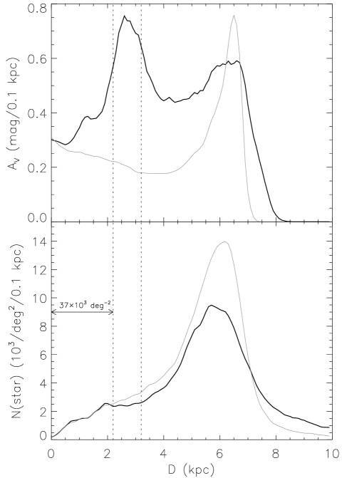
Figure 7: Extinction (top) and star density (bottom) along the Trifid line-of-sight. The black line is the average value for the region where $A_{V}>20$ mag in Fig. 6; the gray line is for the region where $A_{V}\in[0,1]$ mag. The dashed lines indicate the Trifid location at a distance of $2.7\pm 0.5$ kpc.

A three dimensional stellar model of the Galaxy (Robin et al., 2003) is used to simulate the stellar distribution along the line-of-sight towards the Trifid nebula. The simulated stars are not subjected to extinction and so they provide an estimate of the intrinsic color and distance of the stars along this line-of-sight. By comparing the color distribution of the unreddened, simulated, stars to the observed stellar color distribution it is possible to infer the extinction distribution along the line-of-sight (Marshall et al., 2006). We use observations from 2MASS, UKIDSS and GLIMPSE and use the Ks-[3.6] color to probe the line-of-sight extinction. This technique is relatively independent of the stellar counts and reflects the changing stellar color as a function of distance (see Marshall et al. 2006 for more details). Furthermore there is no need to remove foreground stars as we are comparing the observations to a model where all stars are included. However, care needs to be taken to ensure that the model is indeed representative of the observations, so the simulated catalog is cut at the completeness magnitude of the observations in the $K_{s}$, [3.6] and [4.5] bands. Recently, Marshall et al. (2009) improved on this method using a genetic algorithm to deduce the line-of-sight extinction necessary to reproduce the observed stellar color distribution along a given line-of-sight. This version is the one we chose to use as it provides higher angular resolution ($\sim$3 arcmin compared to 15 arcmin previously) and more sensitivity to extinction features within 2 kpc from the Sun. The resulting distances are subject to an uncertainty of roughly 15% but this may be higher at large distances and through high column densities. This results in a smearing out of extinction features along the line of sight, and could explain why, in Fig. 7, a narrow extinction peak is found at 6.5 kpc when the extinction is low but this same peak is found to be wider through the higher density lines-of-sight crossing the Trifid nebula. At such a distance the interstellar material can be related to several Galactic structures which are the molecular ring (about 3-4 kpc from the Galactic center), the start of the Norma Arm, and the extremity of the Galactic bar.

The results of the 3D modeling is presented in Fig. 7. The extinction profile for the region where $A_{V}>20$ mag (see Fig. 6) provides us with a direct estimation of the cloud distance. Fitting a Gaussian yields a distance of $2.7\pm 0.5$ kpc. The extension of the cloud along the line-of-sight is likely from 50 to 100 pc so the Gaussian standard deviation represents the uncertainty inherent to the 3D modeling, not the cloud size. The literature often refers to 1.7 kpc (Lynds et al., 1985) for the Trifid nebula distance although a serious alternative is proposed by Kohoutek et al. (1999) with a distance between 2.5 and 2.8 kpc. Both estimations are based on the photometry of the central stars. The second work is more complete as it uses more stars and includes spectroscopy and accurate photometry. Our analysis of the tridimensional stellar distribution unambiguously supports the long distance hypothesis which place the Trifid in the Scutum Arm (Vallée, 2008) rather than the Sagittarius Arm as generally reported. In the following we assume $d=2.7$ kpc.

For such a distance, the foreground star number is expected to be at least $37\times 10^{3}$ deg^-2 (see Fig. 7), or $11\times 10^{3}$ deg^-2 if we restrict the sample to 2MASS sources. This is in good agreement with the analysis presented in Sect. 2.2 where we found a total foreground star density of at least $37\times 10^{3}$ deg^-2 towards the dense region of the cloud and in agreement with the distribution of 8600 stars deg^-2 detected by 2MASS which was found to be uncorrelated with the extinction, i.e. foreground to the cloud. It worth noting the Sect. 2.2 results are also incompatible with the short distance hypothesis. The ¹²CO velocity obtained from Dame et al. (2001) shows a velocity structure consistent with our extinction distribution which corroborates our estimation. The Trifid molecular clouds LSR velocity is about 18-20 km s^-1. Assuming a Sun kinematic from McMillan & Binney (2010), a distance to the Galactic center of 7.8 kpc and a rotation speed of 247 km s^-1 the Trifid velocity corresponds to a kinematic distance of 3.2-3.4 kpc which is even larger than our estimation based on the stellar population model.

The 3D analysis estimates the diffuse extinction in this direction to $\sim$3 mag kpc^-1 and it shows that no other dense cloud significantly contaminates the Trifid line-of-sight. The stellar fraction at distance larger 8 kpc represents only 7.7% of the background stars at large extinction and 2.6% at small extinction. In both cases their median distance is $\sim$5.8 kpc. The zero point chosen for the extinction map (Fig. 6) is validated by the 3D study as 1) there is no peak at $\sim$3 kpc at low extinction and 2) it compensates for the diffuse extinction on the line-of-sight and the contamination at 6.5 kpc.

4.3 Cloud mass

The cloud mass is derived from the extinction map using the following relation (Dickman, 1978):

$$M=(\alpha d)^{2}\,\mu\,\frac{N_{H}}{A_{V}}\sum_{i}A_{V}(i)$$ (1)

where $\alpha$ is the angular size of a pixel map, $d$ the distance to the cloud, $\mu$ the mean molecular weight corrected for the helium abundance, and $i$ represents a pixel map. With the dust-to-gas ratio proposed by Savage & Mathis (1979), $N_{H}/A_{V}=1.87\times 10^{21}$ cm^-2 mag^-1 ($N_{H}=N_{HI}+N_{H_{2}}$) and a distance of 2.7 kpc, we obtain a mass of $5.8\times 10^{5}$ M_⊙. This value corresponds to twice the Orion (A+B) clouds mass (Cambrésy, 1999; Wilson et al., 2005). Figure 8 shows how the integrated mass distribution varies with the extinction within the cloud. Regions with visual extinction greater than 20 mag account for less than 4% of the total mass of the cloud. The index of the cumulative mass distribution, $\alpha$, changes at $A_{V}\approx 25$ mag by a factor of 2. For $M(A_{V})$ being the mass enclosed in the contour of extinction $A_{V}$, we have:

$$M(A_{V})=M(0)\times 10^{-\alpha A_{V}}$$ (5)

$$\mbox{ with }\left\{\begin{array}[]{l}\alpha=8.39\times 10^{-2}\mbox{ for }A_{V}\in[8,20]\\ \alpha=3.76\times 10^{-2}\mbox{ for }A_{V}\in[30,60]\end{array}\right.$$

Figure 8: Cumulative mass distribution for d=2.7 kpc. The $\alpha$ index is defined in Eq. 5.

The variation of $\alpha$ is not a side-effect of the map combination technique nor the application of a corrected extinction law at large $A_{V}$ since the variation is also observed for a raw extinction map obtained only from the [3.6]-[4.5] color-excess and assuming a constant extinction law. It is however difficult to interpret the index variation as a consequence of the dust transition responsible of the extinction law evolution. The two events occurring at the same level may just be a coincidence. The $N_{H}/A_{V}$ value is generally assumed to be universal although some authors suggested a decrease by a factor of 3 in deeply embedded regions (Winston et al., 2010). Dividing the mass estimate by any factor above a given extinction threshold would only produce an offset in Fig. 8, not a change of slope. A more complex evolution of $N_{H}/A_{V}$ with the extinction would affect differently the Fig. 8 distribution but it seems unlikely to only produce a sharp slope change.

Table 3: Properties of the more extended Trifid cores detected at millimeter wavelength (Lefloch et al., 2008). Masses are expressed assuming a distance of 2.7 kpc. The mass from dust continuum emission is derived using $T_{\rm dust}=15$ K and $\kappa_{1.25}=4.08\times 10^{-1}$ cm² gr^-1 (i.e. $C_{1.25}=7.336\times 10^{-27}$ cm² H^-1). By modifying these parameters the mass can be adjusted to the mass estimated from the dust extinction. The two last columns give these parameter values, providing only one of the two parameters is modified at the same time.

Name	Mass	Mass	$A_{V}$ (mag)			Surface	$\kappa$	$T_{\rm dust}$
$[$CLC98$]$	($M_{\odot}$)	($M_{\odot}$)	peak	median	outer	(arcmin2)	($\times$)	(K)
TC00	936	911	27	22.7	20.0	3.5	1.3	13
TC0	1607	1570	25	20.3	16.9	6.9	1.2	13
TC3	3535	2783	78	40.4	27.6	7.3	2.6	8
TC4	1149	945	52	32.8	23.7	3.0	2.7	8
TC5	3543	3087	53	25.5	18.1	11.6	1.7	11

The millimeter wavelength emission from the cold dust continuum has been mapped by Cernicharo et al. (1998) and Lefloch et al. (2008). They have detected several dust condensations from the 1.25 mm emission. For simplicity we designate these dust condensations TC NN as in the original papers. This is fine is the Trifid context but obviously ambiguous in the general context and the full SIMBAD name is actually [CLC98] TC NN. For the more extended condensations we compare the mass from the dust infrared extinction and 1.25 mm emission. The results are presented in Table 3. The mass from extinction is obtained by integrating the area defined in the map at 1.25 mm, convolved at 1 arcmin resolution, by the contour at $S_{1.25}=10$ mJy$/11^{\prime\prime}$ beam (red shaded area in Fig. 6). Because of the observational technique in the millimeter wavelengths, a spatial filtering removes the structure at scale larger than 4.5 arcmin in the dust continuum emission. To compare this map with the extinction map we scale it by adding the median extinction measured in the vicinity of each TC region. Basically the median extinction is measured in the area between the contours at $S_{1.25}=5$ and 10 mJy/11” around each condensation. The resulting offsets are given in the column labeled outer of Table 3. The mass from the map at 1.25 mm is derived assuming a dust temperature of 15 K and a dust opacity of $\kappa_{1.25}=4.08\times 10^{-1}$ cm² gr^-1 following the model B for $R_{V}=5.5$ by WD01. The corresponding extinction cross section per hydrogen atom is $C_{1.25}=7.336\times 10^{-27}$ cm² H^-1 after correction for the helium abundance and assuming a gas-to-dust ratio of 125 (Li & Draine, 2001). Lefloch et al. (2008) measured temperatures from 20 to 30 K using CO observations. The gas kinetic temperature and the dust temperature are however different in such regions and an arbitrary $T_{\rm dust}=15$ K is more appropriate. The masses we derived from the dust emission are systematically smaller. Two parameters, the temperature and the emissivity, can be adjusted to reach an agreement with the masses from extinction. While TC00 and T0 only need a small increase of the dust emissivity at 1.25 mm, or to decrease the temperature from 15 to 13 K, TC3/4/5 require a more significant emissivity increase by a factor 1.7 to 2.7. Using only the temperature as free parameter would lead to 11 to 8 K. Such low temperatures have already been reported by Désert et al. (2008) from submillimeter point sources observed by the Archeops experiment. However, the condensations we are dealing with cover an extended field from 3 to 12 arcmin². Assuming a minimum temperature of 12 K for TC3/4, an emissivity enhancement by a factor 1.9 would make the mass estimates in agreement. TC00 and TC0 are starless condensations while TC3/4/5 form stars and undergo shocks. Our analysis suggest the dust emissivity at millimeter wavelength is enhanced for these condensations, especially for the densest ones. Complementary observations at longer wavelengths, from Herschel and Planck, will permit to better understand the physical properties of the interstellar medium in the Trifid region. We plan to follow up this study as soon as the data from the Herschel Infrared Galactic Plane Survey (Hi-GAL, Molinari et al., 2010b) are available.

5 Conclusion

We performed a detailed analysis of the extinction in the molecular cloud associated with the Trifid nebula. The direction and the distance of this cloud is a major difficulty compared to the other similar investigations published in the literature. To overcome this specificity we proposed an original method which combines the color-excess mapping with the color-color diagram analysis. The gain in sensitivity with this method allowed us to measure to extinction law at 3.6, 4.5 and 5.8 $\mu$m and to unambiguously detect a variation at large absorption through an abrupt change of slope in the color-color plots. We interpreted this result as an evidence for a rapid dust evolution at high density like a new dust transition phase in the dense interstellar medium.

The extinction law parameters, $A_{\lambda}/A_{K_{s}}$, are found to be larger in the very dense cores of the cloud, in agreement with dust models. Our values for $A_{V}>20$ mag are however larger than predicted by WD01 for dense regions ($R_{V}=5.5$) and larger than previously reported in the literature at 3.6 $\mu$m. For $A_{V}<15$ mag, which does still refer to dense material, our values remarkably match those predicted by the model for $R_{V}=5.5$, as expected. Our study is not sensitive to the diffuse medium for which $R_{V}=3.1$ with a typical visual extinction as low as 1 mag. Moreover, Zasowski et al. (2009) found a correlation of the extinction law for the diffuse interstellar medium with the galactocentric radius. They concluded the extinction curve follows the dust model with $R_{V}=5.5$ for a galactocentric radius consistent with the Trifid distance. It suggests the so-called diffuse medium already contains big grains in this part of the Galaxy. If the diffuse medium at the Trifid distance behaves like the dense medium in the solar neighborhood we can imagine the Trifid dense cores are also affected by the distance with a flatter extinction law.

Using our varying extinction law we built a composite extinction map of the Trifid nebula region. The maximum visual extinction is 80 mag at 1 arcmin resolution. We have also investigated the matter distribution along the line-of-sight since several small clouds could have mimicked the presence of a single giant massive dark cloud. We found no significant contribution of other clouds in this direction and we were able to estimate the distance of the Trifid nebula at $2.7\pm 0.5$ kpc.

The Trifid molecular cloud is about twice the mass of the Orion molecular cloud. The comparison of the dust extinction and 1.25 mm continuum emission in the densest cores suggests the dust emissivity is probably enhanced by a factor of 2-3 in these regions. This cloud appears as a young and massive version of the Orion or Rosette regions. The Trifid represents an earlier evolutionary status in the star-formation process with a first generation of OB stars but no significant embedded cluster yet. Several protostars in TC3/4 are likely the precursors of such clusters. Longer wavelengths observations from Herschel and Planck are needed to better understand the dust properties and the interaction between the interstellar medium and the OB stars.