Implementation of Single-qubit and CNOT Gates by Anyonic Excitations of Two-body Topological Color Code

Abstract

The anyonic excitations of topological two-body color code model are used to implement a set of gates. Because of two-body interactions, the model can be simulated in optical lattices. The excitations have nontrivial mutual statistics, and are coupled to nontrivial gauge fields. The underlying lattice structure provides various opportunities for encoding the states of a logical qubit in anyonic states. The interactions make the transition between different anyonic states, so being logical operation in the computational bases of the encoded qubit. Two-qubit gates can be performed in a topological way using the braiding of anyons around each other.

I Introduction

A set of universal quantum gates is a set of basic gates in which any operation in a quantum computer can be decomposed. This means that any unitary operation can be expressed as a finite sequence of the gates from the set.nielsen ; miguel:rmp02 The gates are used to process and transform the encoded information on the quantum register. They are unitary operations acting on one or two qubits and transform their states. For instance the Hadamard gates and rotation about axes are among single-qubit gates, while the controlled-Phase gates is a two-qubit gate acting between control and target qubits. Any arbitrary unitary operation acting on array of qubits can be synthesized using above gates, i.e. they form a universal set.jean

The main challenge of quantum computation is to design ways in which the universal gates can be implemented avoiding the accumulation of errors during the processing. Any information processing task must be robust against decoherence, that is, as the gates are implemented, the stored information are not read out.

Topological models provide an opportunity to secure information from decoherence and perform implementation on encoded information fault-tolerantly as well.mochon ; freedman ; nayak:rmp08 A form to achieve fault-tolerance is by means of self-correcting quantum computers.hector:arxiv09 ; hamma:arxiv09 In the topological models, the quantum information is encoded on the global degrees of freedom. Since operating on the global degrees of freedom deserves non-local operations acting on large number of qubits, the local perturbations are not able to destroy the stored information. In fact the ground states of the topological model can be used as topological quantum memory.dennis The storing of quantum information is interesting, but one needs to process the stored information. To perform computation on the stored information, one may use the topological properties of the excitation appearing above the ground state. The excitations have exotic statistics that are neither fermion nor boson. They are anyons, instead. The non-trivial braiding of anyons can be used to construct gates. If under the monodromy operations on the excitation (winding of excitations around each other) the wavefunction of the system acquires a global phase, the respective anyons are called abelian anyons. But they could also be non-abelian in the sense that the evolution of the wave function is described by unitary matrices.

The famous Kitaev model on a honeycomb lattice have abelian and non-abelian anyonic states appearing at different regimes of couplings.kitaev1 In particular, the emerging abelian anyons can be used to perform single-qubit and two-qubit gates.Lloyd ; pachos Although such implementation by abelian anyons is interesting by itself, but creating a purely anyonic state with only low energy vortices in this model is challenging. This is important for physical applications. Anyonic excitations are created by applying local spin operators on the ground state of the Kitaev honeycomb model. But, any attempt to create anyons is spoiled by creation of high energy fermions.vidal1 ; vidal2

Topological color code model (TCC)hector1 ; hector2 presents another topological stabilizer model with enhanced computational capabilities such as transversal implementation of whole Clifford group. The code appears as ground state subspace of the two-body Hamiltonian defined on a rubby lattice.kargarian1 ; kargarian2 Emerging high energy fermions belong to different classes each of one color charge. In each class high energy excitations have fermionic statistics while fermions associated to different classes have mutual semionic statistics.hector3 This latter point implies that high-energy excitations are not only fermions but also anyons which is absent in the Kitaev model.

The aim of this paper is to use the anyonic character of the emerging high energy fermions in order to implement gates. Recently, experimental realizations of topological error correction codes have been implemented,expriment1 as well as experimental proposals for TCCs using Rydberg atoms expriment2 . We use various ways of encoding qubits. Once the qubit states are encoded into anyonic fermions, the proper implementation of single-qubit and two-qubit gates are instructed by manipulation of anyons. The fact that the quantum state of hard-core bosons (anyonic fermions) realized in optical lattices enlightens and motivates our construction for encoding and manipulation of information.exp_hardcore The creation and manipulation of anyonic fermions are done by interactions in the Hamiltonian which can be controlled in optical lattices. In particular, we will show that the manipulation of anyonic fermions can be used to implement the single-qubit $X$ and $Z$ gates in a non-topological way, and the two-qubit CNOT gate is topologically performed via the braiding of anyonic fermions.

The paper is organized as follows. In Sec.II we briefly review the two-body color code model and emerging anyonic fermions. In Sec.III we use these emerging excitations for encoding and implementation of single and two-qubit gates. The conclusions are presented in Sec.IV.

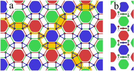
Figure 1: (color online) (a) A piece of rubby lattice. Links are colored according to the interaction between spins sitting at the vertices. Blue, red and green links stand for $\sigma^{z}\sigma^{z}$, $\sigma^{x}\sigma^{x}$ and $\sigma^{y}\sigma^{y}$, respectively. The plaquettes can also be colored accordingly, and the spins around a plaquette have the sam color with plaquette. A string-net is also shown, where three strings with different colors can meet at an effective site. (b) A pictorial representation of terms in Eq.4. From up to bottom: hopping, fusion, color switching and annihilation.

II emerging anyonic fermions

To see how high energy fermions appear, consider a set of spin-$1/2$ particles sitting at the vertices of the rubby lattice as shown in Fig.1. We assume the following interactions hold between spins.

$$H=-J_{x}\sum_{r-link}\sigma^{x}_{i}\sigma^{x}_{j}-J_{y}\sum_{g-link}\sigma^{y}_{i}\sigma^{y}_{j}-J_{z}\sum_{b-link}\sigma^{z}_{i}\sigma^{z}_{j},$$

where we are using three colors red, green and blue to distinguish between different links. Each colored link represents an interaction as in Eq.II. The plaquettes of the lattice are colored and vertices can also be colored accordingly. Associated with each colored plaquette, say blue hexagon in Fig.1, three local string operators can be realized.kargarian1 ; kargarian2 Such local operators, called plaquette operators, commute with each other and with the Hamiltonian in Eq.II. Hence, they are constants of motion and can be used to identify the local symmetry of the model. Let’s denote them by $P_{1}$, $P_{2}$ and $P_{3}$. The explicit expression of these operators are given in Appendix.B. By use of Pauli algebra, it’s immediate to check both of the following relations.

$$P_{1}^{2}=P_{2}^{2}=P_{3}^{2}=1,~{}~{}~{}P_{1}P_{2}P_{3}=-1.$$ (2)

These relations indicate that all three plaquette operators are not independent giving rise to the local gauge symmetry $\mathrm{Z_{2}}\times\mathrm{Z_{2}}$ of the color code model.

For any path on the lattice one can realize string operators in which the contribution of the vertices to the corresponding operator is determined by the outgoing link at each vertex. For example if a vertex on the string is crossed by a red link, its contribution to string operator is $\sigma^{x}$. A simple example of elementary string operators is shown in Appendix. B. Strings can be combined to form string-nets.kargarian1 ; kargarian2 A typical string-net is shown in Fig.1, where each colored string connects plaquettes with same color and three strings meet at a triangle. The number of integrals of motions is exponentially increasing. Let $3N_{s}$ be the total number of spins, so the number of plaquettes will be $N_{s}/2$. Regarding to the gauge symmetry of the model, the number of independent plaquette operators is $N_{s}$. This implies that there are $2N_{s}$ integrals of motion and allow us to divide the Hilbert space into $2^{N_{s}}$ sectors labeled by the eigenvalues of plaquette operators. However, the Hamiltonian Eq.II can not be exactly solved based on the integrals of motions. Moreover, because of four-valent structure of the lattice, unlike the Kitaev model the model is not exactly solvable in terms of mapping to Majorana fermions.kargarian1 ; feng:prl07 However, many features of the physics of the model can be treated by considering the limiting behavior of the model.

We divide the Hamiltonian in two parts as $H=H_{0}+V$, where the first term denotes the unperturbed Hamiltonian $H_{0}=-J_{z}\sum_{b-link}\sigma^{z}_{i}\sigma^{z}_{j}$ and the second term denotes the interaction between triangles as $V=-J_{x}\sum_{r-link}\sigma^{x}_{i}\sigma^{x}_{j}-J_{y}\sum_{g-link}\sigma^{y}_{i}\sigma^{y}_{j}$. In the isolated triangle limit, i.e. $J_{x}=J_{y}=0$, the lattice contains a collection of blue triangles. For each triangle the subspace spanned by polarized spins, up or down, has the minimum energy of $-3J_{z}$. Thus, the ground state of a triangle is two-fold degenerate and the excited states with energy of $J_{z}$ are six-fold degenerate. So the ground state of Hamiltonian is highly degenerated spanned by different configuration of polarized spins on triangles.

As the couplings $J_{x}$ and $J_{y}$ grow on, the ground state degeneracy is broken. The effects of perturbations can be teated by invoking the spin-boson transformation.kargarian1 ; hector3 The transformation is exact in which the spectrum of each triangle is replaced by an effective spin and an hard-core boson. Taking all possible degrees freedom of spins on a triangle into account, we find four possible cases for a boson to be on the triangle: nothing, red, green and blue. In fact the excitation of each triangle is revealed by a colored boson. The mapping from original degrees of freedoms to effective spin and hard-core bosons is given in Appendix.A. From now on triangles are addressed by effective sites forming a hexagonal lattice $\Lambda$. Thus, we distinguish between sites (triangles) and vertices. The letter $c$ is used for one of the colors, then a bar operation $\bar{c}$ transforms colors cyclically as $\bar{r}=g$, $\bar{g}=b$ and $\bar{b}=r$. We also use the notation convention $c|c:=x$,$\bar{c}|c:=y$ and $\bar{\bar{c}}|c:=z$.

We refer to a site by considering its position relative to a reference site: the notation $O_{,c}$ means $O$ applied at the site that is connected to a site of reference by a link with color $c$. The different terms in the Hamiltonian can then be interpreted in terms of effective spins and hard-core bosons as follows.kargarian1 ; hector3

$$H=-3N/4+Q-\sum_{\Lambda}\sum_{c\neq c^{\prime}}J_{c^{\prime}|c}T_{c}^{c^{\prime}},$$ (3)

with $N$ the number of sites ($N=N_{s}/3$), $Q:=\sum_{\Lambda}n$ the total number of hardcore bosons, the first sum running over the $N$ sites of the hexagonal lattice, the second sum running over the 6 combinations of different colors $c,c^{\prime}$ and

$$T_{c}^{c^{\prime}}=u_{c}^{c^{\prime}}+\frac{t_{c}^{c^{\prime}}+v_{c}^{c^{\prime}}}{2}+\frac{r_{c}^{c^{\prime}}}{4}+\mathrm{h.c.},$$ (4)

a sum of several terms for an implicit reference site, according to the notation convention defined above. The explicit expression of the terms appearing in the above equation is given in Appendix.A. They represent various bosonic processes including $t_{c}^{c^{\prime}}$: hopping bosons between sites, $v_{c}^{c^{\prime}}$: annihilation or creation of a pair of bosons, $u_{c}^{c^{\prime}}$: fusion of two bosons in two another one or splitting of one boson into two others and $r_{c}^{c^{\prime}}$: switching between colors of two bosons.hector3 A pictorial representation of these terms is shown in Fig.1b. We will use these processes as possible ways for encoding of qubit states.

By examining the hopping termswen it is simple to see that a colored hard-core boson is fermion, i.e. under the exchange of two hard-core bosons with same color a minus sign arises. This implies that in this model we are dealing with three classes of high-energy fermions each of one color. Although hard-core bosons in each class are fermions by themselves, they have mutual semionic statistics with respect to fermions in other classes. This means that if for example a blue high-energy fermion go around a green high-energy fermion, the wavefunction picks up a minus sign. This is the reason for the name of anyonic fermions.hector3

The appearance of such anyonic fermions is in sharp contrast with emerging high-energy fermions in the Kitaev model.vidal1 ; vidal2 In the latter model we are dealt with one class of high-energy fermions. This is rooted in the fact that in the Kitaev model there is only one type of strings carrying fermions, while in the color code model there are three different classes of strings forming string-net structure for the model. As long as the anyonic properties of excitations are important as in implementing one- and two-qubit gates, we can use colored high-energy fermions. This is the subject of the next section.

III encoding qubits and implementation of gates

As usual let $|0\rangle$ and $|1\rangle$ stand for the states of a qubit in the computational bases. These states first must be encoded in the states of the anyons, then manipulation of them is done by anyons. The contribution of the colors in the construction of the code makes it possible to use different methods for encoding. Once the encoding is done, a corresponding manipulation of anyons are assigned to implement gates.

III.1 Encoding in hopping process

The hopping of a $c$-fermion from a site to another one provides a natural way for encoding the states of a qubit. To this end, we encode the states of a qubit on a two-site model with an $c$-fermion. We define a local Hilbert space with two bases as $|c,0\rangle$ and $|0,c\rangle$ if first and second sites, respectively, are occupied by $c$-fermion. These states can be used to encode two states of a qubit. If $c$-fermion is on the first site, i.e. $|c,0\rangle$ , it corresponds to $|1\rangle$. Otherwise, it will encode the $|0\rangle$. A pictorial representation of such encoding has been shown in Fig.2a. Let $t_{c}$ operator stands for the hopping of $c$-fermion from one site to another one. Thus, the hopping operator just encodes the action of Pauli operator $\sigma^{x}$ in the space spanned by the states of qubit. In fact, the hopping process is just the NOT gate. The number operator $n_{c}$ at first site, which measures number of $c$-fermions at a site, can be used to simulate the $\sigma^{z}$ in the qubit space. In fact, the parity operator $p_{c}=1-2n_{c}$ gives a minus (plus) sign if the first site is occupied (unoccupied). With this realization of Pauli operators in terms of $c$-fermion process, we have all required ingredients for implementation of single-qubit $X$ and $Z$ gates. Notice that the latter gates are no longer performed in a topological way as we must switch between different states by means of local interactions, which are not protected.

How can we implement two-qubit gates? As we will see two-qubit gates require braiding of particles around each other. First we use two pairs of sites each encodes one qubit. Two qubits must be encoded by fermions with different colors in order for braiding to be nontrivial. To perform a two-qubit gate, one simply needs to take whatever is in the first site of the first qubit (control qubit), then move it around the first site of the second qubit (target qubit), as shown in Fig.2a. Trivially, if the first qubit is in the state $|0\rangle$, which corresponds to the situation in which the first site is empty, the braiding action leaves the second qubit unchanged. In other words, the second qubit is not braided any more. However, the nontrivial case will be achieved whenever both qubits are in the state $|1\rangle$. Only in this case the first sites of both qubits are occupied by the fermions with different colors, namely first site of control qubit is occupied with a $c$-fermion and first site of the target qubit is occupied with a $\bar{c}$-fermion. Thus, the braiding of $c$-fermion around the $\bar{c}$-fermion gives rise to overall factor (here minus) for the states of two qubits.

All possible cases of braiding can be summarized as follows:

$$|0,r\rangle|0,g\rangle\rightarrow|0,r\rangle|0,g\rangle~{}~{}\Leftrightarrow~{}~{}|00\rangle\rightarrow|00\rangle,$$

$$|0,r\rangle|g,0\rangle\rightarrow|0,r\rangle|g,0\rangle~{}~{}\Leftrightarrow~{}~{}|01\rangle\rightarrow|01\rangle,$$

$$|r,0\rangle|0,g\rangle\rightarrow|r,0\rangle|0,g\rangle~{}~{}\Leftrightarrow~{}~{}|10\rangle\rightarrow|10\rangle,$$

$$|r,0\rangle|g,0\rangle\rightarrow-|r,0\rangle|g,0\rangle\Leftrightarrow~{}|11\rangle\rightarrow-|11\rangle.$$ (5)

But the above evolution of states of two qubits under braiding is just the controlled phase gate, which can be turned into the CNOT-gate by applying the $\sigma^{x}$ to the target qubit. The braiding process can be applied between any two arbitrary qubits. We should only note that two qubits are encoded by fermions with different colors, since fermions with different colors have semionic mutual statistics. The braiding evolution is resilient to any deformation of the braiding path so long as only the first site of the target qubit is braided. The ability to perform two-qubit gate together with one-qubit $X$ and $Z$ gates make the implementation of part of a universal set of gates for quantum computation. For full implementation of universal gates, we should be able to implement two other single qubit gates, the Hadamard and phase gates, as well, which it seems that would not be possible in this setting.

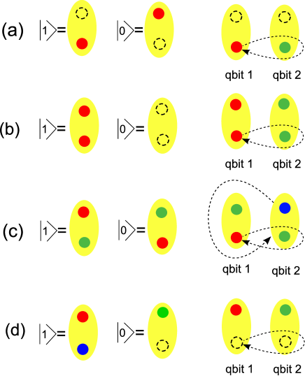
Figure 2: (color online) Different processes that make the encoding of a logical qubit (left) and the corresponding braiding process for implementation of two-qubit gate (right). Each ellipse shows a two-site model, and arrow dashed line indicates the braiding path. The processes are (a) the hopping process (b) the annihilation process (c) the color switching process and (d) the fusion process.

III.2 Encoding by annihilation/creation process

Again a two-site model is used to encode a single qubit. An annihilation/creation process will annihilate/create a pair of $c$-fermions on two sites. Let operator $v_{c}$ stands for annihilation of pair of $c$-fermions on two sites. Given the empty or filled sites, the states of a qubit can be simply encoded. The empty sites, i.e. $|0,0\rangle$, and filled sites, i.e. $|c,c\rangle$, are properly adjusted to encode the states $|0\rangle$ and $|1\rangle$ of qubit, respectively. A schematic representation of this encoding is shown in Fig.2b. The annihilation and creation operators switch between two different states of two-site model, which in the logical space is interpreted as Pauli operator $\sigma^{x}$. The parity of either first or second sites can be used to encode the $\sigma^{z}$ Pauli operator in the logical space. Therefore, the annihilation/creation and parity operators allows one to perform single-qubit $X$ and $Z$ gates in the logical space of a qubit.

Implementation of two-qubit gate is done by braiding of $c$-fermions. Two qubits are encoded in two pairs of sites separately. But the corresponding logical space of each qubit carries a distinct color. For example, as shown in Fig.2b, we assume the logical space of first qubit (control) has red fermion while the second qubit (target) has green fermion. Choosing fermions with different colors is important for using the benefit of nontrivial braiding between them. We suppose a process through which the contents of the first site of control qubit move around the first site of target qubit. Definitely, the logical states $|00\rangle$ and $|01\rangle$ remains unchanged through braiding since the first site of target qubit is not braided at all. The logical state $|10\rangle$ also doesn’t change since the $c$-fermion moves around an empty site. However, when the $\bar{c}$-fermion of target qubit is braided by the $c$-fermion of control qubit, a global phase (here minus sign) arises. This latter case corresponds to the evolution of logical state $|11\rangle$ into $-|11\rangle$ that is just the controlled-phase gate.

Regarding to Fig.2b, the resulted two-qubit gate is as follows

$$|0,0\rangle|0,0\rangle\rightarrow|0,0\rangle|0,0\rangle~{}~{}\Leftrightarrow~{}~{}|00\rangle\rightarrow|00\rangle,$$

$$|0,0\rangle|g,g\rangle\rightarrow|0,0\rangle|g,g\rangle~{}~{}\Leftrightarrow~{}~{}|01\rangle\rightarrow|01\rangle,$$

$$|r,r\rangle|0,0\rangle\rightarrow|r,r\rangle|0,0\rangle~{}~{}\Leftrightarrow~{}~{}|10\rangle\rightarrow|10\rangle,$$

$$|r,r\rangle|g,g\rangle\rightarrow-|r,r\rangle|g,g\rangle\Leftrightarrow~{}|11\rangle\rightarrow-|11\rangle.$$ (6)

Therefore, the encoding of logical states into annihilation/creation process and braiding evolution provide an alternative way for constructing a set of gates.

III.3 Encoding in color switching process

Two colored fermions with different colors can interchange their colors by tuning interaction between spins as in Hamiltonian of Eq.II. To have a concrete discussion consider two sites carrying fermions each of one color. A pictorial representation is shown in Fig.2c, where we used red and green colors for fermions. Let $|r,g\rangle$ be a state of fermions in which first and second sites carry red and green fermions, respectively. An color switching operator $r_{c}=r_{c,1}r_{c,2}$, where $r_{c,1}$ and $r_{c,2}$ act on first and second sites, respectively, takes the state $|\bar{c},\bar{\bar{c}}\rangle$ and transforms it as $r_{c}|\bar{c},\bar{\bar{c}}\rangle=|\bar{\bar{c}},\bar{c}\rangle$. Thus for each color $c$ two states $|\bar{c},\bar{\bar{c}}\rangle$ and $|\bar{\bar{c}},\bar{c}\rangle$ are used to encode the computational states of a logical qubit. The respective qubit is referred as $c$-qubit. When a switching operator turns on, one may take it into account as the operation of $\sigma^{x}$ in the computational bases. Thus the transition from $|0\rangle$ into $|1\rangle$ can be performed by means of color switching. A phase shift of a qubit is operated by parity measurement of the first site. Defining $p_{\bar{\bar{c}}}=1-2n_{\bar{\bar{c}}}$, it leaves $|\bar{c},\bar{\bar{c}}\rangle$ unchanged, but gives a minus sign upon the measurement of $|\bar{\bar{c}},\bar{c}\rangle$ as $p_{\bar{\bar{c}}}|\bar{\bar{c}},\bar{c}\rangle=-|\bar{\bar{c}},\bar{c}\rangle$. It results in rising phase difference between $|0\rangle$ and $|1\rangle$ states.

As before, the realization of two-qubit gates is based on the braiding of $c$-fermions sitting at sites. A two-qubit gate must be implemented between two qubits with different colors. Namely, we should consider $c-$ and $\bar{c}-$qubits. For instance, one may consider the situation depicted in Fig.2c, where we are dealing with a $b$-qubit as qbit1 and $r$-qubit as qbit2. The states of either qubit are encoded according to their colors as above. In particular, as shown in Fig.2c, the states of the encoded control qubit are $|r,g\rangle$ and $|g,r\rangle$, and the corresponding states of the target qubit are $|g,b\rangle$ and $|b,g\rangle$. Now we can offer an instruction for the braiding of fermions that permits the implementation of two-qubit gate. The instruction includes two sequential braiding processes: (i) the first site of control qubit moves around the first site of target qubit, then (ii) the target qubit entirely moves around the control qubit or vice versa. If the order of two processes are reversed, the final result of braiding remains unchanged. Such processes are shown in Fig.2c.

It is simple to check the effect of above evolution on all possible states of two qubits. The results are as follows.

$$|r,g\rangle|g,b\rangle\rightarrow|r,g\rangle|g,b\rangle~{}~{}\Leftrightarrow~{}~{}|00\rangle\rightarrow|00\rangle,$$

$$|r,g\rangle|b,g\rangle\rightarrow|r,g\rangle|b,g\rangle~{}~{}\Leftrightarrow~{}~{}|01\rangle\rightarrow|01\rangle,$$

$$|g,r\rangle|g,b\rangle\rightarrow-|g,r\rangle|g,b\rangle\Leftrightarrow~{}|10\rangle\rightarrow-|10\rangle,$$

$$|g,r\rangle|b,g\rangle\rightarrow|g,r\rangle|b,g\rangle~{}~{}\Leftrightarrow~{}~{}|11\rangle\rightarrow|11\rangle,$$ (7)

which clearly manifest the braiding process encodes the controlled-phase gate in the logical space of two qubits. It is not the only way of performing two-qubit gate. One may consider another scenario for braiding. First take the first site of control qubit and move it around the fist site of target qubit, then the first (second) site of either control or target qubit is braided by second (first) site. They eventually give rise to the above results of performing two-qubit gate in the logical space. Being able to perform the braiding of fermions around each other by either above methods, we see that the color switching between fermions together with the braiding provide what we need to perform the single qubit $X$ and $Z$ gates and two-qubit gate.

III.4 Encoding in fusion process

A significant feature of the two-body color code mode is the existence of 3-vertex interaction in the interacting fermionic processes.hector3 The existence of 3-vertex interaction exhibits in the representation in terms of effective sites, three colored fermions can fuse into vacuum making the high-energy fermions highly interacting. In other words two high-energy fermions with different colors can fuse to the third one. This is called a fusion process. Let $u_{c}$ denotes the fusion operator that fuses a $c$-fermion and $\bar{c}$($\bar{\bar{c}}$)-fermion into a $\bar{\bar{c}}$($\bar{c}$)-fermion.

One may wonder if fusion process could be used to encodes the states of a logical qubit. Again consider a two-site model. Suppose first and second sites are occupied by blue and green fermions, respectively, as shown in Fig.2d. The result of fusion process is that the first site is unoccupied and the the second site is occupied by a red fermion. Indeed, through the fusion process the fermion on the first site is annihilated and the color of fermion on the second site is switched. Let $|c,\bar{c}\rangle$ and $|0,\bar{\bar{c}}\rangle$ stand for states of two-site model through a fusion process. We exploit these two states to encode the computational bases of a qubit. We call such a qubit as a $\bar{\bar{c}}$-qubit. By definition, the state $|0,\bar{\bar{c}}\rangle$ is used to encode $|0\rangle$ and the state $|c,\bar{c}\rangle$ encodes $|1\rangle$. An imaginative picture of this encoding is shown in Fig.2d. The fusion operator and its conjugate (splitting) transform the states into each other, which eventually can be used to encode the $\sigma^{x}$ Pauli operator in logical space. The parity operator can be adapted in which encodes the $\sigma^{z}$. In fact the parity of fist site leaves the $|0,\bar{\bar{c}}\rangle$ unchanged while shifts the phase for the state $|c,\bar{c}\rangle$. Thus, the fusion process has all necessary ingredients for implementation of $X$ and $Z$ gates.

As before performing two-qubit operation requires braiding of fermions around each other. To have a nontrivial braiding process, we need to encode two qubits in different sets of states characterized by different colors. To have a concrete discussion, let consider the case shown in Fig.2d, where two qubits (qbit1 and qbit2) are red and green ones. The red qubit serves as control qubit and the green qubit serves as target one. With the above definition for the states of the sites, the states that encode the red qubit (qbit1) are as $|0,r\rangle$ and $|g,b\rangle$, and the states that encode the green qubit (qbit2) are as $|0,g\rangle$ and $|b,r\rangle$. The braiding scheme is simple: the first site of the target qubit must be braided by the entire contents of the first site of the control qubit, as shown in Fig.2d. If the control qubit is the state $|0\rangle$, its first site carries no fermion resulting in a trivial braiding. The same holds when the target qubit is in the state $|0\rangle$. By inspection we see that the only nontrivial case happens when both qubits are in the $|1\rangle$ state. The effect of braiding on all possible states of two qubits are as follows.

$$|0,r\rangle|0,g\rangle\rightarrow|0,r\rangle|0,g\rangle~{}~{}\Leftrightarrow~{}~{}|00\rangle\rightarrow|00\rangle,$$

$$|0,r\rangle|b,r\rangle\rightarrow|0,r\rangle|b,r\rangle~{}~{}\Leftrightarrow~{}~{}|01\rangle\rightarrow|01\rangle,$$

$$|g,b\rangle|0,g\rangle\rightarrow|g,b\rangle|0,g\rangle~{}~{}\Leftrightarrow~{}~{}|10\rangle\rightarrow|10\rangle,$$

$$|g,b\rangle|b,r\rangle\rightarrow-|g,b\rangle|b,r\rangle\Leftrightarrow~{}|11\rangle\rightarrow-|11\rangle.$$ (8)

Thus, we see that the fusion process encodes the a single qubit and if supplemented with braiding as stated above, the implementation of $X$ and $Z$ gates and CNOT becomes possible.

IV summary and concluding remarks

In this work the problem of implementation of a set of gates, which includes single-qubit (X and Z) and two-qubit (CNOT) gates, using the anyonic excitations of the two-body color code model was studied. Because of its underlying lattice structure, we can realize three types of strings each of one color that can form a string-net structure. The excitation spectrum of the model can be realized by the existence of three families of high-energy excitations. Each family is characterized by a color charge. The particle-like excitation in each family are fermions by themselves, but excitations from different families have a semionic mutual statistics, i.e. they are the anyonic fermions. This latter point is in sharp contrast with Kitaev honeycomb model, where the high-energy excitations have only fermionic statistics since they emerge from only one type of string. Therefore, it seems that the anyonic properties of high-energy fermions in the color code can be used for implementation of gates in quantum information tasks.

The fermions in the color code model undergo several processes such as hopping from site to another, annihilation/creation of pair of fermions on two sites, switching colors between fermions on two sites and fusion of fermions. All of them are driven by the terms in the Hamiltonian. Each process can be adjusted in such a way that encodes the states of a logical qubit. Namely, the computational bases are encoded in a two-site model including colored fermions, and the respective operation of fermionic process is translated into the Pauli operators. Thus, the $X$ and $Z$ single-qubit gates can be implemented by fermionic process. Neither encoding qubits nor implementation of latter single-qubit gates are topologically protected, thus they may suffer from the local perturbations. However, a successful implementation depends on ability of controlling fermionic quasiparticles.

Implementation of two-qubit gates require braiding of fermions. The states of control and target qubits must be encoded in separate pairs of sites. One may build those pairs in which they carry fermions with different color charges. In that case since they belong to different families of fermions, the braiding process can give rise to a nontrivial phase being suitable for performing of a two-qubit gate, the CNOT gate. Once a qubit is encoded in a fermionic process, the corresponding braiding encodes the controlled-phase gate. The implementation is topological as the path of braiding does not matter so long as an colored fermion is braided by another one.

Although performing the single-qubit gates are not topological, it is done in a way that is different from the manipulation of anyons in the Kitaev model. In the latter model implementation of single-qubit gates is done in a dynamical way, which needs rotation of spins to alter the anyonic state leading to switching between computational bases. But in the color code model the manipulation of colored fermions via any processes is driven by interaction terms in the Hamiltonian. Therefore, one only needs to control the interacting terms in which the proper manipulation occurs. Another advantage of our construction is that a quantum state of hard-core boson can be simulated in optical lattices.exp_hardcore

One may think that the process of braiding could accumulate errors in the system. But by a method based on the trapping potential,pachos the particle can move around immune. Therefore, the fermionic processes in the color code model encode the logical qubit and due to the nontrivial braiding of fermions with different color charge, the implementation of some gates becomes possible. An arbitrary quantum information task includes preparation of an initial state, implementation set of universal gates and measurements. The initial state can be prepared by an array of two-site models and filling the sites with colored fermion. The implementation of single-qubit gates ($X$ and $Z$) are performed by fermionic process introduced in preceding section and the two-qubit gates are done through the proper braiding of fermions around each other. Finally, the resulted state can be measured by determining how sites have been occupied by fermions.

Appendix A Bosonic mapping

The mapping between the original spin degrees of freedom on a triangle and effective spin coupled to a hard-core boson is as follows.kargarian1 ; hector3

$$|\!\Uparrow,0\rangle\equiv|\!\uparrow\uparrow\uparrow\rangle,~{}~{}~{}~{}~{} |\!\Downarrow,0\rangle\equiv|\!\downarrow\downarrow\downarrow\rangle$$

$$|\!\Uparrow,\mathrm{r}\rangle\equiv|\!\uparrow\downarrow\downarrow\rangle,~{}~{}~{}~{}~{} |\!\Downarrow,\mathrm{r}\rangle\equiv|\!\downarrow\uparrow\uparrow\rangle$$

$$|\!\Uparrow,\mathrm{g}\rangle\equiv|\!\downarrow\uparrow\downarrow\rangle,~{}~{}~{}~{}~{} |\!\Downarrow,\mathrm{g}\rangle\equiv|\!\uparrow\downarrow\uparrow\rangle$$

$$|\!\Uparrow,\mathrm{b}\rangle\equiv|\!\downarrow\downarrow\uparrow\rangle,~{}~{}~{}~{}~{} |\!\Downarrow,\mathrm{b}\rangle\equiv|\!\uparrow\uparrow\downarrow\rangle,$$ (9)

where the $\Uparrow$($\Downarrow$) and $\uparrow$($\downarrow$) stand for the states of effective spin sitting at a site and original spin sitting at a vertex of rubby lattice, respectively.

At each site we can introduce the color annihilation operator as $b_{c}:=|0\rangle\langle c|$. The number operator $n$ and color number operator $n_{c}$ are

$$n:=\sum_{c}n_{c},\qquad n_{c}:=b^{\dagger}_{c}b_{c}.$$ (10)

In terms of operators, the mapping Eq.9 can be expressed as follows.

$$\sigma^{z}_{c}\equiv\tau^{z}\otimes p_{c},\quad\sigma^{\nu}_{c}\equiv\tau^{\nu}\otimes(b_{c}^{\dagger}+b_{c}+s_{\nu}r_{c}),$$ (11)

where $\nu=x,y$, $s_{x}:=-s_{y}:=1$, the symbols $\tau$ denote the Pauli operators on the effective spin and we are using the color parity $p_{c}$ and the $r_{c}$ operators defined as

$$p_{c}:=1-2(n_{\bar{c}}+n_{\bar{\bar{c}}}),\qquad r_{c}:=b^{\dagger}_{\bar{c}}b_{\bar{\bar{c}}}+b^{\dagger}_{\bar{\bar{c}}}b_{\bar{c}}.$$ (12)

The explicit expressions of terms appearing in Eq.4 are

$$t_{c}^{c^{\prime}}:=\tau_{c}^{c^{\prime}}b_{c}b^{\dagger}_{c,c^{\prime}},~{}~{}r_{c}^{c^{\prime}}:=\tau_{c}^{c^{\prime}}r_{c}r_{c,c^{\prime}},$$

$$u_{c}^{c^{\prime}}:=s_{c^{\prime}|c}\tau_{c}^{c^{\prime}}b_{c}r_{c,c^{\prime}},~{}~{}v_{c}^{c^{\prime}}:=\tau_{c}^{c^{\prime}}b_{c}b_{c,c^{\prime}},$$ (13)

where we are using the notation

$$\tau_{c}^{c^{\prime}}:=\tau^{c^{\prime}|c}\tau_{,c^{\prime}}^{c^{\prime}|c}.$$ (14)

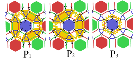
Figure 3: (color online) A representation of an elementary plaquette. With each plaquette we attach three local operators shown by yellow (light) string. The explicit expression of these operators is given by product of Pauli matrices acting on vertices labeled by $x$, $y$ and $z$ standing for $\sigma^{x}$, $\sigma^{y}$ and $\sigma^{z}$, respectively.

Appendix B Plaquette operators

On the rubby lattice a plaquette is defined by an inner hexagon with six triangles surrounding it. So each plaquette has eighteen vertices as shown in Fig.3. With each plaquette we attached three plaquette operators $P_{1}$, $P_{2}$ and $P_{3}$ having following properties.

$$[P_{i},P_{j}]=0~{}~{}\mathrm{and}~{}~{}[P_{i},H]=0~{}~{}\forall i,j.$$ (15)

The explicit expressions are as follows.

$$P_{1}=\prod_{l}\sigma^{\nu_{l}}_{l},~{}P_{2}=\prod_{k}\sigma^{\nu_{k}}_{k},~{}P_{3}=\prod_{m}\sigma_{m}^{z},$$ (16)

where products in $P_{1}$ and $P_{2}$ go over eighteen vertices with Pauli matrices $\sigma^{x}$ and $\sigma^{y}$, and product in $P_{3}$ goes over six vertices with all $\sigma^{z}$ as shown in Fig.3. $\nu_{l}$ and $\nu_{k}$ stand for $x$ or $y$ as shown besides vertices. Note that such identifications for local strings can be used to color the plaquettes and vertices of the lattice. We define the $P_{1}$ string as red string in which its fat parts (stretched yellow hexagon) connect red plaquettes, and we use green color for $P_{2}$. The third string is defined as a blue string surrounding around the internal hexagon. With this convention other plaquettes of lattice are colored accordingly. Having colored hexagons, we can simply color vertices: they have same color with the inner hexagon.

References

References

- (1) M. Nielsen and I. Chuang, Quantum Computation and Quantum Information, Cambridge University Press, 2000.
- (2) A. Galindo and M. A. Martin-Delgado, Rev. Mod. Phys. 74, 347 (2002).
- (3) Jean-Luc Brylinski, Ranee Brylinski, Mathematics of Quantum Computation, Chapman-Hall/CRC Press, 2002. quant-ph/0108062.
- (4) C. Mochon, Phys. Rev. A 67, 022315 (2003).
- (5) M. Freedman, M. Larsen, and Z. Wang, Comm. Math. Phys. 227, 605(2002).
- (6) Chetan Nayak, Steven H. Simon, Ady Stern, Michael Freedman and Sankar Das Sarma, Rev. Mod. Phys. 80, 1083 (2008).
- (7) Hector Bombin, Ravindra W. Chhajlany, Michal Horodecki, and Miguel-Angel Martin-Delgado, arXiv:0907.5228.
- (8) Alioscia Hamma, Claudio Castelnovo, Claudio Chamon, Phys. Rev. B 79, 245122 (2009)
- (9) E. Dennis, A. Kitaev, A. Landahl, and J. Preskill, J. Math. Phys. (N.Y.) 43, 4452 (2002).
- (10) A.Yu. Kitaev, Ann. Phys. (N.Y.) 303, 2 (2003); ibid 2, 321 (2006).
- (11) S. Lloyd, Quant. Inf. Proc. 1, 13 (2002).
- (12) J. K. Pachos, Int. J. Quant. Info, 4, No.6 (2006) 947.
- (13) K.P. Schmidt, S. Dusuel, J. Vidal, Phys. Rev. Lett. 100, 177204 (2008).
- (14) J. Vidal, K.P. Schmidt, S. Dusuel, Phys. Rev. B 78, 245121 (2008).
- (15) H. Bombin and M. A. Martin-Delgado, Phys. Rev. Lett. 97, 180501 (2006).
- (16) H. Bombin and M. A. Martin-Delgado, Phys. Rev. A. 76, 012305 (2007).
- (17) M. Kargarian, H. Bombin and M. A. Martin-Delgado, New J. Phys. 12, 025018 (2010).
- (18) H. Bombin, M. Kargarian and M. A. Martin-Delgado, Fortsch. Phys. 57, 1103 (2010).
- (19) H. Bombin, M. Kargarian and M. A. Martin-Delgado, Phys. Rev. B 80, 075111 (2009).
- (20) Xing-Can Yao, Tian-Xiong Wang, Hao-Ze Chen, Wei-Bo Gao, Austin G. Fowler, Robert Raussendorf, Zeng-Bing Chen, Nai-Le Liu, Chao-Yang Lu, You-Jin Deng, Yu-Ao Chen, Jian-Wei Pan, Nature 482, 489-494 (2012).
- (21) Hendrik Weimer, Markus Müller, Igor Lesanovsky, Peter Zoller, Hans Peter Büchler, Nature Phys. 6, 382 (2010).
- (22) B. Capogrosso-Sansone, C. Trefzger, M. Lewenstein, P. Zoller, G. Pupillo, Phys. Rev. Lett. 104, 125301 (2010).
- (23) X.-Y. Feng, G.-M. Zhang, T. Xiang, Phys. Rev. Lett. 98, 087204 (2007).
- (24) M. Levin, X.-G. Wen, Phys. Rev. B 67, 245316 (2003).