The optimal aspect ratio for piecewise quadratic
anisotropic finite element approximation

Abstract

Mesh adaptation for finite element approximation is a procedure used in numerous applications. The use of thin and long anisotropic triangles improves the efficiency of the procedure.

When piecewise linear finite elements are used, the aspect ratio for mesh adaptation is generally dictated by the absolute value of the (estimated) hessian matrix of the approximated function. We give in this paper the corresponding aspect ratio for piecewise quadratic finite elements.

Keywords—  Anisotropic finite elements, Adaptive meshes, Interpolation, Nonlinear approximation.

1 Introduction

Consider a bounded polygonal domain $\Omega\subset{\rm\hbox{I\kern-1.99997pt\hbox{R}}}^{2}$, a sufficiently smooth function $f:\Omega\to{\rm\hbox{I\kern-1.99997pt\hbox{R}}}$, and an integer $m\geq 2$. We introduce the problem of optimal mesh adaptation

$$\min\{\#({\cal T});\,{\cal T}\text{ s.t. }\|\nabla(f-\operatorname{{\rm I}}_{\cal T}^{m-1}f)\|_{L^{2}(\Omega)}\leq\varepsilon\},$$ (1)

where ${\cal T}$ stands for an arbitrary triangulation of $\Omega$, and $\#({\cal T})$ for its cardinality. Here $\operatorname{{\rm I}}_{\cal T}^{m-1}$ denotes the Lagrange interpolation operator onto finite elements of degree $m-1$ on ${\cal T}$.

In practical applications, the problem (1) is generally intractable for at least three reasons. 1: The function $f$ may have complicated local features, difficult to analyze. We thus first make a local analysis based on Taylor developments. 2: The collection of triangular meshes of $\Omega$ is a combinatorial set and problems such as (1) are typically NP-complete (after discretization). We avoid this problem by first considering the case of a single triangle. 3: Currently available anisotropic mesh generation algorithms only give control on the aspect ratio and orientation of the generated triangles, but not on their other features. We thus only optimize this aspect ratio.

2 An optimization problem

We denote by ${\rm\hbox{I\kern-1.99997pt\hbox{P}}}_{m-1}$ the space of bivariate polynomials of degree $\leq m-1$, and by ${\rm\hbox{I\kern-1.99997pt\hbox{H}}}_{m}$ the space of homogeneous polynomials of degree $m$. If $f\in C^{m}(\Omega)$, if $z\in\Omega$ is fixed and if $h\in{\rm\hbox{I\kern-1.99997pt\hbox{R}}}^{2}$ is small, then locally

$$f(z+h)=\mu_{z}(h)+\pi_{z}(h)+o(|h|^{m}),$$ (2)

for some $\mu_{z}\in{\rm\hbox{I\kern-1.99997pt\hbox{P}}}_{m-1}$ and $\pi_{z}\in{\rm\hbox{I\kern-1.99997pt\hbox{H}}}_{m}$. If $T$ is a sufficiently small triangle, we thus have at least heuristically on $T$

$$\nabla(f-\operatorname{{\rm I}}_{T}^{m-1}f)\simeq\nabla(\pi_{z}-\operatorname{{\rm I}}_{T}^{m-1}\pi_{z}),$$ (3)

since the Lagrange interpolation operator $\operatorname{{\rm I}}_{T}^{m-1}$ on the triangle $T$ reproduces the elements of ${\rm\hbox{I\kern-1.99997pt\hbox{P}}}_{m-1}$.

For any triangle $T$ and any $f\in H^{1}(T)\cap C^{0}(T)$, we define the averaged $H^{1}$ interpolation error $e_{T}(f)_{m}$ as follows

$$e_{T}(f)_{m}^{2}:=\frac{1}{|T|}\int_{T}|\nabla(f-\operatorname{{\rm I}}_{T}^{m-1}f)|^{2}.$$

The local counterpart of (1) is the problem of the optimal triangle : find for all $\pi\in{\rm\hbox{I\kern-1.99997pt\hbox{H}}}_{m}$

$$\sup\{|T|;\,T\text{ s.t. }e_{T}(\pi)_{m}\leq 1\}.$$ (4)

Indeed the cardinality of a triangulation is inversely proportional to the area of its elements. This approach is developed in Chapter 2 of [1] and leads to asymptotically optimal error estimates of (1) as $\varepsilon\to 0$ (or more precisely estimates of $\varepsilon$ as $\#({\cal T})\to\infty$, which is equivalent). Unfortunately these estimates are not completely realistic for applications because currently available numerical anisotropic mesh generators only control the aspect ratio and orientation of the generated triangles.

For each triangle $T$, of vertices $v_{1}$, $v_{2}$ and $v_{3}$, we denote by $z_{T}:=(v_{1}+v_{2}+v_{3})/3$ its barycenter. We denote by $S_{2}^{+}$ the collection of $2\times 2$ symmetric positive definite matrices, and we define a matrix ${\cal H}_{T}\in S_{2}^{+}$ by the equality

$${\cal H}_{T}^{-1}:=\frac{2}{3}\sum_{1\leq i\leq 3}(v_{i}-z_{T})(v_{i}-z_{T})^{\mathrm{T}}.$$

If $A$ is an invertible $2\times 2$ matrix and if $T^{\prime}$ is mapped onto $T$ by the linear map $z\mapsto Az$, then one easily checks that

$${\cal H}_{T^{\prime}}=A^{\mathrm{T}}{\cal H}_{T}A.$$ (5)

By construction the triangle ${T_{\rm eq}}$ of vertices $(\cos(2k{\text{\large$\boldsymbol{\pi}$}}/3),\sin(2k{\text{\large$\boldsymbol{\pi}$}}/3))_{0\leq k\leq 2}$ satisfies ${\cal H}_{T_{\rm eq}}=\operatorname{Id}$. Combining these two properties, Proposition 5.1.3 in [1] establishes that for any triangle $T$

$$|T|\sqrt{\det{\cal H}_{T}}=|{T_{\rm eq}}|,$$

and that there exists a rotation $U$ (depending on $T$) such that

$$z\mapsto U{\cal H}_{T}^{\frac{1}{2}}(z-z_{T})$$ (6)

maps $T$ onto ${T_{\rm eq}}$ (the power $\alpha$ of a symmetric positive definite matrix is obtained by elevating the eigenvalues to the power $\alpha$ in a diagonalization). Furthermore the ellipse of minimal volume containing $T$ is $\mathcal{E}_{T}:=\{z;\,(z-z_{T})^{\mathrm{T}}{\cal H}_{T}(z-z_{T})\}$, see Fig 1. The matrix ${\cal H}_{T}$ thus encodes the area, the aspect ratio and the orientation of $T$.

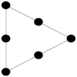
Fig. 1: Lagrange interpolation points for ${\rm\hbox{I\kern-1.99997pt\hbox{P}}}_{1}$ and ${\rm\hbox{I\kern-1.99997pt\hbox{P}}}_{2}$ finite elements (left), triangle $T$ and associated ellipse $\mathcal{E}_{T}$ (right).

For each $M\in S_{2}^{+}$ and each $\pi\in{\rm\hbox{I\kern-1.99997pt\hbox{H}}}_{m}$ we define

$$e_{M}(\pi)_{m}:=\sup\{e_{T}(\pi)_{m};\,T\text{ s.t. }{\cal H}_{T}=M\}.$$

We finally introduce for each $\pi\in{\rm\hbox{I\kern-1.99997pt\hbox{H}}}_{m}$ the problem of the optimal aspect ratio for ${\rm\hbox{I\kern-1.99997pt\hbox{P}}}_{m-1}$ interpolation

$$\inf\{\det M;\,M\in S_{2}^{+}\text{ s.t. }e_{M}(\pi)_{m}\leq 1\}.$$ (7)

3 Main result

Our main result is the solution of the optimization problem (7) in the case of piecewise linear and piecewise quadratic finite elements. The piecewise quadratic case is entirely new and gives a well founded answer to a long standing question: which aspect ratio, depending on the third derivatives of the approximated function, should be used in finite element software that combine anisotropy and ${\rm\hbox{I\kern-1.99997pt\hbox{P}}}_{2}$ elements ?

We first introduce some notation. We equip the vector space ${\rm\hbox{I\kern-1.99997pt\hbox{H}}}_{m}$ with the norm

$$\|\pi\|:=\sup_{|u|\leq 1}|\pi(u)|.$$

For each $\pi\in{\rm\hbox{I\kern-1.99997pt\hbox{H}}}_{2}$, $\pi=ax^{2}+2bxy+cy^{2}$, we define

$$[\pi]=\left(\begin{array}[]{cc}a&b\\ b&c\end{array}\right).$$

The absolute value of a symmetric matrix (resp. the square root of a non negative symmetric matrix) is obtained by taking the absolute value (resp. square root) of the eigenvalues in a diagonalization. For each $\pi\in{\rm\hbox{I\kern-1.99997pt\hbox{H}}}_{2}$ we set

$$\mathcal{M}_{2}(\pi):=\|\pi\|\ |[\pi]|.$$

For each $\pi\in{\rm\hbox{I\kern-1.99997pt\hbox{H}}}_{3}$, $\pi=ax^{3}+3bx^{2}y+3cxy^{2}+dy^{3}$, we set

$$\mathcal{M}_{3}(\pi):=\sqrt{[\partial_{x}\pi]^{2}+[\partial_{y}\pi]^{2}}+\left(\frac{-\operatorname{disc}\pi}{\|\pi\|}\right)_{+}^{\frac{1}{3}}\operatorname{Id},$$

where $\operatorname{disc}\pi:=4(ac-b^{2})(bd-c^{2})-(ad-bc)^{2}$ and $\lambda_{+}:=\max\{\lambda,0\}$.

Theorem.

For $m\in\{2,3\}$ the map $\pi\in{\rm\hbox{I\kern-1.99997pt\hbox{H}}}_{m}\to\mathcal{M}_{m}(\pi)$ is a near-minimizer of the problem (7) in the following sense. If $\pi$ is non-univariate then $\mathcal{M}_{m}(\pi)$ is non-degenerate. Furthermore there exists a constant $C$, independent of $\pi$, such that $e_{\mathcal{M}_{m}(\pi)}(\pi)_{m}\leq C$ and

$$\det\mathcal{M}_{m}(\pi)\leq C\inf\{\det M;\,M\in S_{2}^{+}\text{ s.t. }e_{M}(\pi)_{m}\leq 1\}.$$

Proof: The integer $m\in\{2,3\}$ is fixed, and we denote for each $\pi\in{\rm\hbox{I\kern-1.99997pt\hbox{H}}}_{m}$

$$\|\nabla\pi\|:=\sup_{|u|\leq 1}|\nabla\pi(u)|.$$

For each $2\times 2$ matrix $A$ we denote by $\pi\circ A$ the element of ${\rm\hbox{I\kern-1.99997pt\hbox{H}}}_{m}$ defined by $(\pi\circ A)(u):=\pi(A(u)),\ u\in{\rm\hbox{I\kern-1.99997pt\hbox{R}}}^{2}.$ We recall that

$$\nabla(\pi\circ A)(u)=A^{\mathrm{T}}\nabla\pi(A(u)),\ u\in{\rm\hbox{I\kern-1.99997pt\hbox{R}}}^{2},$$

which implies for any rotation $U$

$$\|\nabla\pi\|=\|\nabla(\pi\circ U)\|.$$ (8)

The main difficulty of this proof is to show that there exists a constant $C\geq 1$ such that for all $\pi\in{\rm\hbox{I\kern-1.99997pt\hbox{H}}}_{m}$ and all $M\in S_{2}^{+}$ one has

$$C^{-1}e_{M}(\pi)_{m}\leq\|M\|^{\frac{1}{2}}\|\nabla(\pi\circ M^{-\frac{1}{2}})\|\leq Ce_{M}(\pi)_{m}.$$ (9)

Assume that this point is established. Proposition 6.5.4 in [1], states that the map $\pi\mapsto\mathcal{M}_{m}(\pi)$ is a near-minimizer for the optimization problem

$$\inf\{\det M;\,M\in S_{2}^{+}\text{ s.t. }\|M\|^{\frac{1}{2}}\|\nabla(\pi\circ M^{-\frac{1}{2}})\|\},$$

in the same sense as in the statement of this theorem. Combining this result with the equivalence (9), and using the homogeneity of $\pi$, we immediately conclude the proof of this theorem.

We thus turn to the proof of (9). Our first observation is that there exists a constant $C_{0}$ such that for all $\pi\in{\rm\hbox{I\kern-1.99997pt\hbox{H}}}_{m}$

$$e_{T_{\rm eq}}(\pi)_{m}:=\sqrt{\frac{1}{|{T_{\rm eq}}|}\int_{T_{\rm eq}}|\nabla(\pi-\operatorname{{\rm I}}_{T_{\rm eq}}^{m-1}\pi)|^{2}}\leq C_{0}\|\nabla\pi\|,$$ (10)

indeed the left and right hand side are norms on ${\rm\hbox{I\kern-1.99997pt\hbox{H}}}_{m}$.

Consider a symmetric matrix $M\in S_{2}^{+}$ and a triangle $T$ such that ${\cal H}_{T}=M$. According to (6) there exists a rotation $U$ such that the image of $T$ by the map $z\mapsto UM^{\frac{1}{2}}(z-z_{T})$ is the triangle ${T_{\rm eq}}$. Injecting this change of variables in (10) we obtain

$$\sqrt{\frac{1}{|T|}\int_{T}|UM^{-\frac{1}{2}}\nabla(\pi-\operatorname{{\rm I}}_{T}^{m-1}\pi)|^{2}}\leq C_{0}\|\nabla(\pi\circ(M^{-\frac{1}{2}}U^{-1}))\|.$$

Observing that $\|Av\|\geq\|A^{-1}\|^{-1}|v|$ for any invertible $2\times 2$ matrix $A$ and vector $v\in{\rm\hbox{I\kern-1.99997pt\hbox{R}}}^{2}$, and recalling (8), we obtain

$$\|M\|^{-\frac{1}{2}}e_{T}(\pi)_{m}\leq C_{0}\|\nabla(\pi\circ M^{-\frac{1}{2}})\|.$$

Taking the supremum of the left hand side among all triangles $T$ such that ${\cal H}_{T}=M$ we establish the left part of (9), provided that $C\geq C_{0}$.

We now remark that there exists a constant $C_{1}$ such that for all $\pi\in{\rm\hbox{I\kern-1.99997pt\hbox{H}}}_{m}$

$$\|\nabla\pi\|\leq C_{1}\sqrt{\frac{1}{|{T_{\rm eq}}|}\int_{T_{\rm eq}}|\partial_{x}(\pi-\operatorname{{\rm I}}_{T_{\rm eq}}^{m-1}\pi)|^{2}}.$$ (11)

Indeed assume that the right hand side vanishes. Then $\mu:=\pi-\operatorname{{\rm I}}_{T_{\rm eq}}^{m-1}\pi$ is a polynomial of degree $m$ depending only on the variable $y$, and which vanishes on the Lagrange interpolation points of ${T_{\rm eq}}$, see Fig1. Hence $\mu$ vanishes for $y=\pm\sqrt{3}/2$ and $y=0$ if $m=2$ (resp. $y=\pm\sqrt{3}/2$, $y=\pm\sqrt{3}/4$ and $y=0$ if $m=3$). Therefore $\mu=0$ which implies that $\pi=0$. Both sides of (11) are thus equivalent norms on the vector space ${\rm\hbox{I\kern-1.99997pt\hbox{H}}}_{m}$.

We consider a diagonalization of a symmetric matrix $M^{\frac{1}{2}}$, $M\in S^{2}_{+}$,

$$M^{\frac{1}{2}}=U^{\mathrm{T}}DU,\ \ D=\left(\begin{array}[]{cc}\alpha&0\\ 0&\beta\end{array}\right),$$

where $U$ is a rotation and $\alpha=\|M\|^{\frac{1}{2}}$. Consider the triangle $T$ which is mapped onto ${T_{\rm eq}}$ by the change of coordinates

$$z\mapsto UM^{\frac{1}{2}}z=DUz,$$

and thus satisfies ${\cal H}_{T}=M$ according to (5). Injecting this change of variables into (11) we obtain

$$\|\nabla(\pi\circ(M^{-\frac{1}{2}}U^{-1}))\|\leq C_{1}\sqrt{\frac{1}{|T|}\int_{T}|\alpha^{-1}v\cdot\nabla(\pi-\operatorname{{\rm I}}_{T}^{m-1}\pi)|^{2}},$$

where $v:=U^{-1}e_{x}$, $e_{x}:=(1,0)$, and where we used for the $\partial_{x}$ derivative that $U^{-1}D^{-1}e_{x}=\alpha^{-1}v$. Recalling that $\alpha=\|M\|^{\frac{1}{2}}$, $|v|=1$, and using (8) we obtain

$$\|M\|^{\frac{1}{2}}\|\nabla(\pi\circ M^{-\frac{1}{2}})\| \leq C_{1}\sqrt{\frac{1}{|T|}\int_{T}|\nabla(\pi-\operatorname{{\rm I}}_{T}^{m-1}\pi)|^{2}}$$

$$= C_{1}e_{T}(\pi)_{m}\leq C_{1}e_{M}(\pi)_{m}.$$

This concludes the proof of (9) with $C:=\max\{C_{0},C_{1}\}$, hence the proof of this theorem. $\diamond$

4 Applications and conclusion

Consider a function $f$ for which one desires to solve, at least heuristically, the optimization problem (1). Assume that some estimate of

$$\pi_{z}:=\sum_{k+l=m}\frac{\partial^{m}f}{\partial^{k}x\partial^{l}y}(z)\frac{x^{k}}{k!}\frac{y^{l}}{l!}$$

is known at each point $z\in\Omega$, and define a riemannian metric $H$ on $\Omega$ as follows

$$H(z):=\lambda(\det\mathcal{M}_{m}(\pi_{z}))^{-\frac{1}{2m}}\mathcal{M}_{m}(\pi_{z}),$$ (12)

where $\lambda>0$ is a constant (this expression needs to be slightly modified if $\pi_{z}$ vanishes or is univariate for some values of $z$, in order to ensure that $H\in C^{0}(\Omega,S_{2}^{+})$). Some mesh generators such as [2] can, at least heuristically, and provided $H$ has sufficient regularity, produce a mesh ${\cal T}$ of $\Omega$ such that $C^{-1}H(z)\leq{\cal H}_{T}\leq CH(z)$ for each $T\in{\cal T}$ each $z\in T$, where $C$ is a constant not too large. In other words the aspect ratio of the elements of ${\cal T}$ is dictated by the metric $H$. Some rigorous results in this direction can be found in Chapter 5 of [1].

In the expression (12) the matrix $\mathcal{M}_{m}(\pi_{z})$ ensures that the elements of ${\cal T}$ have the optimal aspect ratio, while the scalar factor $(\det\mathcal{M}_{m}(\pi_{z}))^{-\frac{1}{2m}}$ guarantees that the interpolation error is equidistributed among the elements of ${\cal T}$ (a general principle in adaptive approximation).

We conducted some numerical experiments using [2] and for the synthetic function

$$f(x,y):=\tanh(10(\sin(5y)-2x))+x^{2}y+y^{3}$$ (13)

on the domain $\Omega:=(-1,1)^{2}$. They illustrate the improvement offered by anisotropic mesh adaptation, both in the case of ${\rm\hbox{I\kern-1.99997pt\hbox{P}}}_{1}$ and ${\rm\hbox{I\kern-1.99997pt\hbox{P}}}_{2}$ elements, for a triangulation of cardinality $500$.

$$\begin{array}[]{cccc}\#({\cal T})=500&\text{Uniform}&\text{Isotropic}&\text{anisotropic}\\ \|\nabla(f-\operatorname{{\rm I}}_{\cal T}^{1}f)\|_{L^{2}}&110&51&11\vspace{0.5mm}\\ \|\nabla(f-\operatorname{{\rm I}}_{\cal T}^{2}f)\|_{L^{2}}&79&14&0.88\end{array}$$

Our next objective is to combine our analysis with an adaptive anisotropic mesh refinement procedure, for a partial differential equation solved with ${\rm\hbox{I\kern-1.99997pt\hbox{P}}}_{2}$ finite elements. The optimization problem (1) is particularly relevant in the case of elliptic equations.

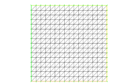
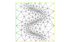
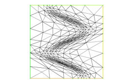
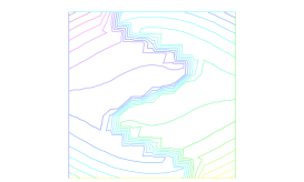
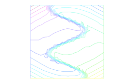
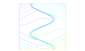
Fig. 2: Interpolation of (13) with ${\rm\hbox{I\kern-1.99997pt\hbox{P}}}_{1}$ elements on a uniform, isotropic or anisotropic mesh of cardinality $500$.

References

• [1] Jean-Marie Mirebeau, Ph.D Thesis, Adaptive and anisotropic finite element approximation : Theory and algorithms, tel.archives-ouvertes.fr/tel-00544243/en/
• [2] FreeFem++ software, developped by Frederic Hecht, www.freefem.org/ff++/