We present a procedure to construct a configuration-interaction expansion containing arbitrary excitations from an underlying full-configuration-interaction-type wave function defined for a very large active space. Our procedure is based on the density-matrix renormalization group (DMRG) algorithm that provides the necessary information in terms of the eigenstates of the reduced density matrices to calculate the coefficient of any basis state in the many-particle Hilbert space. Since the dimension of the Hilbert space scales binomially with the size of the active space, a sophisticated Monte Carlo sampling routine is employed. This sampling algorithm can also construct such configuration-interaction-type wave functions from any other type of tensor network states. The configuration-interaction information obtained serves several purposes. It yields a qualitatively correct description of the molecule’s electronic structure, it allows us to analyze DMRG wave functions converged for the same molecular system but with different parameter sets (e.g., different numbers of active-system (block) states), and it can be considered a balanced reference for the application of a subsequent standard multi-reference configuration-interaction method.

Date:	May 12, 2011
Status:	revised version accepted by J. Chem. Phys.

1 Introduction

In quantum chemistry, electronic wave functions are usually represented as configuration-interaction (CI) expansions, i.e., wave functions expanded in a set of Slater determinants or configuration state functions [1]. The dimension of this many-particle basis, however, grows binomially with the number of orbitals and electrons present in the molecule under study which restricts the application of CI-type methods. In 1990, Olsen, Jørgensen and coworkers managed to perform full CI (FCI) calculations with more than one billion Slater determinants [2].

It was found that CI vectors are actually sparse [3] if contributions below a predefined threshold are neglected. Different approaches have been proposed which take advantage of the sparsity of CI vectors to either overcome the limitations in FCI calculations [4, 5, 6] or to systematically determine only the important configurations in the wave function expansion [7, 8, 9]. In particular, the latter procedures allow a dynamic selection of important configurations without any predefined and limiting excitation scheme applied to a reference configuration [10]. Such methods are, in principle, applicable to any kind of electronic structure. For specific types, like closed-shell electronic structures, special techniques have been developed as powerful and efficient tools like the standard single-reference coupled-cluster (CC) method [1], which generates a predefined CI expansion based on a specific orbital-excitation hierarchy. Still, generally applicable CI methods are sought for difficult cases like for open-shell molecules with a multi-reference character (for which open-shell transition metal clusters are an example [11, 12, 13]) or for excited states.

Such a promising method is the density matrix renormalization group (DMRG) algorithm introduced by White into solid state physics[14, 15]. The DMRG algorithm can be understood as a complete-active-space (CAS) CI method. Compared to most other electron-correlation methods, much larger active spaces can be treated within the DMRG approach without a predefined truncation of the complete $N$-particle Hilbert space. This feature of the algorithm allows one to obtain qualitatively correct wave functions and energies for very difficult electronic structures [16, 17].

The numerical DMRG optimization avoids the application of a predefined analytic CI expansion of the wave function, and hence, no straightforward connection can be established between the DMRG basis states and the linear expansion in terms of Slater determinants. This feature of the algorithm is actually the reason why DMRG can converge CASCI wave functions for very large active spaces, for which an explicit construction of the complete many-particle basis is prohibitive (for an example see Ref. [18]). One might argue that the explicit knowledge of the CI expansion coefficients is not needed as the one- and two-particle density matrices produced by DMRG are sufficient to calculate physical observables. However, detailed information about the underlying wave function should not be disregarded as it can be used for the following purposes.

1. An analysis of DMRG wave functions in terms of CI expansion coefficients will be useful to better understand the quality of the converged DMRG result as the electronic energy is not sufficient as a sole criterion to assess the accuracy obtained [21]. Also for well-established electron-correlation models based on the CC approach Hanrath [53, 54] has observed for the H₄ and HF model systems that considering the energy as the only convergence criterion is not sufficient. Only an analysis of the underlying CC wave function revealed artifacts in the wave function expansion. In other words, in CC calculations one may obtain a wave function expansion that differs notably from an FCI reference although the corresponding CC energy seems to be well converged towards the FCI reference energy. As a consequence, Hanrath and co-workers advocated for a comparison of wave functions rather than energies to assess the quality of a calculation. The same holds true for DMRG wave functions.

2. Since the CI decomposition proposed can be obtained for any converged DMRG calculation, different DMRG calculations can be compared. This is beyond a purely numerical comparison of expectation values and allows one to assess whether qualitatively similar wave functions were actually obtained after DMRG convergence, whose main disadvantage is its purely numerical procedure with convergence properties that are difficult to control and to steer.

3. Accordingly, the CI decomposition may help to optimize DMRG convergence as one can study when and why various electronic configurations are picked up. Reconstructing analytic wave functions facilitates the understanding and analysis of electronic structure in terms of coefficients of Slater determinants. This is hardly possible from the matrix product states (MPS) [19, 20] which is optimized by the DMRG algorithm.

4. A fast DMRG calculation with a small number of renormalized system states, which is always feasible and routinely possible in terms of computer time, may be used to sample important determinants which may then be used as input to a multi-reference CI procedure.

A determinantal analysis of DMRG states has already been presented by our group [21]. The ’transcription’ scheme of DMRG states into a Slater determinant basis used in that work is, however, only applicable to a small number of active orbitals. Larger active spaces containing $L$ spatial orbitals remain computationally unfeasible since all states in the Fock space spanned by these $L$ orbitals were kept. The number of basis states grows, of course, exponentially with the number of orbitals $L$ (e.g., as $4^{L}$ for spatial orbitals). Thus, the fact that DMRG allows us to obtain results for very large active spaces well beyond the binomial scaling wall of common multi-reference methods, i.e., beyond the binomially growing dimension of the complete $N$-particle Hilbert space, which scales as ${\displaystyle L\choose N_{\alpha}}\cdot{\displaystyle L\choose N_{\beta}}$ with ${\displaystyle L\choose N_{\sigma}}=\frac{\displaystyle L!}{\displaystyle N_{\sigma}!(L-N_{\sigma})!}$ for $\sigma\in\{|\uparrow\rangle,|\downarrow\rangle\}$, has not been exploited yet. As a consequence, an improved decomposition scheme is required, which can be employed for any dimension of the active space. So far, the direct calculation of CI coefficients from MPS [19, 20] has not been explicitly carried out for molecular electronic structures and we will show here how this can be accomplished for active spaces larger than those feasible for FCI-type approaches.

This work is organized as follows. In section 2, we present our improved decomposition scheme of the DMRG wave function. Then in section 3, we discuss the sampling routine to explore the binomially large Hilbert space efficiently by means of a Monte Carlo approach, which is then tested at the ozone transition state structure and applied to reconstruct the CI coefficients for a large active space of the Arduengo carbene in section 5. Finally, a summary and concluding remarks are given in section 6.

2 CI expansion of DMRG states

The total DMRG state $\Psi^{(s)}(N)$ describes $N$ electrons at a given DMRG (micro)iteration step $s$ and is given by

$$\Psi^{(s)}(N)=\sum_{ij}\psi_{ij}^{(s)}\left|i\right\rangle\otimes\left|j\right\rangle$$ (1)

with expansion coefficients $\psi^{(s)}_{ij}$. {$\left|i\right\rangle$} and {$\left|j\right\rangle$} represent the orthonormal product basis of the system (also called active subsystem) and the environment (complementary subsystem), respectively. These basis states are never explicitly constructed [22, 21], only the expansion coefficients $\psi^{(s)}_{ij}$ are obtained in each step of the algorithm. We assume a two-site DMRG protocol.

A common expansion of total wave functions employed in quantum chemistry consists of a linear combination of Slater determinants $\Phi_{\{\bf n\}}=|n_{1}\ldots n_{L}\rangle$. Here, $\Phi_{\{\bf n\}}$ is given in its occupation number representation and $\{\bf n\}$ represents the set of all occupation number vectors constructed from $L$ one-particle states. The total DMRG wave function may then be written as a CI-type wave function,

$$\Psi^{(s)}(N)=\sum_{\{\bf n\}}C_{\{\bf n\}}^{(s)}\Phi_{\{\bf n\}},$$ (2)

where the expansion coefficients $C_{\{\bf n\}}^{(s)}$ are the CI coefficients that are to be determined. The sum in Eq. (2) runs over all occupation number vectors in the $N$-particle Hilbert space with the correct particle number, projected spin, and point-group symmetry.

It is important to understand that the two sets of expansion coefficients, $\{\psi_{ij}^{(s)}\}$ and $\{C_{\{\bf n\}}^{(s)}\}$, are not identical, but the CI coefficients $\{C_{\{\bf n\}}^{(s)}\}$ can be reconstructed from the DMRG expansion coefficients $\{\psi_{ij}^{(s)}\}$ and the renormalization matrices [21]. For the explicit reconstruction of CI coefficients for a DMRG wave function, the work of Östlund and Rommer [19, 20] showed that the DMRG algorithm establishes a recursion relation for matrix product states. They considered projection operators $\hat{A}_{i}[n_{i}]$ dependent on the local site $n_{i}$ which map from one $m$-dimensional space spanned by an orthonormal basis {$\left|m_{l-1}\right\rangle$} to another $m$-dimensional space spanned by {$\left|m_{l}\right\rangle$} where $l$ denotes the number of molecular orbitals already incorporated in the active subsystem. These projection operators can be represented by $m\times m$ matrices $({A}_{i}[n_{i}])_{m_{l};m_{l-1}}$. In the renormalization step of the DMRG algorithm the dimension of the product basis of the enlarged system block {$\left|m_{l-1}\right\rangle\otimes\left|n_{l}\right\rangle$} is reduced to a set of new basis states which represent the most important states {$\left|m_{l}\right\rangle$} of the enlarged block,

$$\left|m_{l}\right\rangle=\sum_{m_{l-1},n_{l}}(A_{l}[n_{l}])_{m_{l};{m_{l-1}}}|m_{l-1}\rangle\otimes|n_{l}\rangle,$$ (3)

where the tensor product $\textstyle|m_{l-1}\rangle\otimes|n_{l}\rangle$ is a basis state of the active subsystem. We can now perform a backward recursion to express $\left|m_{l-1}\right\rangle$ through $\left|m_{l-2}\right\rangle$ and so forth, until we reach the first site of the lattice. For a system block of length $l$ we then obtain

$$\left|m_{l}\right\rangle=\sum_{n_{1}\ldots n_{l}}\left(A_{l}[n_{l}]\ldots A_{2}[n_{2}]\right)_{m_{l};n_{1}}|n_{1}\ldots n_{l}\rangle,$$ (4)

with $\left|n_{1}\ldots n_{l}\right\rangle=\left|n_{1}\right\rangle\otimes\left|n_{2}\right\rangle\otimes\ldots\otimes\left|n_{l}\right\rangle$. The DMRG states of the environment block can be expanded in a similar way. Combining Eqs. (4) and (1) and the corresponding recursion relation for the environment states, we can write for the superblock wave function

$$\Psi^{(s)}(N)= \sum_{\{\bf n\}}\sum_{m^{S}}\sum_{m^{E}}\psi_{m^{S}n_{l+1}n_{l+2}m^{E}}^{(s)}$$ (5)

$$\times\left(A_{l}[n_{l}]\ldots A_{2}[n_{2}]\right)_{m^{S};n_{1}}\times\left(A_{l+3}[n_{l+3}]\ldots A_{L-1}[n_{L-1}]\right)_{m^{E};n_{L}}\times\left|n_{1}\ldots n_{L}\right\rangle.$$

for a lattice of length $L$. Hence, the superblock wave function lives in a space spanned by two matrix product states and a product of two local sites [23, 16, 12]. By comparing Eqs. (2) and (5), we can now identify the CI coefficients for the $s$-th microiteration step

$$C_{\{\bf n\}}^{(s)} = \sum_{m^{S}}^{m}\sum_{m^{E}}^{m}\psi_{m^{S}n_{l+1}n_{l+2}m^{E}}^{(s)}$$

$$\times\left(A_{l}[n_{l}]\ldots A_{2}[n_{2}]\right)_{m^{S};n_{1}}\times\left(A_{l+3}[n_{l+3}]\ldots A_{L-1}[n_{L-1}]\right)_{m^{E};n_{L}}.$$

The CI coefficients can be determined for any composition of the lattice blocks as soon as all lattice-position-dependent transformation matrices $A_{j}$ are obtained which are optimized during one sweep of the DMRG algorithm. Note that these transformation matrices are represented as $4m\times m$ matrices in the DMRG algorithm and need to be decomposed into four $m\times m$ matrices for each possible occupation of site $j$ ($|\uparrow\downarrow\rangle,|\downarrow\rangle,|\uparrow\rangle,|\rangle$).

3 Exploring the binomially large many-particle Hilbert space

In the previous section, we have discussed how to calculate CI coefficients for a given occupation number vector within the DMRG framework. It is, however, unfeasible and unnecessary to create the entire basis of the $N$-particle Hilbert space since the numerical evidence compiled over the years demonstrates that only a fraction of the entire set of occupation number vectors is decisive for a sufficiently reliable representation of the wave function [3, 4, 10, 7, 8, 9]. In the language of DMRG, this translates to our previous observations [24, 17] that already small-$m$ DMRG calculations provide accurate and qualitatively correct relative energies between two spin states or two isomers on the same potential energy surface. Note that small-$m$ DMRG calculations can, in principle, also describe non-sparse determinantal wave functions. Actually, coupled cluster and truncated configuration-interaction theories also heavily rely on the fact that determinants following only a certain excitation pattern (i.e., orbital substitution pattern) are included in the wave function and still provide very accurate electronic energies for many molecular systems.

3.1 The SR-CAS algorithm

Because of the formally binomially scaling of many-particle states (determinants) in the $N$-particle Hilbert space, an algorithm is required that is capable of sampling important determinants. The basic idea of the sampling routine is related (but not restricted) to the underlying MPS because the DMRG algorithm locally optimizes the parameter space over the MPS [17]. Hence, a local update in an occupation number vector with a large weight might lead more likely to another occupation number vector with another large weight.

Our sampling routine — inspired by our previous work on the variational optimization of tensor network states [25] and by the work of Sandvik and Vidal [26] — performs an excitation of the type $a_{p_{1}}^{\dagger}a_{q_{1}}a_{p_{2}}^{\dagger}a_{q_{2}}\dots a_{p_{i}}^{\dagger}a_{q_{i}}$ from a predefined reference (usually the Hartree–Fock determinant), where $i$ is a random number between $1$ and $N$ ($p_{j}$, $q_{j}$ are also random numbers in the interval from $1$ to $L$), preserving the number of particles, projected spin, and point-group symmetry. This procedure is capable of sampling the complete FCI space. Each step in our sampling procedure consists of three steps. In the first step, we draw a random number between $1$ and $N$ to determine how many excitations — each represented by an excitation operator $a_{p_{j}}^{\dagger}a_{q_{j}}$ — are performed from a reference determinant (still choosing the Hartree–Fock determinant at the start). For each of these excitations, we generate in the second step two further random numbers within the interval of $1$ and $L$ to determine the spin orbitals of the reference that is to be exchanged by one from the virtual space. In the third step, all excitation operators are applied to the reference determinant which then yields a new trial determinant (occupation number vector).

The coefficient of the trial occupation number vector is then calculated according to Eq. (2) and stored in a hash data structure if it is above a predefined threshold. As we are not interested in all tiny coefficients, we store only the relevant basis states with a coefficient larger than the predefined threshold. The threshold value also prevents a binomial scaling in the dimension of the hash. We have employed a thread-safe hash data structure that allows a massively parallel execution of the sampling routine. In the following we abbreviate the sampling–reconstruction algorithm for FCI-type wave function defined in a complete active orbital space as SR-CAS.

3.2 Completeness measure for accuracy control

In order to extend the search over the entire Hilbert space, we update the reference occupation number vector $\Phi_{\bf n}$ by a new one $\Phi_{\bf m}$ according to the probability

$$p(\Phi_{\bf n}\leftrightarrow\Phi_{\bf m})=\min\left(1,\frac{|C_{\bf m}|^{2}}{|C_{\bf n}|^{2}}\right).$$ (7)

The accuracy and quality of the reconstructed CI-type wave function can be monitored by means of the sum over the squared CI coefficients of the already considered occupation number vectors. For this we define a completeness measure (COM),

$${\rm COM}=1-\sum_{\{\bf n\}}|C_{\{\bf n\}}|^{2}$$ (8)

which quantifies the amount of CI coefficients of occupation number vectors that have not yet been sampled. It must be noted that the COM defines a convenient convergence criterion for the sampling routine as it must converge to zero upon sampling of the full determinant space (covered by the DMRG wave function). As a consequence, it can be employed to estimate the quality of the explicit CI-type wave function obtained and of the expectation values calculated with this wave function. In contrast to common threshold measurements defined for the energy as for instance applied by Buenker and Peyerimhoff [55, 56, 57] in multi-reference CI calculations, COM directly refers to the quality of the reconstructed CI wave function since the reference wave function is known and orthonormal. We should note that our SR-CAS algorithm is considered converged when the actual COM value calculated for the reconstructed CI expansion falls below a predefined threshold. Often we use the same threshold as the one needed in the sampling routine described above, except in cases where it turns out that smaller CI coefficients are important for the predefined threshold of COM.

3.3 Quantum fidelity as a measure for DMRG convergence

A measure to assess the convergence of the DMRG algorithm is highly desirable [42, 47]. Usually, DMRG studies perform several calculations with an increasing number of DMRG system states to verify the convergence of the algorithm. The DMRG energy is then usually taken as the sole convergence criterion. There exist other approaches to execute a DMRG calculation which are based on a dynamic selection of the DMRG system states introduced by Legeza et al. [48, 49]. But even his dynamic block state selection (DBSS) procedure requires several calculations to be carried out as the convergence is also monitored by means of the energy expectation value.

With our SR-CAS algorithm at hand, we can now examine a measure of convergence for a sequence of DMRG calculations that are either performed by increasing the number of DMRG block states $m$ or by the DBSS procedure. This measure is based on the likeness — the fidelity — of two quantum states [50, 51]. Already in 2003, Legeza and Sólyom mentioned the potential application of the fidelity concept within the DMRG framework [52]. The fidelity $F$ between two converged DMRG states is defined as

$$F_{m_{1},m_{2}}=|{\ \langle{\Psi_{m_{1}}^{(s)}}}|{\Psi_{m_{2}}^{(s)}\rangle{}}\ |{}^{2}$$ (9)

where $s$ stands for a given microiteration, e.g., for a specific partitioning of the orbital space among the active and complementary subsystems, $\Psi_{m_{1}}$ and $\Psi_{m_{2}}$ denote two DMRG states obtained for different numbers of DMRG block states, $m_{1}$ and $m_{2}$, respectively. Qualitatively speaking, the quantum fidelity measure expresses the overlap between the two states. It can thus also detect a sign change of the CI coefficients which might not significantly affect the energy at all.

The value of the quantum fidelity measure is obvious for cases in which the energy turns out to be no reliable convergence criterion, because the underlying wave functions differ (as can then be detected by the fidelity $F$). In our previous DMRG study on the decomposition of DMRG basis states into a Slater determinant basis [21], we had already observed that the energy can decrease during DMRG iterations, while the corresponding DMRG wave function was qualitatively wrong when compared to the FCI solution. We should recall from the introduction that similar results have been reported in the literature for CC calculations [53, 54].

It is now important to note that Eq. (9) cannot be straightforwardly evaluated because the DMRG basis states are different for the $m_{1}$ and $m_{2}$ calculations. Hence, a simple scalar product of the two expansion coefficient vectors does not yield the overlap measure. This is solved in our work here. The CASCI-type wave function, which we can now generate with our SR-CAS scheme, allows us to calculate the quantum fidelity defined in Eq. (9).

4 A multireference test molecule

In order to study the performance of our reconstruction procedure, we reconsider the multireference molecule that has already served as a test case in our original determinant decomposition of DMRG states [21] (the structure was taken from Ref. [27] and features one short O–O bond length of 121.1 pm, one long O$\cdots$O bond distance of 240.7 pm and an OOO bond angle of 51.1^∘). The calculation of integrals in the molecular orbital basis was performed in $C_{2v}$ point group symmetry with the Molpro program package [28] employing Dunning’s cc-pVTZ basis set [29, 30]. The DMRG calculations were carried out with our program [31]. As active space, eight electrons correlated in nine orbitals were chosen. Hence, the complete many-particle Hilbert space is spanned by 7’956 Slater determinants.

The transition state energies obtained for different quantum chemical methods are shown in Table I. For increasing $m$, the DMRG transition state energy converges quite fast towards the CASCI reference which is then reproduced for $m=156$ DMRG system states.

Table I: Transition state energies for ozone in a cc-pVTZ basis set for different quantum chemical methods. The active space comprises 8 electrons correlated in 9 orbitals. The Hartree–Fock and CASCI results were taken from Ref. [21].

Method	E/Hartree
HF	$-$224.282 241
CASCI	$-$224.384 301
DMRG($m=48$)	$-$224.384 216
DMRG($m=100$)	$-$224.384 300
DMRG($m=156$)	$-$224.384 301

Since the dimension of the many-particle Hilbert space spanned by these nine orbitals is rather small (only 7’956 Slater determinants), it is possible to determine the CI coefficients for all Slater determinants directly with the Molpro program package [28]. This is advantageous as it allows us to test the efficiency of our SR-CAS Monte Carlo sampling routine. As described before, only Slater determinants are accepted with CI coefficients larger than a predefined threshold. A large threshold implies, of course, that quite many ’unimportant’ configurations will be rejected. In Fig. 1, the transition state energy corresponding to the CASCI-type expansion composed of all sampled configurations is shown for a different number of DMRG system states $m$. As one would expect, for decreasing threshold the approximate transition state energy converges towards the CASCI reference energy for all values of system states $m$. It is obvious that the approximate transition state energy is the lower the larger $m$ is (see, e.g., the inlay in Fig. 1). A threshold of $0.0001$, which results from 1’532 explicitly considered determinants, is sufficient to obtain an accurate CASCI-type wave function expansion for which the transition state energy deviates by 1.371 mHartree (3.6 kJ/mol) from the CASCI reference energy for $m=156$. Whether an energy difference of this order can be tolerated or not depends on the accuracy that is desired. For many relative energies sought in chemistry, like reaction energies in transition metal catalysis [11, 12, 13] or excited states [32, 33, 34, 35], this would be sufficiently accurate. A further decrease by two orders of magnitude to a threshold of $10^{-6}$, which now includes 5’650 explicitly considered determinants, leads to a deviation by 11 $\mu$Hartree (0.029 kJ/mol) from the CASCI reference.

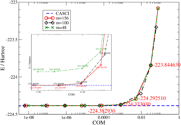
Figure 1: Energy of the ozone molecule in its transition state structure calculated from sampled configurations for different COM values in Hartree. The dashed blue line represents the CASCI reference energy taken from Ref. [21].

The number of Slater determinants which span the sampled subspace of the complete many-particle Hilbert space is shown in Fig. 2. In general, more configurations are needed for larger $m$-calculations in order to reach the desired accuracy, i.e., to fall below a specific threshold, as compared to smaller $m$-calculations. For $m=48$, a kink in the graph can be observed that is not present for larger $m$, which indicates that the DMRG calculation has not incorporated all relevant configurations. Because of these missing configurations, the DMRG algorithm converges to a higher energy for $m$=48 (note that this failure is cured by the DBSS procedure [48, 49]).

As mentioned above, an accurate CASCI-type wave function expansion for $m=156$ is already obtained for a threshold of $0.0001$ which can be expanded in only 1’532 Slater determinants (20% of the complete many-particle Hilbert space). All these Slater determinants correspond to CI coefficients larger than $10^{-4}$. The large percentage of the Hilbert space needed is easy to understand in view of the small active space, which limits the total number of Slater determinants that can be constructed. From a statistical point of view, the ratio of relevant configurations will decrease with increasing dimension of the Hilbert space (i.e., with increasing size of the CAS).

To obtain highly accurate energies in the $\mu$Hartree regime, the threshold can be reduced to $10^{-6}$, where all important configurations are already sampled spanning a subspace consisting of 5’078 Slater determinants (64% of the complete many-particle Hilbert space). The consideration of further ’unimportant’ configurations does not change the corresponding transition state energy (see again inlay in Fig. 1). Note that an accuracy of about 1 kJ/mol in the total electronic energy would require a COM value of about $10^{-5}$. The flattening of the sampling curve when approaching COM $=0$ indicates that only a few configurations are left which have non-zero CI coefficients (but still are much smaller than $10^{-6}$). Hence, the DMRG optimization only picks up the most important configurations and the many-particle Hilbert space is being truncated for $m=48$.

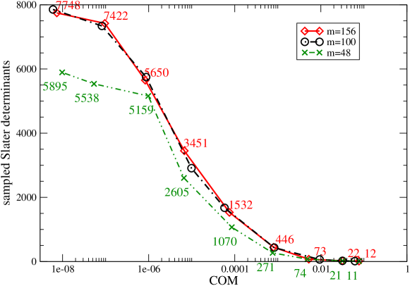
Figure 2: Number of sampled Slater determinants for DMRG calculation employing different $m$ values for the transition state structure of ozone. The total Hilbert space has a dimension of $7^{\prime}956$. A sufficiently accurate wave function can already be obtained for a COM of about $10^{-4}$ which corresponds to 1’532 Slater determinants (about 20% of the complete many-particle Hilbert space.)

A reconstructed analytic CASCI-type wave function can provide further insights into the accuracy of DMRG. Legeza and coworkers [36] speculated that if the accuracy of DMRG calculations is lowered, i.e., if $m$ is decreased, the structure of the wave function will essentially be preserved. This assumption was based on the expectation values, whereas a direct comparison of the wave functions was not performed. With the scheme proposed here, we can now explicitly analyze the dependence of the structure of the CASCI-type wave function expansion on the number of DMRG system states $m$. This can be accomplished by examining the excitation patterns with respect to the configuration with largest CI coefficient for different threshold values and $m$ values which are shown in Fig. 3. Generally, if $m$ is increased, more configurations corresponding to higher excitations are included in the wave function expansion at constant threshold. Exceptions can be observed if more configurations with small CI coefficients are sampled so that in total more Slater determinants are needed to reach the desired threshold for COM. Moreover, by systematically lowering the threshold for the consideration of CI coefficients in the sampling routine, configurations containing higher excitations are picked up (up to octuple excitations) and the maximum of the excitation pattern is shifted towards higher excitations.

The total excitation patterns are similar for all $m$-calculations. We should emphasize that even for $m=48$ octuple excitations are present in the DMRG wave function. In this case with $m=48$, the excitation pattern does not change considerably for a threshold $\leq 10^{-6}$ (see also Fig. 2) and only a few highly excited Slater determinants are picked up. Important higher excitations are missing (too small or zero CI coefficients) in the wave function and the number of DMRG system states $m$ needs to be increased to consider them appropriately. For the fully converged CASCI-type wave function (COM $\leq 10^{-7}$), we observe qualitatively similar excitation patterns for a different number of DMRG system states $m$. In principle, any $n$-fold excitation (heptuple, octuple, …) is accessible by the DMRG algorithm. Most importantly, the total structure of the DMRG wave function is basically retained for different thresholds of accuracy.

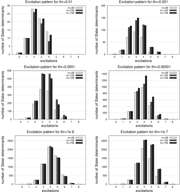
Figure 3: Comparison of excitation patterns with respect to the configuration 110110000000111001 for DMRG calculations on the ozone molecule employing different $m$ values and with respect to a chosen threshold (thr) for the consideration of CI coefficients in the sampling routine. Note the individual scaling of the ordinate for an optimal representation of the excitation spectrum.

Fig. 4 shows the excitation pattern for the DMRG($m=156$) calculation depending on the value chosen for threshold in greater detail. As already mentioned, decreasing the threshold incorporates an increasing number of Slater determinants with a small CI coefficient in the CASCI-type wave function and shifts the maximum of the excitation pattern towards higher excitations. This is due to the fact that higher excitations have smaller CI coefficients and are only sampled if the threshold value is small enough. Note also that our SR-CAS algorithm is capable of picking up the most important configurations first, which correspond to single and double excitations and some triple excitations. To obtain a highly accurate CASCI-type wave function expansion (COM $\leq 0.00001$), higher excitations (mainly quadruple, quintuple and hextuple) must be included as well.

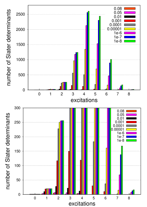
Figure 4: Excitation patterns for the DMRG($m=156$) calculation on the transition state structure of ozone employing different threshold values for the consideration of CI coefficients in the sampling routine. Excitations are given with respect to the 110110000000111001 configuration as reference. The upper graph shows the total excitations spectrum, while the lower half represents a cutout to emphasize the lower and higher excitations, respectively.

The most important CI coefficients are shown in Table II. For an increasing number of DMRG system states $m$, the changes in CI coefficients are small. As the energy still changes notably, this implies that small changes in CI coefficients lead to larger changes in the energy. For $m=156$, the corresponding CI coefficients are in good agreement with the CASCI reference calculation [21].

Table II: CI coefficients of selected configurations of ozone in a transition state structure. The definition of the active space and the labelling of the molecular orbitals were taken from Ref. [21]. Doubly occupied orbitals are denoted as ’2’, empty orbitals as ’0’, and orbitals singly occupied by a spin-up or spin-down electron as ’+’ and ’$-$’, respectively.

Occupation									DMRG			CASCI
$9a^{\prime}$	$10a^{\prime}$	$11a^{\prime}$	$12a^{\prime}$	$13a^{\prime}$	$14a^{\prime}$	$1a^{\prime\prime}$	$2a^{\prime\prime}$	$3a^{\prime\prime}$	$m=48$	$m=100$	$m=156$
2	+	–	0	0	0	2	–	+	0.437 359	0.437 246	0.437 246	0.437 253
2	–	+	0	0	0	2	+	–	0.437 359	0.437 246	0.437 246	0.437 253
2	2	0	0	0	0	2	2	0	0.391 038	0.391 875	0.391 876	0.391 876
2	2	0	0	0	0	2	+	–	0.287 457	0.287 161	0.287 160	0.287 160
2	2	0	0	0	0	2	–	+	0.287 457	0.287 161	0.287 160	0.287 160
2	–	–	0	0	0	2	+	+	0.175 057	0.175 412	0.175 412	0.175 405
2	+	+	0	0	0	2	–	–	0.175 032	0.175 412	0.175 412	0.175 405

To obtain a CASCI-type wave function that yields an accuracy for the energy expectation value of less than 1 kJ/mol compared to the reference energy, a COM of about $10^{-5}$ for the determinant selection in the SR-CAS algorithm is sufficient. Due to the predefined parameters of our SR-CAS algorithm, the reconstructed wave function is a sum over configurations with weights above $10^{-5}$. To demonstrate that this is indeed the case, the relative distribution of CI coefficients with respect to the dimension of the total Hilbert space is plotted in Figure 5. One can observe that the main part of the CASCI wave function consists of configurations with smaller weights ($<10^{-4}$) and that our SR-CAS algorithm is capable of picking up the configurations with largest weights since almost all Slater determinants with CI coefficients larger than $10^{-4}$ have been sampled (compare Figure 5 which shows the relative distribution of CI coefficients for the total Hilbert space).

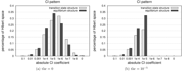
Figure 5: Composition of the total Hilbert space measured in terms of the absolute values of CI coefficients for ozone in its transition state and equilibrium structures. The abscissa refers to configurations with CI weights between the given value (lower bound) and the next higher value on the left (upper bound). The ordinate gives the portion of the configurations considered with respect to the total Hilbert space. (a) Structure of the total Hilbert space. (b) Structure of the sampled configurations for a threshold of $10^{-5}$.

For the multireference case, i.e., for ozone in its transition state structure, our analysis provides an overview on the composition of the Hilbert space in terms of CI coefficient distribution. It is interesting to see how the composition of the Hilbert space and its sampled subspaces change when single-reference systems are considered. The ozone molecule in its equilibrium structure represents such a typical single-reference case. In Figure 5, the distribution of (the absolute values of) CI coefficients for ozone in its transition state are compared to those of the equilibrium structure. The total wave function of the single-reference case is composed of more configurations with larger CI weights ($>10^{-5}$), while for the multi-reference molecule, the maximum of the curve is shifted towards lower-weighted configurations ($<10^{-6}$) than it is observed for the single-reference case. This distribution of CI weights indicates that for single-reference molecules a larger percentage of the Hilbert space needs to be sampled for a given accuracy of the electronic energy and thus to fall below a predefined threshold for COM. To obtain a highly converged wave function (COM $\leq 10^{-5}$), considerably more configurations out of the total Hilbert space are necessary for the ozone molecule in its equilibrium structure than in its transition state structure. Hence, our SR-CAS algorithm has to pick up a larger portion of the Hilbert space if electronic structures with single-reference character are considered. For this reason, we may well choose a single-reference case to study our SR-CAS sampling-reconstruction algorithm as its reliability will strongly depend on its capability to sample the relevant portion of the Hilbert space.

To conduct a proof-of-principle analysis of the fidelity measure at the example of the ozone molecule, we calculate for our three DMRG calculations with $m=48,100,156$ the quantum fidelity. The set of these overlap measures is {$(0.999^{\prime}977^{\prime}5)^{2},(-0.999^{\prime}999^{\prime}9)^{2}$} which indicates that the changes in the wave function are small for increasing $m$. Increasing $m$ from $m=100$ to $m=156$ DMRG block states corresponds to $F_{100,156}=(-0.999^{\prime}999^{\prime}9)^{2}$ which clearly shows the similarity of both DMRG wave functions. Note that the minus sign implies a global sign change in the CI coefficient structure which, of course, does not affect the structure of the wave function since the total wave function can always be multiplied by a factor of $-1$.

5 Reconstructed CI expansion for the Arduengo carbene

In this section, we now study an active space that cannot be treated exactly because of its size. We choose the 1,3-dimethyl Arduengo carbene (see Fig. 6) that was first experimentally characterized in 1992 [37]. Although this molecule is a typical representative of a single-reference molecule and standard coupled-cluster and even Møller–Plesset calculations may yield lower electronic energies, such small aromatic molecules turn out to be rather difficult when their excitation spectra shall be calculated with standard CASSCF-type methods because of the mixture of substituent orbitals with orbitals from the aromatic ring (compared to the unsubstituted imidazole-2-ylidene). As a consequence, the methyl substituents lead to an active space of 16 electrons to be correlated in 28 molecular orbitals in a CASCI- or CASSCF-type approach. Although we do not aim at specific properties of the Arduengo carbene in this work, it is a suitable test case to make the point that we can sample a CAS that is not feasible to study in a CASCI (i.e., FCI) or CASSCF approach.

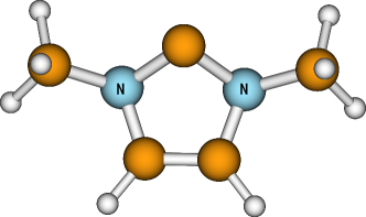
Figure 6: BP86/TZP [44, 45] optimized structure of 1,3-dimethyl imidazole-2-ylidene in its triplet state. The optimization was performed using the quantum chemical program package ADF [46].

We performed DMRG calculations of the triplet state of 1,3-dimethyl-imidazole-2-ylidene with an active space of 16 electrons and 28 orbitals. Hence, this is the first DMRG study to report CI coefficients for an active space that cannot be treated by conventional CAS-type methods, which would span a complete many-particle Hilbert space of dimension $8\times 10^{12}$. The dimension of the DMRG system states was set to $m=60$, 80, 100, and 140 and one DMRG sweep comprises 25 microiteration steps. As orbital basis, natural orbitals from a CASSCF calculation employing an active space of 12 electrons and 12 orbitals [38, 39, 40] were taken. The CASSCF calculations as well as the calculation of the one-electron and two-electron integrals were performed with the Molpro program package [28] using Dunning’s cc-pVTZ basis set for all atoms [29, 30]. We have monitored the CI coefficients during the variational DMRG optimization for the $m=60$ DMRG calculation.

The DMRG ground state energies corresponding to different $m$ values and the CAS(12,12) reference are given in Table III. The DMRG ground state energy decreases systematically for an increasing number of DMRG states $m$. From $m=80$ onwards, the DMRG energy is lower than the CAS(12,12) reference energy as one would expect in view of the larger active space. In this particular case, one may obtain lower electronic energies from a coupled-cluster or Møller–Plesset calculation and therefore we should emphasize that the Arduengo carbene serves simply as an example to explore the CI coefficients of an CASCI-type wave function.

Table III: Ground state energies for the Arduengo carbene in Hartree for CAS(12,12) and DMRG calculations employing a different number $m$ of DMRG basis states.

Method	$E$/Hartree
CAS(12,12)	$-$302.933 197
DMRG($m=60$)	$-$302.930 459
DMRG($m=80$)	$-$302.933 253
DMRG($m=100$)	$-$302.935 120
DMRG($m=140$)	$-$302.937 288

For $m=60$, the DMRG total electronic energy decreases considerably during the first four sweeps of the algorithm, i.e., during the first 100 microiteration steps (see Fig. 7, in which the microiteration steps from 51 to 250 are shown). During these iterations the CI coefficients also change substantially.

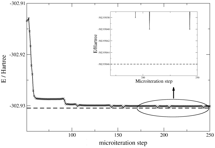
Figure 7: Convergence of the Arduengo-carbene DMRG energy for $m=60$ displayed from the 51^st to the 250^th DMRG($m=60$) microiteration steps. The dashed red line corresponds to the energy of the final converged total state which is reached after 50 sweeps, i.e. 1’250 microiterations.

The convergence behavior of the DMRG energy relates to the convergence of the CI coefficients. To demonstrate this, we depict eight configurations corresponding to CI coefficients with largest weights present in the final ground state wave function for the DMRG ($m=60$) calculation, denoted by SD1 to SD8, where SD1 represents the Hartree–Fock reference configuration. The evolution of the absolute value of the CI coefficients is shown in Fig. 8. The total ground state is dominated by the reference configuration SD1 and contains several configurations with small CI coefficients ($\leq 0.13$). The fast drop in energy during the first ten microiteration steps of the third sweep involves the largest change of CI weights, where more configurations with small CI coefficients are picked up. Afterwards, the DMRG energy reaches a plateau where no changes in CI weights can be observed simultaneously, followed by a second, but smaller decrease in energy at the same partitioning of the orbitals into system and environment as during the first energy jump. Here, another significant change in CI weights can be observed. Then, both the DMRG energy and the CI weights gradually converge to their corresponding final values.

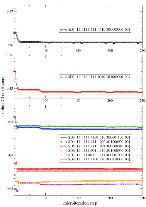
Figure 8: Evolution of the absolute value of the Arduengo-carbene CI coefficients of selected configurations during the DMRG microiteration steps. The binary numbers in the legend correspond to the occupation number vectors in the spin orbital basis. Two consecutive spin orbitals represent one site of the lattice, where the first one corresponds to a spin-up state and the second one to a spin-down state, respectively. Only the first 13 lattice sites are shown, for all other lattice sites the spin orbitals are unoccupied which we abbreviated by {00}.

In Table IV, the CI coefficients corresponding to the eight monitored configurations of the total ground state wave function are shown for different $m$ values. In general, the differences in CI weights for an increasing number of DMRG states $m$ are minor and are up to approximately three orders of magnitude smaller than the reference CI coefficients. It is clear that the electronic structure in such a single-reference case is dominated by the Hartree–Fock determinant and we shall focus on the contribution of the determinants with smaller CI weight. Changes can be observed for SD4 (10%), SD5 and SD6 (both 5%). In particular, the increase in CI weights for larger $m$ exchanges the weighted order of SD3 and SD4, while for all other Slater determinants the ordering stays unchanged. With increasing $m$, the CI weight of the Hartree–Fock reference configuration decreases slightly resulting in larger contributions from different excited configurations. We thus observe that small changes in the CI coefficients induce large changes in energy (7 mHartree).

However, the general pattern of magnitude of the CI coefficients remains similar. Hence, CI coefficients have the same order of magnitude for calculations with different $m$ values. As the CI coefficients do not change considerably when $m$ is increased, it is sufficient to start the sampling for small $m$-DMRG calculations, and then refine the sampled Hilbert space for larger $m$. This makes the sampling procedure more efficient. However, it is obvious that $m$ must not be too small, especially in multi-reference cases.

Table IV: CI coefficients of the total ground state wave function of the Arduengo carbene calculated for different $m$ values. The binary numbers correspond to the occupation number vectors in the spin orbital basis. Two spin orbitals represent one site of the lattice. Only the first 13 lattice sites are shown, for all other lattice sites the spin orbitals are unoccupied which we abbreviated by {00}.

#	SD	$m=60$	$m=80$	$m=100$
1	11111111111111101000000000{00}	0.960 540	0.958 072	0.957 032
2	11111111111100101011000000{00}	0.129 123	0.137 996	0.138 337
3	11111111110011101000001100{00}	0.048 283	0.048 724	0.048 635
4	11111111111110001011000000{00}	0.047 771	0.052 114	0.052 272
5	11111111111110011000000010{00}	0.035 522	0.035 752	0.037 352
6	11111111001111101011000000{00}	0.035 301	0.036 879	0.037 100
7	11111110110111111000001000{00}	0.032 598	0.032 291	0.032 384
8	11111111110011101000110000{00}	0.031 347	0.031 788	0.031 964

We also studied the efficiency of our SR-CAS algorithm for different convergence criteria with respect to the total DMRG ground state. For decreasing COM values the calculated energy for the sampled configurations converges towards the total ground state energy for a given number of DMRG basis states (see Fig. 9). Already for ${\rm COM}=0.000992643$, we capture 99.98% of the ground state energy ($\Delta E=46\rm mH$), while the sampled Hilbert space contains less than 0.94 ppb of the total number of Slater determinants (see also Fig. 10). A further decreasing of the COM to 9.98928$\times 10^{-5}$ captures 99.998% of the total ground state energy ($\Delta E=4.6\rm mH$) in a Hilbert space spanned by only 70’916 Slater determinants (8.67 ppb of the total Hilbert space). Our SR-CAS algorithm is thus capable of capturing the most important configurations of the full Hilbert space while keeping the dimension of the CI-type expansion small.

It would also be interesting to study the number of determinants that needs to be considered for a given accuracy in electronic energy with increasing size of the CAS. This, however, has already been studied by Surján and co-workers who showed that the relative portion of important determinants shrinks with increasing size of the CAS [41], which is an advantage for our SR-CAS algorithm.

In general, we observe that the energy corresponding to the sampled configurations is sensitive to the threshold value chosen. This energy expectation value can serve as an additional convergence criterion. Hence, for an accurate representation of the wave function, the threshold value can be reduced systematically until the desired accuracy of the energy corresponding to the sampled configurations is reached.

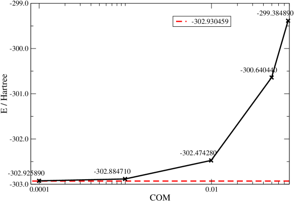
Figure 9: Arduengo-carbene electronic energy corresponding to the sampled configurations for different COM values in Hartree. The dashed red line represents the fully converged DMRG($m=60$) ground state energy.

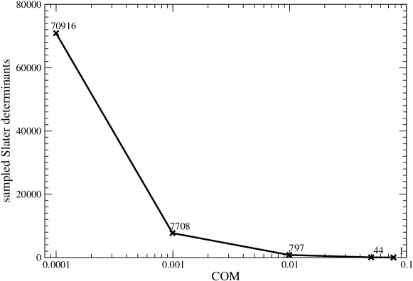
Figure 10: Number of sampled Slater determinants for the DMRG($m=60$) calculation on the Arduengo carbene. The total Hilbert space has a dimension of $8\times 10^{12}$.

6 Conclusions

In this work, we presented a new method for the construction of CASCI-type wave functions for molecular systems comprising a large active space. The first study of a decomposition of DMRG basis states into Slater determinants [21] suffered from an exponential scaling and could therefore be applied to a small active space only. Here, we significantly improved the decomposition scheme by calculating the CI coefficients directly from matrix product states. Thereby, we benefit from the polynomial scaling of the DMRG algorithm so that wave functions of large active spaces can easily be analyzed in terms of the CI language. Since we are in general interested in the final ground or excited state wave function, only the transformation matrices of the last two sweeps of the algorithm need to be stored so that the additional computational cost and memory requirements are negligible. The fact that the complete determinant basis cannot be explicitly constructed for a large CAS necessitates the introduction of the SR-CAS algorithm to pick up all determinants required to achieve a given accuracy in the electronic energy. In turn, this sampling algorithm produces a minimal CI expansion for a desired accuracy, which is surprisingly close to the full DMRG reference energy.

To enhance the efficiency of the sampling in the SR-CAS algorithm, an initial sampling of the full Hilbert space can be performed for a small value $m$ of renormalized DMRG block states. These sampled configurations can then be used as input for large-$m$ calculations as one may expect the CI coefficients to be of similar weight for different dimensions of DMRG system states. Provided that the initial DMRG calculation did not employ a too small value for $m$, this should hold for single- and multi-reference cases. In other words, our procedure exploits the sparsity of large-scale CI problems in a most efficient manner. We have explicitly shown for the Arduengo carbene that only 70’916 out of $8\times 10^{12}$ Slater determinants are necessary for a reliable CI expansion. Our analysis suggests that only a comparatively small number of Slater determinants of the entire $N$-particle Hilbert space has to be considered to construct a very efficient CASCI-type wave function.

Finally, we should emphasize that the presented SR-CAS algorithm can also be used to reconstruct CI-type wave functions for any tensor network state like complete-graph tensor networks [25] and correlator product states [43]. Such a CI-type expansion would facilitate the understanding and analysis of otherwise complicated wave functions.

References

- [1] T. Helgaker, P. Jørgensen, and J. Olsen, Molecular Electronic-Structure Theory, Wiley, 2000.
- [2] J. Olsen, P. Jørgensen, and J. Simons, Chem. Phys. Lett. 169, 463 (1990).
- [3] P. J. Knowles and N. C. Handy, J. Chem. Phys. 91, 2396 (1989).
- [4] P. J. Knowles, Chem. Phys. Lett. 155, 513 (1989).
- [5] R. J. Harrison, J. Chem. Phys. 94, 5021 (1991).
- [6] A. V. Luzanov, A. L. Wulfov, and V. O. Krouglov, Chem. Phys. Lett. 197, 614 (1992).
- [7] A. O. Mitrushenkov, Chem. Phys. Lett. 217, 559 (1994).
- [8] D. Feller, J. Chem. Phys. 98, 7059 (1993).
- [9] J. C. Greer, J. Chem. Phys. 103, 1821 (1995).
- [10] J. C. Greer, J. Comput. Phys. 146, 181 (1998).
- [11] M. Reiher, Chimia 63, 140 (2009).
- [12] K. H. Marti and M. Reiher, Phys. Chem. Chem. Phys. 13, 6750 (2011),
- [13] M. Podewitz, M. T. Stiebritz, and M. Reiher, Faraday Discuss. 148, 119 (2011).
- [14] S. R. White, Phys. Rev. Lett. 69, 2863 (1992).
- [15] S. R. White and R. M. Noack, Phys. Rev. Lett. 68, 3487 (1992).
- [16] G. K.-L. Chan, J. J. Dorando, D. Ghosh, J. Hachmann, E. Neuscamman, H. Wang, and T. Yanai, An Introduction to the Density Matrix Renormalization Group Ansatz in Quantum Chemistry, in Frontiers in Quantum Systems in Chemistry and Physics, edited by S. Wilson, P. J. Grout, J. Maruani, G. Delgado-Barrio, and P. Piecuch, volume 18 of Prog. Theor. Chem. Phys., pages 49–65, Dordrecht, 2008, Springer, arXiv:0711.1398v1 [cond-mat.str-el].
- [17] K. H. Marti and M. Reiher, Z. Phys. Chem. 224, 583 (2010).
- [18] G. K.-L. Chan and M. Head-Gordon, J. Chem. Phys. 118, 8551 (2003).
- [19] S. Östlund and S. Rommer, Phys. Rev. Lett. 75, 3537 (1995).
- [20] S. Rommer and S. Östlund, Phys. Rev. B 55, 2164 (1997).
- [21] G. Moritz and M. Reiher, J. Chem. Phys. 126, 244109 (2007).
- [22] A. O. Mitrushenkov, R. Linguerri, P. Palmieri, and G. Fano, J. Chem. Phys. 119, 4148 (2003).
- [23] U. Schollwöck, Rev. Mod. Phys. 77, 259 (2005).
- [24] K. H. Marti, I. Malkin Ondìk, G. Moritz, and M. Reiher, J. Chem. Phys. 128, 014104 (2008).
- [25] K. H. Marti, B. Bauer, M. Reiher, M. Troyer, and F. Verstraete, New J. Phys. 12, 103008 (2010), arXiv:1004.5303v1 [physics.chem-ph].
- [26] A. W. Sandvik and G. Vidal, Phys. Rev. Lett. 99, 220602 (2007).
- [27] R. Schinke and P. Fleurat-Lessard, J. Chem. Phys. 121, 5789 (2004).
- [28] H.-J. Werner, P. J. Knowles, R. Lindh, F. R. Manby, M. Schütz, P. Celani, T. Korona, A. Mitrushenkov, G. Rauhut, T. B. Adler, R. D. Amos, A. Bernhardsson, A. Berning, D. L. Cooper, M. J. O. Deegan, A. J. Dobbyn, F. Eckert, E. Goll, C. Hampel, G. Hetzer, T. Hrenar, G. Knizia, C. Köppl, Y. Liu, A. W. Lloyd, R. A. Mata, A. J. May, S. J. McNicholas, W. Meyer, M. E. Mura, A. Nicklass, P. Palmieri, K. Pflüger, R. Pitzer, M. Reiher, U. Schumann, H. Stoll, A. J. Stone, R. Tarroni, T. Thorsteinsson, M. Wang and A. Wolf, Molpro, version 2009.1, a package of ab initio programs, 2009, see http://www.molpro.net.
- [29] J. T. H. Dunning, J. Chem. Phys. 90, 1007 (1989).
- [30] N. B. Balabanov and K. A. Peterson, J. Chem. Phys. 123, 064107 (2005).
- [31] G. Moritz, K. H. Marti, K. Boguslawski, and M. Reiher, Qc-Dmrg-ETH, A Program for Quantum Chemical DMRG Calculations. Copyright 2007–2010, ETH Zürich.
- [32] A. Dreuw and M. Head-Gordon, Chem. Rev. 105, 4009 (2005).
- [33] A. Dreuw, ChemPhysChem 7, 2259 (2006).
- [34] J. Neugebauer, Phys. Rep. 489, 1 (2010).
- [35] J. Neugebauer, Orbital-Free Embedding Calculations of Electronic Spectra, in Recent Advances in Orbital-Free Density Functional Theory, page in press, World Scientific, Singapore, 2011.
- [36] Ö. Legeza, J. Röder, and B. A. Hess, Mol. Phys. 101, 2019 (2003).
- [37] A. J. Arduengo, H. V. R. Dias, R. L. Harlow, and M. Kline, J. Am. Chem. Soc. 114, 5530 (1992).
- [38] H.-J. Werner and W. Meyer, J. Chem. Phys. 74, 5794 (1981).
- [39] H.-J. Werner and P. J. Knowles, J. Chem. Phys. 82, 5053 (1985).
- [40] P. J. Knowles and H.-J. Werner, Chem. Phys. Lett. 115, 259 (1985).
- [41] Z. Rolik, Á. Szabados, and P. R. Surján, J. Chem. Phys. 128, 144101 (2008).
- [42] K. H. Marti and M. Reiher, Mol. Phys. 108, 501 (2010).
- [43] H. Changlani, J. Kinder, C. Umrigar, and G. Chan, arXiv:0907.4646v1 .
- [44] J. P. Perdew, Phys. Rev. B 33, 8822 (1986).
- [45] A. D. Becke, Phys. Rev. A 38, 3098 (1988).
- [46] G. T. Velde, F. M. Bickelhaupt, E. J. Baerends, C. F. Guerra, S. J. A. Van Gisbergen, J. G. Snijders, and T. Ziegler, J. Comput. Chem. 22, 931 (2001), see http://www.scm.com.
- [47] K. H. Marti, New Electron Correlation Theories and Haptic Exploration of Molecular Systems, PhD thesis, ETH Zürich, 2010.
- [48] Ö. Legeza, J. Röder, and B. A. Hess, Phys. Rev. B 67, 125114 (2003).
- [49] Ö. Legeza and J. Sólyom, Phys. Rev. B 70, 205118 (2004).
- [50] A. Peres, Phys. Rev. A 30, 1610 (1984).
- [51] H.-Q. Zhou, R. Orus, and G. Vidal, Phys. Rev. Lett. 100, 080601 (2008).
- [52] Ö. Legeza and J. Sólyom, Phys. Rev. B 68, 195116 (2003).
- [53] M. Hanrath, Chem. Phys. Lett. 466, 240 (2008).
- [54] A. Engels-Putzka and M. Hanrath, J. Mol. Struct.: THEOCHEM 902, 59 (2009).
- [55] R. J. Buenker and S. D. Peyerimhoff, Theoret. Chim. Acta 35, 33 (1974).
- [56] R. J. Buenker and S. D. Peyerimhoff, Theoret. Chim. Acta 39, 217 (1975).
- [57] R. J. Buenker, S. D. Peyerimhoff, and W. Butscher, Mol. Phys. 35, 771 (1977).