From entanglement renormalisation to the disentanglement of quantum double models

Abstract

We describe how the entanglement renormalisation approach to topological lattice systems leads to a general procedure for treating the whole spectrum of these models, in which the Hamiltonian is gradually simplified along a parallel simplification of the connectivity of the lattice. We consider the case of Kitaev’s quantum double models, both Abelian and non-Abelian, and we obtain a rederivation of the known map of the toric code to two Ising chains; we pay particular attention to the non-Abelian models and discuss their space of states on the torus. Ultimately, the construction is universal for such models and its essential feature, the lattice simplification, may point towards a renormalisation of the metric in continuum theories.

NSF-KITP-10-163

Keywords: Topological lattice models, tensor networks.

1 Introduction

The application of tensor network methods has provided deep insight into topologically ordered systems. Tensor networks provide a setting where the exotic characteristics of topological order (topology dependent ground level degeneracy, local indistinguishability of ground states, topological entanglement entropy, interplay with renormalisation, unusual realisation of symmetries) can be exactly studied. On the other hand, tensor network methods are sufficiently flexible for studying the excitations of these systems; in 2D, as is known, the excitations are quasiparticles with anyonic exchange statistics, which is the basis of Kitaev’s topological quantum computer architecture [1].

Among lattice models with topological order, Kitaev’s quantum double models [1] have a distinguished position. They were the first models in which the possibilities of the topological setting for quantum computation purposes were discussed, and include anyon models universal for quantum computation by braiding; on the other hand, quantum double models bear an intimate relation to discrete gauge theories, exhibiting a rich group-theoretical and algebraic structure that pervades the study of their ground level and excitations, and in particular determines the properties of the anyons and their computational power. While they are not as general as string-net models [2], the models that describe all doubled topological fixed points on the lattice, steps towards a reformulation of the latter in the spirit of quantum double models have been taken in [3, 4, 5]. Recent progress in the perturbative production of quantum double codes via two-body interactions has been reported in [6].

Tensor network methods were first applied to topological models on the lattice in [7], where an exact projected entangled-pair state (PEPS) representation of a ground state of the toric code was given. In recent years, a growing number of tensor network representations for topological states have been developed following the lead of [7] (e.g. [8, 9, 10, 11, 4]), which are notably exact for ground states of fixed-point Hamiltonians (quantum doubles, string-nets), and moreover lend themselves to deep analysis of their symmetries [12]. Tensor network methods for systems with anyonic quasiparticles, independent of any microscopic structure, have also been developed [13, 14].

The multi-scale entanglement renormalisation ansatz (MERA) is a particular kind of tensor network structure, developed by G. Vidal [15, 16], which builds on the coarse-graining procedure typical for real-space renormalisation flows, but introduces layers of unitary operators between coarse-graining steps so as to reduce interblock entanglement, a procedure called entanglement renormalisation (ER). In practice, ER led to tractable MERA representations and algorithms for ground states of critical systems in 1D, traditionally hard for tensor network methods, and the numerical applications of the method now encompass a wide class of lattice and condensed-matter models both in 1D and in higher dimensions. ER was first applied to topological lattice models in [8], where exact MERAs were given for ground states of quantum double models, both Abelian and non-Abelian. In [9] ground states of string-net models were also written in MERA form.

While understanding ground states of many-body quantum systems is certainly of the utmost importance, it is a bonus for a method to be able to explore at least the low-lying excitation spectrum. The purpose of this paper is to show how the principles of the ER approach to quantum double models can be extended to account for the whole spectrum in an exact way. The picture that emerges is somehow complementary to entanglement renormalisation: by giving up the coarse-graining, that is, using unitary tensors throughout, the ER method turns into a reorganisation of degrees of freedom which is essentially graph-theoretical and proceeds by modifying the lattice by keeping the topological Hamiltonian the same at each step; this procedure yields finally a Hamiltonian consisting essentially of one-body terms, or an essentially classical one-dimensional spin chain model.

Naturally, the structure of the tensor network with unitary operations defines a unitary quantum circuit, which in this case simplifies the structure of the Hamiltonian down to mostly one-body terms. In this sense, the construction can be regarded as an instance of the broad idea of quantum circuits diagonalising Hamiltonians, introduced in [17].

In this vein, we obtain an explicit (and geometrically appealing) construction of the well known mapping of the toric code to two classical Ising chains; but we also cover the non-Abelian cases. Remarkably, the construction is virtually universal for all quantum double models, and can be understood as a series of moves simplifying the structure of the lattice into a series of ‘bubbles’ and ‘spikes’, each one of which talks only to one qudit; each quantum double model possesses a canonical set of operations transforming the model on one lattice into the same model on the next lattice. Since the lattice structure can be considered as the discretisation of a metric, this might open the door to speculations about a continuum counterpart (including, perhaps, dimensional reduction in going from the topological Hamiltonian in 2D to one-dimensional classical chains). We remark that the recent paper [18] uses related ideas to find numerical methods applicable to lattice gauge theories.

The structure of the paper is as follows. The Abelian case of the toric code is discussed in section 2, where we recall the basic elements of the construction of [8], and proceed to a detailed presentation of the disentangling method. In section 3, the analogous construction is developed for general quantum double models; particular attention is given to the models on the torus, where the structure of the Hilbert space has to be taken into account carefully. Section 4 contains a discussion and conclusions. In appendix A some algebraic background underlying quantum double models is provided, and appendix B concentrates on the simplest non-Abelian quantum double, that of the group $\mathrm{S}_{3}$.

2 Entanglement renormalisation of the toric code

We begin by describing the construction in the simplest Abelian case, namely the toric code. This will allow us to make a connection with known results, namely the mapping to a pair of classical Ising chains.

2.1 Elementary moves for the toric code

We start from an arbitrary two-dimensional lattice $\Lambda$, with qubits sitting at the bonds. We do not specify the topology yet. The Hamiltonian, to begin with, has the familiar form of Kitaev’s toric code [1]:

$$H_{\Lambda}=-\,\sum_{P}B_{P}-\,\sum_{V}A_{V}\;,$$ (1)

with

$$B_{P}=\bigotimes_{i\in P}Z_{i}\;,\quad A_{V}=\bigotimes_{j\in V}X_{j}$$ (2)

mutually commuting stabilisers with support on plaquettes $P$ and vertices $V$. Any code state $\lvert\psi\rangle$ (i.e., any ground state of $H_{\Lambda}$) satisfies the local conditions $B_{P}\lvert\psi\rangle=\lvert\psi\rangle$, $A_{V}\lvert\psi\rangle=\lvert\psi\rangle$ for all $P$, $V$; whatever information it carries is purely topological, encoded in the eigenvalues of nonlocal operators.

The entanglement renormalisation scheme proposed in [8] uses two kinds of elementary operations introduced in [19], the plaquette move and the vertex move. In that work only code states were considered, and the result of applying elementary moves was to decouple qubits from the code in known states. More precisely, plaquette moves (P-moves) decouple a qubit $q$ from the lattice by putting it in a product state $\lvert 0\rangle$ with the rest of the system:

$$\lvert\text{code state; $w$}\rangle_{\Lambda}\stackrel{{\scriptstyle P}}{{\mapsto}}\lvert\text{code state; $w$}\rangle_{\Lambda^{\prime}}\otimes\lvert 0\rangle_{q}\;,$$ (3)

where $\Lambda^{\prime}$ is the lattice resulting from the deletion of the edge containing $q$, therefore fusing the two plaquettes to which $q$ belonged into one plaquette. Here $w$ stands for any nonlocal information in the code state, which is preserved provided the plaquette move is purely a bulk operation, that is, it acts on a contractible region. Vertex moves (V-moves) effect a similar simplification,

$$\lvert\text{code state; $w$}\rangle_{\Lambda}\stackrel{{\scriptstyle V}}{{\mapsto}}\lvert\text{code state; $w$}\rangle_{\Lambda^{\prime\prime}}\otimes\lvert+\rangle_{q}\;,$$ (4)

with $\Lambda^{\prime\prime}$ obtained by contracting the edge containing $q$ into a vertex (subsuming the two vertices of the contracted edge). In both cases the topological information carried by the code state is unchanged, if the moves have support on a contractible region.

The programme of entanglement renormalisation can be carried out explicitly and exactly for the code states, as shown in [8], using P-moves and V-moves organised into disentanglers and isometries (in the latter case the decoupled qubits being discarded from the system). This gives rise to an exact MERA ansatz for the code states, whereby the top of the tensor network contains only topological degrees of freedom; for instance, in the case on the torus, these topological degrees of freedom are two qubits on edges along noncontractible loops of $\mathrm{T}^{2}$.

Let us consider more in detail a P-move $U_{\mathrm{plaq}}$ (figure 1, left).

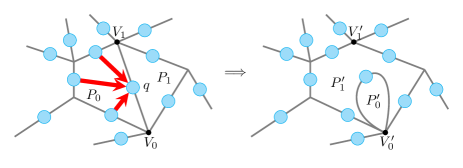
Figure 1: Deformation of the lattice after a P-move. The P-move consists of CNOTs (red arrows). Qubit $q$ “decouples” if in the ground state, but the complete picture is that it remains in the deformed lattice, with its own plaquette (a bubble containing the flux initially in the left subplaquette). To be consistent with the non-Abelian generalisation to be discussed later on, the bubble is attached to one of the vertices talking to $q$.

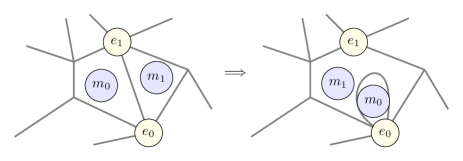
Figure 2: Charges under a P-move. Redistribution of electric charges $e_{i}$ and magnetic fluxes $m_{i}$ in the P-move of figure 1. Note that the redistribution would be different (swapping fluxes $m_{0}$, $m_{1}$ in the deformed lattice) if the control qubits there belonged to the plaquette $P_{1}$, although for the ground states the effect is the same. Each deformed vertex contains the same electric charge as its undeformed predecessor.

This consists of simultaneous CNOTs with target qubit $q$ and control qubits in the remaining edges around one of the two plaquettes $P_{0}$, $P_{1}$ containing $q$ (say, $P_{0}$). Call $P$ the plaquette obtained from $P_{0}$ and $P_{1}$ by deleting the bond for $q$. Only four terms in the Hamiltonian change:

$$U_{\mathrm{plaq}}(B_{P_{0}}+B_{P_{1}}+A_{V_{0}}+A_{V_{1}})U_{\mathrm{plaq}}^{\dagger}=Z_{q}+Z_{q}B_{P}+A_{V^{\prime}_{0}}+A_{V^{\prime}_{1}}\;,$$ (5)

where vertices $V_{0}$ and $V_{1}$ talk to qubit $q$, and $V^{\prime}_{0}$, $V^{\prime}_{1}$ are the new vertices after deletion of the bond containing $q$.

But this calls for a more general interpretation than just the coarse-graining (3) of the ground level. The first term in the rhs of (5) describes qubit $q$ having eaten the flux in plaquette $P_{0}$, but not otherwise subject to vertex constraints; the second term contains all qubits in $P_{0}$ and $P_{1}$, including $q$ counted once, so the new Hamiltonian is not a toric code with $q$ removed, but a toric code with a deformation of the lattice still containing $q$ in a bubble, i.e., in its own plaquette $P^{\prime}_{0}$ contributing to the total flux (figure 1, right). Note that we draw $P^{\prime}_{0}$ attached to one of the vertices of the bond previously containing $q$; this is needed for a consistent generalisation to non-Abelian cases. At any rate, $q$ is not subject to any vertex constraint since it talks twice to this vertex $V^{\prime}_{0}$, and $X^{2}=1$.

The effect of the P-move in terms of charges and fluxes is drawn in figure 2. The electric charges remain at their vertices, while the bubble $P^{\prime}_{0}$ of $q$ contains the flux across $P_{0}$, and the complementary new plaquette $P^{\prime}_{1}$ contains the flux previously in $P_{1}$. Note that while the effect on the ground level is symmetric with respect to the choice of control qubits, this is not the case when there are nontrivial fluxes.

Note also that the total charge and flux of the entire region affected by the local operation $U_{\mathrm{plaq}}$ are conserved, as they should be.

Elementary V-moves are entirely dual to P-moves in the toric code (and, more generally, in any Abelian quantum double model). To be precise, the duality is established by going over to the dual lattice and performing a global Hadamard, thus swapping $X$ and $Z$ operators.

Figure 3 shows the effect of such a move, $U_{\mathrm{vert}}$. The operation consists of CNOTs with the control qubit $q$ in the bond from vertex $V_{0}$ to $V_{1}$ (the one to ‘decouple’ in state $\lvert+\rangle$ if in a ground state) and targets those sharing with $q$ one of the vertices, say $V_{0}$. The result is that the Hamiltonian is mapped to the Hamiltonian of a lattice where the bond of $q$ has been contracted, identifying its two vertices into a new vertex $V^{\prime}_{1}$, to which is attached a ‘spike’, i.e., a bond, containing $q$, whose other vertex $V^{\prime}_{0}$ is not connected to any other bonds. As shown in figure 4, the fluxes in the new plaquettes $P^{\prime}_{0}$ and $P^{\prime}_{1}$ are inherited from those in $P_{0}$ and $P_{1}$, while the electric charge at vertex $V^{\prime}_{0}$ contains the charge previously at vertex $V_{0}$, and the vertex $V^{\prime}_{1}$ at the end of the spike contains the charge of $V_{1}$.

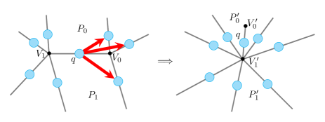
Figure 3: Deformation of the lattice after a V-move. As before, red arrows stand for CNOTs. Qubit $q$ belongs, after the operation, to a spike (a bond with one of its vertices not connected to any other bond).

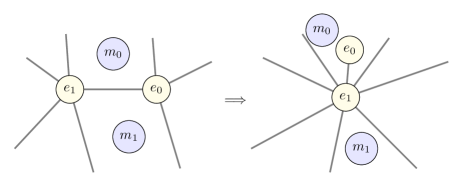
Figure 4: Charges under a V-move. Redistribution of charges and fluxes in a V-move. Again, note that this is not symmetric in the vertices. Had the CNOTs in figure 3 acted on the qubits surrounding $V_{1}$, the electric charges $e_{0}$, $e_{1}$ in the deformed lattice would have been swapped.

2.2 Disentangling the Hamiltonian: a simple example

With the set of elementary moves at hand, we can disentangle the Hamiltonian by simplifying the structure of the lattice.

Think of a toric lattice, to be specific an $L_{x}\times L_{y}$ square lattice $\Lambda_{0}$ with periodic boundary conditions, on which a toric code $\mathrm{\mathbf{TC}}(\Lambda_{0})$ is defined. By using P-moves and V-moves as described in the previous section, the lattice gets deformed into a sequence of lattices $\Lambda_{n}$, $n=1,\,2,\,\ldots$, with the same number of vertices, edges, and plaquettes, and hence the same topology, but increasingly simpler connectivity, and keeping the lattice system a toric code $\mathrm{\mathbf{TC}}(\Lambda_{n})$ at each step. States flow in this process just by redistributing the charges and fluxes.

The lattice can be simplified to reach a particularly appealing form, to which corresponds a Hamiltonian consisting of three sectors:

• A trivial sector corresponding to two qubits encoding the topological degrees of freedom.

• An Ising chain of $L_{x}L_{y}-1$ qubits encoding the structure of magnetic (plaquette) fluxes.

• An Ising chain of $L_{x}L_{y}-1$ qubits encoding the structure of electric (vertex) charges.

To understand this, note that the minimal toric square lattice consists of two links along two nonequivalent nontrivial loops on $\mathrm{T}^{2}$, beginning and ending at a unique vertex, and defining a unique plaquette. In this minimal case, the Kitaev Hamiltonian is trivial and all computational basis states are Kitaev logical states, there being no room for excitations in the Hilbert space.

On performing P-moves and V-moves, the topology of the lattice is left unchanged, but the number of nontrivial cycles along links in the lattice can be reduced to the minimal case, whereby two qubits carry all topological information. Information about excitations in the original lattice will appear in the rest of the code qubits.

Let us illustrate the simplification in the case of a toric lattice with four plaquettes and four vertices. The steps are depicted in figure 5.

Figure 5: Simplification of the lattice for a $2\times 2$ toric code. The end lattice features two topologically nontrivial links and a series of bubbles and spikes, all attached to the same vertex. We have kept qubits in their places and only deformed the lattice links. Red arrows stand for CNOTs and point from control to target qubits. Dark qubits are those that hold a full qubit of topological information. Other colours are used for qubits that hold the flux (medium dark) or charge (light) of a plaquette or vertex of the original lattice.

We consider a basis state of the Hilbert space determined by magnetic fluxes $m_{ij}$ for plaquettes $\mathrm{p}_{ij}$ and electric charges $e_{ij}$ at vertices $\mathrm{v}_{ij}$, taking values in $\{\pm 1\}$ (being the eigenvalues of the corresponding plaquette or vertex operator). Indices $i,\,j$ run from 1 to 2 labelling the horizontal and vertical logical coordinates of the plaquettes and vertices. By overall charge neutrality, $\prod_{ij}m_{ij}=+1=\prod_{ij}e_{ij}$. Topological information is encoded in two nonequivalent nontrivial loops, the eigenvalues of the corresponding logical $Z$ operators being $z_{\mathrm{H}}$, $z_{\mathrm{V}}$. After a series of P-moves and V-moves, the topological data are carried by the two qubits shown in dark in figure 5, which will be denoted as $q_{V,\,H}$. Qubits carrying magnetic information will be referred to as $q_{M,\,i}$, $i=1,\,2,\,3$, and are those whose links enclose a solitary plaquette. Qubits carrying electric information are shown in light colour in figure 5, will be denoted as $q_{E,\,i}$, $i=1,\,2,\,3$, and are those whose link has a free vertex. The final Hamiltonian is

$$H_{\text{final}} =-\,\sum_{i=1}^{3}Z(q_{M,\,i})-Z(q_{M,\,1})Z(q_{M,\,2})Z(q_{M,\,3})$$

$$\quad-\,\sum_{i=1}^{3}X(q_{E,\,i})-X(q_{E,\,1})X(q_{E,\,2})X(q_{E,\,3})\;.$$ (6)

The precise redistribution of fluxes and charges will be discussed in general later, but for the moment let us remark that, as promised, there are no terms in $H_{\text{final}}$ associated with $q_{V,\,H}$, and that the magnetic sector (terms affecting the $q_{M,\,i}$, i.e., involving $Z$s) and the electric sector (terms affecting the $q_{E,\,i})$, i.e., involving $X$s) are each intimately related to an Ising chain Hamiltonian. A cleaner illustration of the lattice structure associated with Hamiltonian (2.2) is given in figure 6 (the Abelian nature of the code allows for generous rearrangement of bubbles and spikes).

Figure 6: A clearer picture of the disentangled $2\times 2$ toric code. Light qubits carry electric information, medium dark qubits carry magnetic information, and dark qubits carry topological information. The Hamiltonian for this code is (2.2).

The correspondence with the Ising chains can be made explicit by especially simple P-moves and V-moves acting on the configuration of figure 6 by direct application of stabiliser formalism results. These are shown in figure 7.

Figure 7: From the disentangled toric code to Ising chains. The sequence of steps to bring the lattice explicitly to the form where the toric code Hamiltonian is the sum (2.2) of two noninteracting Ising chains. Red arrows, as usual, stand for CNOTs.

Denote as $\mathcal{C}(t\leftarrow c)$ the CNOT operation with control $c$ and target $t$. Starting from (2.2), the corresponding operation is

$$\mathcal{C}(q_{E,2}\leftarrow q_{E,1})\mathcal{C}(q_{E,3}\leftarrow q_{E,2})\mathcal{C}(q_{M,3}\leftarrow q_{M,2})\mathcal{C}(q_{M,2}\leftarrow q_{M,1})\;,$$ (7)

whose application yields the doubled Ising Hamiltonian:

$$H_{\text{final}} =-\,Z(q_{M,\,1})-\,Z(q_{M,\,1})Z(q_{M,\,2})-\,Z(q_{M,\,2})Z(q_{M,\,3})-\,Z(q_{M,\,3})$$

$$\quad-\,X(q_{E,\,1})-\,X(q_{E,\,1})X(q_{E,\,2})-\,X(q_{E,\,2})X(q_{E,\,3})-\,X(q_{E,\,3})\;.$$ (8)

2.3 Disentangling the Hamiltonian: full structure

As for the explicit moves and redistribution of charges and fluxes, necessary to understand the unravelling of the Hamiltonian in general, consider an $L\times T$ toric square lattice as shown in figure 8.

Figure 8: General toric code simplification: setting. The starting point for the discussion of the full structure of the procedure of simplification of the toric code. Here qubits are split into two groups according to whether they belong to a horizontal bond ($\mathrm{qh}_{i,j}$) or a vertical bond ($\mathrm{qv}_{i,j}$) in the original $L\times T$ toric lattice. Electric charges $e_{ij}=\pm 1$ at the vertices and magnetic fluxes $m_{ij}=\pm 1$ across the plaquettes are labelled as well by obvious row and column indices, $i=0,\,1,\,\ldots,\,L-1$ and $j=0,\,1,\,\ldots,\,T-1$. Overall charge neutrality on the torus means $\prod_{ij}m_{ij}=1=\prod_{ij}e_{ij}$.

We label vertices according to their coordinates as $\mathrm{v}_{ij}$, where $i$ runs from $0$ to $L-1$ and $j$ runs from $0$ to $T-1$. Plaquette $\mathrm{p}_{ij}$ has vertex $\mathrm{v}_{ij}$ as its lower left corner. Qubits in horizontal links are denoted $\mathrm{qh}_{ij}$, with vertex $\mathrm{v}_{ij}$ to their left, and qubits in vertical links as $\mathrm{qv}_{ij}$, pointing upwards from vertex $\mathrm{v}_{ij}$.

Consider the basis of simultaneous eigenstates of the set of all plaquette operators (eigenvalues $m_{ij}$ with $\prod_{ij}m_{ij}=1$) and vertex operators (eigenvalues $e_{ij}$ with $\prod_{ij}e_{ij}=1$), together with logical $Z$ operators $Z_{H}=\prod_{i=0}^{L-1}Z_{\mathrm{qh}_{i,0}}$ (eigenvalue $z_{H}$) and $Z_{V}=\prod_{j=0}^{T-1}Z_{\mathrm{qv}_{0,j}}$ (eigenvalue $z_{V}$).

The process of simplification of the lattice will be described by the P-moves and V-moves applied to a basis state to bring the lattice to a form generalising figure 6, and the identification of the qubits carrying the eigenvalue of each vertex, plaquette, and logical original operator at that stage.

There is a huge amount of freedom in the choice of the process. I will be describing one possible choice, not optimal in any sense, but allowing a systematic treatment.

Step 1: Create bubbles along rows

Figure 9.

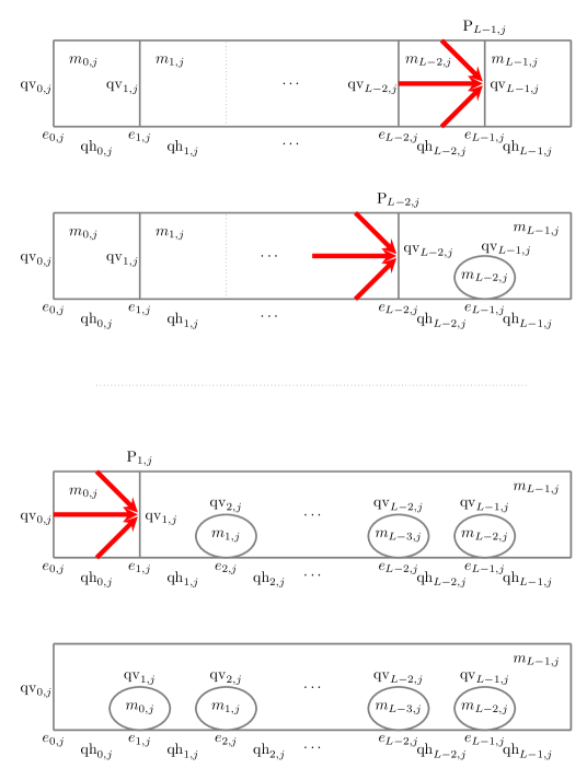
Figure 9: General toric code simplification, step 1. Creating bubbles along each row by P-moves from right to left.

Operation $\mathcal{U}_{1}=\bigotimes_{j=0}^{T-1}U^{\text{row (1)}}_{j}$, with $U^{\text{row (1)}}_{j}=\mathrm{P}_{1,\,j}\mathrm{P}_{2,\,j}\ldots\mathrm{P}_{L-1,\,j}$. P-move $\mathrm{P}_{i,\,j}$ is defined as the application of CNOTs on target qubit $\mathrm{qv}_{i,\,j}$ with controls the rest of the qubits of plaquette $\mathrm{p}_{i-1,\,j}$. Explicitly,

$$\mathrm{P}_{i,j}=\mathcal{C}(\mathrm{qv}_{i,j}\leftarrow\mathrm{qh}_{i-1,\,j+1})\mathcal{C}(\mathrm{qv}_{i,j}\leftarrow\mathrm{qv}_{i-1,\,j})\mathcal{C}(\mathrm{qv}_{i,j}\leftarrow\mathrm{qh}_{i-1,\,j})\;.$$ (9)

Step 2: Create spikes along rows

Figure 10.

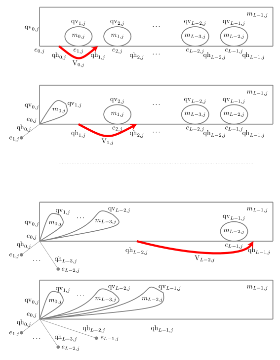
Figure 10: General toric code simplification, step 2. Creating spikes along each row by V-moves from left to right.

Operation $\mathcal{U}_{2}=\bigotimes_{j=0}^{T-1}U^{\text{row (2)}}_{j}$, with $U^{\text{row (2)}}_{j}=\mathrm{V}_{L-2,\,j}\mathrm{V}_{L-3,\,j}\ldots\mathrm{V}_{0,\,j}$. Each V-move here consists of a single CNOT, $\mathrm{V}_{i,\,j}=\mathcal{C}(\mathrm{qh}_{i+1,j}\leftarrow\mathrm{qh}_{i,\,j})$, since the qubit in the affected bubble ($\mathrm{qv}_{i+1,\,j}$) is acted upon twice, and hence unchanged.

At this stage, the toric lattice has been simplified to a single column, to the vertices of which are attached a collection of bubbles and spikes. The next moves reproduce the strategy followed before for each row.

Step 3: Create bubbles along the column

Figure 11.

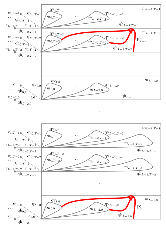
Figure 11: General toric code simplification, step 3. Creating bubbles along the remaining column by P-moves from top to bottom.

Operation $\mathcal{U}_{3}=\mathrm{P}^{\prime}_{0}\ldots\mathrm{P}^{\prime}_{T-2}$, where each P-move consists now of $L$ CNOTs,

$$\mathrm{P}^{\prime}_{j} =\mathcal{C}(\mathrm{qh}_{L-1,\,j+1}\leftarrow\mathrm{qv}_{1,\,j})\ldots$$

$$\quad\times\mathcal{C}(\mathrm{qh}_{L-1,\,j+1}\leftarrow\mathrm{qv}_{L-1,\,j})\mathcal{C}(\mathrm{qh}_{L-1,\,j+1}\leftarrow\mathrm{qh}_{L-1,\,j})\;.$$ (10)

Step 4: Create spikes along the column

Figure 12.

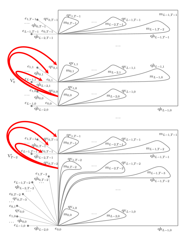
Figure 12: General toric code simplification, step 4. Creating spikes along the column by V-moves from bottom to top.

Operation $\mathcal{U}_{4}=\mathrm{V}^{\prime}_{T-2}\ldots\mathrm{V}^{\prime}_{0}$, where each V-move consists now of $L$ CNOTs,

$$\mathrm{V}^{\prime}_{j}=\mathcal{C}(\mathrm{qh}_{L-2,\,j+1}\leftarrow\mathrm{qv}_{0,\,j})\ldots\mathcal{C}(\mathrm{qh}_{0,\,j+1}\leftarrow\mathrm{qv}_{0,\,j})\mathcal{C}(\mathrm{qv}_{0,\,j+1}\leftarrow\mathrm{qv}_{0,\,j})\;.$$ (11)

After this set of operations, the topological information is carried by qubits $\mathrm{qh}_{L-1,\,0}$ (eigenvalue $z_{H}$) and $\mathrm{qv}_{0,\,T-1}$ (eigenvalue $z_{V}$). All magnetic fluxes in the original plaquettes except for $m_{L-1,\,T-1}$ are now located in one-qubit bubbles, according to the rule

flux $$m_{i,\,j} \mathrm{qv}_{i+1,\,j} 0\leq i\leq L-2 \forall j$$ is carried by qubit , , ,

flux $$m_{L-1,\,j} \mathrm{qh}_{L-1,\,j+1} \forall j$$ is carried by qubit , . (12)

Flux $m_{L-1,\,T-1}$ ensures overall flux neutrality and is carried by the large plaquette on whose perimeter lie all qubits (with the caveat that qubits carrying topological information appear twice, so do not contribute to the associated stabiliser). Similarly, all electric charges except for $e_{0,\,0}$ appear now in vertices at the ends of one-qubit spikes, according to the rule

charge $$e_{0,\,j} \mathrm{qv}_{0,\,j-1} 1\leq j\leq T-1$$ is carried by qubit , ,

charge $$e_{i,\,j} \mathrm{qh}_{i-1,\,j} 1\leq i\leq L-1 \forall j$$ is carried by qubit , , , (13)

and charge $e_{0,\,0}$ appears at a vertex shared by all qubits (twice by both qubits carrying topological information). The final lattice is drawn in figure 13.

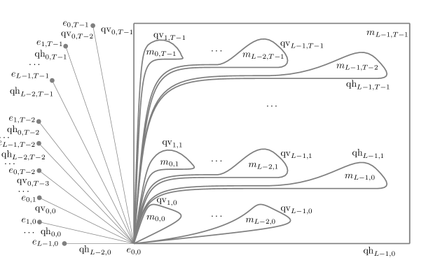
Figure 13: General toric code simplification, step 5. Final lattice.

Hence, the operation $\mathcal{U}_{4}\mathcal{U}_{3}\mathcal{U}_{2}\mathcal{U}_{1}$ diagonalises the Hamiltonian in the sense that (a) logical information does not appear in the Hamiltonian but is encoded in two physical qubits, (b) all independent eigenvalues of stabilisers in the Hamiltonian appear now as eigenvalues of one-body operators. Global topological charge neutrality is ensured by two many-body terms. As explained before, a transformation into two copies of an Ising chain can subsequently be performed.

As regards the efficiency of the procedure, the number of CNOTs to be effected is $\mathcal{O}(LT)$. If operations are parallelised as much as possible, the operation can be performed in $\mathcal{O}(L+T)$ steps.

3 Quantum double models

In this section we apply the ER-inspired scheme described in the Abelian case of the toric code to general quantum double models $\mathrm{D}(G)$ based on non-Abelian groups [1]. While this construction holds exactly, with a more natural structure, in the class of quantum double models $\mathrm{D}(H)$ based on Hopf algebras [4], which contains and generalises the $\mathrm{D}(G)$ models, we settle for a discussion of the group case since the language is bound to be more familiar.

3.1 Hamiltonian, charges

The quantum double model based on a finite group $G$, or $\mathrm{D}(G)$ model, is defined on an 2D lattice $\Lambda$ where quantum degrees of freedom of dimension $\lvert G\rvert$ sit on the edges. Orthonormal bases $\{\lvert g\rangle\}$ are chosen for each oriented edge, labelled by group elements; the bases for the two orientations of any given edge are related by the inversion $g\mapsto g^{-1}$. The Hilbert space of an oriented edge may be identified with the group algebra $\mathbb{C}G$ of complex combinations of group elements.

The Hamiltonian of the $\mathrm{D}(G)$ model is

$$H_{\Lambda}=-\sum_{P}B_{P}-\sum_{V}A_{V}\;,$$ (14)

where the first sum runs over plaquettes of $\Lambda$, the second over vertices of $\Lambda$, and $A_{V}$, $B_{P}$ are mutually commuting projectors with support on the edges adjacent to the vertex and along the boundary of the plaquette, respectively.

Plaquette projectors select configurations where the product of group elements along the plaquette boundaries is the identity element of $G$:

$$B_{P}\,\lvert g_{1},\,g_{2},\,\ldots,\,g_{r}\rangle=\delta_{e}(g_{r}\ldots g_{2}g_{1})\,\lvert g_{1},\,g_{2},\,\ldots,\,g_{r}\rangle\;,$$ (15)

where $g_{1},\,\ldots,\,g_{r}$ are group elements defining a computational basis state of the edges along the plaquette boundary, oriented and ordered along an anticlockwise circuit with arbitrary origin, as illustrated in figure 14. Vertex projectors have the form

$$A_{V}\,\lvert g_{1},\,g_{2},\,\ldots,\,g_{s}\rangle=\frac{1}{\lvert G\rvert}\,\sum_{k\in G}\lvert kg_{1},\,kg_{2},\,\ldots,\,kg_{s}\rangle\;,$$ (16)

where $g_{1},\,\ldots,\,g_{s}$ are group elements defining a computational basis ket in the bonds adjacent to the vertex, oriented towards it, as in figure 14.

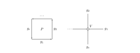
Figure 14: Quantum double Hamiltonian. Conventions for the definition of plaquette and vertex projectors in equations (15) and (16).

Simultaneous $+1$ eigenstates of all $A_{V}$ and $B_{P}$ are ground states, and excited states break the ground state conditions $A_{V}\lvert\psi\rangle=\lvert\psi\rangle$, $B_{P}\lvert\psi\rangle=\lvert\psi\rangle$ at some vertices or plaquettes. We can speak of particle-like excitations living at broken plaquettes and vertices, and it turns out that these particles are characterised by topological charges from an anyon model [20]. Topological charges are properties of regions that cannot be changed by physical operations within the region, and can be determined from measurements on its boundary (think of electric charge, measured by Gauss’s law); more generally, a topological charge label can be assigned to any closed loop independently of whether it is the boundary of a region or not, which is crucial for the study of topologically nontrivial systems, as we will see in the next section.

Topological charges in the quantum double models can be understood algebraically: they are labelled by irreducible representations of Drinfel’d’s quantum double $\mathrm{D}(G)$, a quasitriangular Hopf algebra which can be computed for each group $G$ [21]. More details will be given later; for the moment let us remark that the distribution of topological charge on the lattice may be characterised locally by assigning charge labels to lattice sites, where, following Kitaev, a site is a pair of a plaquette and one of its neighbouring vertices. A charge has thus in general a magnetic part, associated with the plaquette, and an electric part, associated with the vertex; a charge with both nontrivial magnetic and electric parts is called a dyon. The part of Hamiltonian (14) acting on a site assigns energy $-2$ to the trivial charge (the unique charge with trivial electric and magnetic parts), $-1$ to purely magnetic or purely electric charges, and $0$ to dyons.

3.2 The smallest torus

To generalise the treatment of the toric code given in section 2, we first need to understand the topological degrees of freedom of the $\mathrm{D}(G)$ model on the torus, which are not covered by the previous local characterisation of topological charge distributions.

In the toric code, the ground level has fourfold degeneracy; usually this is interpreted as the set of states of two logical qubits associated with the two noncontractible loops on $\mathrm{T}^{2}$ as in the left part of figure 15. The logical Pauli $Z_{\mathrm{hor}}$ and $Z_{\mathrm{vert}}$ measure magnetic quantum numbers $m_{\mathrm{hor}}$, $m_{\mathrm{vert}}$ along the horizontal and vertical loops; this amounts to determining ‘half the topological charge’ for each loop. This defines a basis $\lvert m_{\mathrm{hor}},\,m_{\mathrm{vert}}\rangle_{\mathrm{hv}}$ of eigenstates in the ground level.

Alternatively, one may choose as commuting set of observables the logical Pauli $Z_{\mathrm{hor}}$ along a horizontal loop of the direct lattice, and the logical Pauli $X_{\mathrm{hor}}$ along a horizontal loop of the dual lattice (centre of figure 15). In this case one has a basis $\lvert q_{\mathrm{hor}}\rangle_{\mathrm{h}}$ labelled by the full topological charge label $q_{\mathrm{hor}}=(m_{\mathrm{hor}},\,e_{\mathrm{hor}})$ associated with the horizontal loop, including the eigenvalue $m_{\mathrm{hor}}$ of the magnetic $Z_{\mathrm{hor}}$ operator and the eigenvalue $e_{\mathrm{hor}}$ of the electric $X_{\mathrm{hor}}$ operator.

If we choose the corresponding logical Pauli operators along the vertical loop (figure 15, right), then we have another basis $\lvert q_{\mathrm{vert}}\rangle_{\mathrm{v}}$ labelled by a full topological charge. From the abstract properties of an anyon model [20], we know that the change of basis between $\lvert q_{\mathrm{hor}}\rangle_{\mathrm{h}}$ and $\lvert q_{\mathrm{vert}}\rangle_{\mathrm{v}}$ is the unitary operator known as the topological $S$-matrix:

$$\lvert q_{\mathrm{vert}}\rangle_{\mathrm{v}}=\sum_{q_{\mathrm{hor}}}\lvert q_{\mathrm{hor}}\rangle_{\mathrm{h}}\,S_{q_{\mathrm{hor}},\,q_{\mathrm{vert}}}\;.$$ (17)

This relation encodes a sort of uncertainty principle for topological labels on $\mathrm{T}^{2}$: if we determine the full label along the horizontal loop, the vertical label is ‘maximally spread’, and vice versa. The states of the $\mathrm{hv}$-basis work as sorts of coherent states where a compromise in the measurements of the horizontal and vertical labels is made so as to have mutually commuting observables.

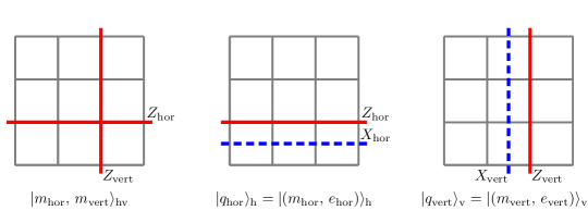
Figure 15: Logical operators in the toric code. Sets of commuting observables yielding complete topological information in the ground level. Left: Two logical Pauli $Z$s measuring ‘half the topological charge’ along each noncontractible loop on $\mathrm{T}^{2}$. Centre: A pair of logical Pauli $Z$ and $X$ measuring the whole topological charge along the horizontal loop. Right: The same for the vertical loop. In each case, the associated bases for the ground level are displayed.

When considering non-Abelian models, we should not expect the $\mathrm{hv}$-basis to survive. Indeed, in an Abelian $\mathrm{D}(G)$ model the number of topological sectors is $\lvert G\rvert^{2}$, a perfect square, and one can successfully construct the $\lvert m_{\mathrm{hor}},\,m_{\mathrm{vert}}\rangle_{\mathrm{hv}}$ states due to the separation of electric and magnetic degrees of freedom. In a non-Abelian $\mathrm{D}(G)$ model one has in general a number of charges different from a perfect square, for instance eight charges in the $\mathrm{D}(\mathrm{S}_{3})$ model.

However, the $\mathrm{h}$-basis and the $\mathrm{v}$-basis can be generalised for non-Abelian models. More than that, their existence stems from the modular nature of the underlying anyon model and is therefore a fundamental property.

As in the Abelian case, a quantum double model on the minimal toric lattice consisting of two edges contains the full basis of the ground level; in contrast with the Abelian case, the Hilbert space of these two qudits is not identical with the ground level, that is, there is room for excitations even in such a small system. Exactly for which excitations is ultimately a representation-theoretical problem.

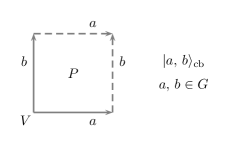
Figure 16: Computational basis for the minimal torus in the $\mathrm{D}(G)$ model.

To wit, let $\lvert a,\,b\rangle_{\mathrm{cb}}$ be the elements of the computational basis for the minimal torus, with $a,\,b\in G$ (figure 16). The action of the unique plaquette and vertex projectors reads

$$B_{P}\,\lvert a,\,b\rangle_{\mathrm{cb}} =\delta(ab,\,ba)\,\lvert a,\,b\rangle_{\mathrm{cb}}\;,$$

$$A_{V}\,\lvert a,\,b\rangle_{\mathrm{cb}} =\frac{1}{\lvert G\rvert}\,\sum_{g\in G}\lvert gag^{-1},\,gbg^{-1}\rangle_{\mathrm{cb}}\;,$$ (18)

Clearly, if $G$ is Abelian these are always the identity operator, so the Hilbert space of the two qudits is identical with the ground level. But for non-Abelian groups, the conditions $B_{P}\,\lvert\psi\rangle=\lvert\psi\rangle$, $A_{V}\,\lvert\psi\rangle=\lvert\psi\rangle$ are nontrivial. We can specify a state by giving two sets of charge information:

• A horizontal charge label $q_{\mathrm{hor}}$ corresponding to one horizontal nontrivial loop, as in the previous discussion.

• A bulk charge label $q_{\mathrm{bulk}}$ corresponding to the charge sitting at the site defined by the unique plaquette and the unique vertex of the minimal square, together with internal degrees of freedom of the bulk charge as dictated by the microscopic model.

Not all pairs $(q_{\mathrm{hor}},\,q_{\mathrm{bulk}})$ are compatible: in particular, some charges never appear in the bulk, while some bulk charges are incompatible with some, but not all, of the loop charge labels. The condition for such a pair to be compatible is that the fusion of the two charges contains the horizontal charge:

$$q_{\mathrm{hor}}\times q_{\mathrm{bulk}}\rightarrow q_{\mathrm{hor}}+\ldots$$ (19)

The reason for this is consistency of the charge measurement along the loop: if the loop is deformed by sweeping the whole bulk of the torus, the same charge label should be measured in the resulting loop, because of periodicity. Since the new loop is equivalent to the concatenation of the original loop and a loop enclosing the bulk charge, condition (19) follows (see figure 17).

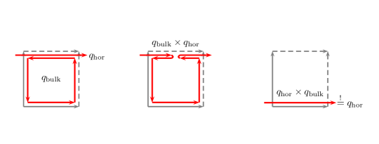
Figure 17: Consistency condition for loop and bulk charges. The loop in the right hand figure is, by periodicity, equivalent to the first horizontal loop, so the charge measured there has to be the same. Since the final loop is obtained by concatenating the original loop and the circuit measuring the bulk charge, the condition $q_{\mathrm{hor}}\times q_{\mathrm{bulk}}\rightarrow q_{\mathrm{hor}}+\ldots$ follows.

The discussion of these phenomena for $\mathrm{D}(G)$ models requires some algebraic machinery and we leave it for appendix A, where we attempt a pedagogical account; the case of the smallest non-Abelian group $\mathrm{S}_{3}$ is considered in appendix B. Here we just list the results:

• Charges in a $\mathrm{D}(G)$ model are labelled by irreducible representations of Drinfel’d’s quantum double algebra $\mathrm{D}(G)$. These are given by pairs $(C,\,\alpha)$, where $C$ are conjugacy classes of $G$, and $\alpha$ are irreducible representations of the centraliser group of $C$; more details appear in appendix A.

• The Hilbert space in the smallest torus consisting of two edges has an orthonormal basis:

  $$\big{\{}\lvert(C,\alpha;k,\,v_{i})_{\mathrm{bulk}};(C^{\prime},\alpha^{\prime})_{\mathrm{hor}}\rangle;\ {}(C,\alpha)\otimes(C^{\prime},\,\alpha^{\prime})\rightarrow(C^{\prime},\,\alpha^{\prime})\oplus\ldots\big{\}}\;,$$ (20)

  where $k,\,v_{i}$ are degrees of freedom determining specific vectors in an irreducible representation space for $(C,\,\alpha)$. The projectors onto definite bulk and horizontal charge labels are given in equation (A) in appendix A.

• From the point of view of the Hamiltonian of the $\mathrm{D}(G)$ model, configurations with vacuum bulk charge $(C_{e},\,1_{+})$ (where the conjugacy class is $C_{e}=\{e\}$, and $1_{+}$ is the trivial representation of $G$) are ground states, with energy $-2$. The energy of states with pure magnetic charges $(C,\,1_{+})$ (where $C\neq C_{e}$, and $1_{+}$ is the trivial representation of the centraliser of $C$) and that of pure electric charges $(C_{e},\alpha)$ (where $\alpha\neq 1_{+}$) in the bulk is $-1$, due to the breakdown of the vertex and plaquette condition, respectively. Finally, the energy of states with a bulk charge $(C,\,\alpha)$ that breaks both the plaquette and vertex conditions ($C\neq C_{e}$, $\alpha\neq 1_{+}$) is $0$.

3.3 Elementary moves

The generalisation of the Abelian P-moves and V-moves to non-Abelian quantum double models was given in the Appendix of the preprint version of [8], in the case of groups; essentially, the CNOT operations of the Abelian case turn into controlled multiplication operators of the type $\lvert g,\,h\rangle\mapsto\lvert g,\,gh\rangle$ and their variants obtained by changes of orientation of the edges for control and target qudits, and these operators are composed to build the elementary moves. For models based on Hopf algebras, the elementary moves, also constructed from controlled multiplications, were defined in [4] and give rise to a MERA for the ground states and the disentangling procedure of this paper in an analogous way; but as already mentioned, we concentrate on the case of groups here. We will not give general expressions, but concentrate on simple examples from which the general procedure is straightforwardly inferred.

A plaquette move or P-move has to be specified more carefully than in the Abelian case, since controlled multiplication operators acting on a target qudit no longer commute with each other. In general, we need specify both a plaquette and one of its edges as a target, or equivalently, one of the vertices along the boundary of the plaquette. A convention necessarily links the specific multiplication operators and the lattice transformation, including the orientation of the edges: ours is defined in figure 18, which we choose to associate with the site $(P_{0},\,V_{0})$.

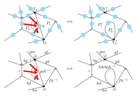
Figure 18: P-moves for a general $\mathrm{D}(G)$ model. Solid arrows stand for controlled left group multiplication operators in the form $\lvert g,\,h\rangle\mapsto\lvert g,\,gh\rangle$; these are to be applied in the order defined by the dotted arrow, assuming the orientation of the edges involved as in the figure. All labels are group elements; therefore we show kets in the computational basis. We give the action of vertex representations of the group (gauge transformations) by showing how elements $h$, $g$ are represented in the vertices $V_{0}$, $V_{1}$ at the boundary of the target edge. After the P-move, the result is clearly a quantum double model in the new lattice that we draw, where the target edge talks twice to the lowermost vertex $V^{\prime}_{0}$ and no longer has contact with the uppermost vertex $V^{\prime}_{1}$. This we call a P-move associated with site $(P_{0},\,V_{0})$.

The vertex moves or V-moves are defined analogously, with the difference that one uses controlled multiplications with a single control and multiple targets, that commute with each other, so one does not need to apply these operations in a certain order. In the models based on Hopf algebras, this commutativity property is lost and one has to take care of the order of operations as well [4] (the property that makes the group case simpler is the cocommutativity of the Hopf structure in group algebras). Our conventions are defined in figure 19, illustrating a V-move which we associate with the site $(V_{0},\,P_{0})$.

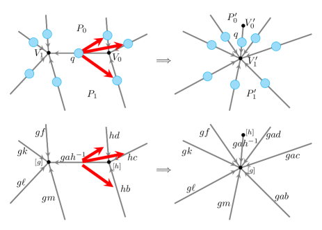
Figure 19: V-moves for a general $\mathrm{D}(G)$ model. Solid arrows, as before, stand for controlled multiplications $\lvert g,\,h\rangle\mapsto\lvert g,\,gh\rangle$; here they need not be applied in any particular order. The V-move in the computational basis, as well as gauge transformations at the affected vertices, are shown in the bottom row. After the move, the control edge is the only one in contact with vertex $V^{\prime}_{0}$, and therefore the only edge feeling the gauge transformation by $h$. The plaquette in which the ‘spike’ is drawn is arbitrary from the point of view of the Hamiltonian; but to be definite we associate this V-move with site $(V_{0},\,P_{0})$.

3.4 Disentangling quantum double models

For the purpose of analysing the quantum double Hamiltonian (14), the only relevant questions are those asked by the vertex and plaquette projectors $A_{v}$, $B_{p}$, whose eigenvalues we may consider a distribution of “binary charges” $e_{v}$, $m_{p}$ taking values in $\{0,\,1\}$. As in the Abelian case, the original Hamiltonian gets transformed into the quantum double Hamiltonian in the deformed lattice, and the “binary charges” get reassigned as depicted in figures 2 and 4. The geometrical moves conserve the number of edges (degrees of freedom), vertices and plaquettes, and the operations on the state are unitaries preserving the energy.

The disentangling procedure for general quantum double Hamiltonians (14) has thus the same graph-theoretical structure as the Abelian cases. The key is that the elementary moves simply redistribute the vertex and plaquette projectors along with the local deformations of the lattice, according to the general rule

$$U_{P(V)}\,H_{\Lambda}\,U_{P(V)}^{\dagger}=H_{\Lambda^{\prime}_{P(V)}}\,\;,$$ (21)

where $\Lambda$ is the original lattice, and $\Lambda^{\prime}_{P(V)}$ are the deformed lattices obtained after the P- and V-moves.

If we work on a topologically nontrivial surface, there appears a difference with the Abelian models. Consider again the case of the torus: eventually the situation simplifies into a lattice where just two “topological” edges go around the two nontrivial cycles, and only one plaquette and one vertex talk (twice each) to them. In the Abelian case the topological edges do not contribute to the dynamics, essentially because the bulk charge in the quantum double model on the small torus consisting of just these two edges, as discussed previously, is always trivial. In a non-Abelian case, the small torus may contain bulk charges, as constrained by condition (19), and these contribute to the energy of the disentangled quantum double model.

More precisely, let us consider the two simple cases analogous to the disentangling of the toric code into mostly sums of one-body operators (figure 6), and the mapping to the double Ising spin chain (figure 7).

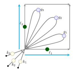
Figure 20: Disentangled quantum double. The lattice for the expression (22) of the Hamiltonian mostly as a sum of one-body terms. In a ket in the computational basis, ‘magnetic’ qudits are in states $\lvert g_{i}\rangle$, ‘electric qudits’ are in states $\lvert k_{j}\rangle$, and topological qudits are in states $\lvert\ell_{1}\rangle$, $\lvert\ell_{2}\rangle$.

In the first case, illustrated in figure 20, the qudits separate into three classes: $r$ ‘magnetic qudits’, whose edges enclose a whole plaquette; $s$ ‘electric’ qudits, whose edges end at a vertex with no other edges attached to it; and two topological qudits. We write a ket in the computational basis as $\lvert g_{1},\,\ldots,\,g_{r};\,k_{1},\,\ldots,k_{s};\,\ell_{1},\,\ell_{2}\rangle$ according to the orientation conventions of figure 20 (where $r=s=3$), where the $\{g_{i}\}$, $\{k_{j}\}$ and $\ell_{1},\,\ell_{2}$ correspond to the magnetic, electric, and topological qudits, respectively. The Hamiltonian reads

$$H=-\,\sum_{i=1}^{r}B_{i}-\,B_{0}-\,\sum_{j=1}^{s}A_{j}-\,A_{0}\;,$$ (22)

where the action of the different operators in the computational basis is

$$B_{i}\, \lvert g_{1},\,\ldots,\,g_{r};\,k_{1},\,\ldots,k_{s};\,\ell_{1},\,\ell_{2}\rangle$$

$$=\delta_{e}(g_{i})\,\lvert g_{1},\,\ldots,\,g_{r};\,k_{1},\,\ldots,k_{s};\,\ell_{1},\,\ell_{2}\rangle\;,$$

$$B_{0}\, \lvert g_{1},\,\ldots,\,g_{r};\,k_{1},\,\ldots,k_{s};\,\ell_{1},\,\ell_{2}\rangle$$

$$=\delta_{e}(g_{1}^{-1}\ldots g_{r}^{-1}\ell_{2}^{-1}\ell_{1}^{-1}\ell_{2}\ell_{1})\,\lvert g_{1},\,\ldots,\,g_{r};\,k_{1},\,\ldots,k_{s};\,\ell_{1},\,\ell_{2}\rangle\;,$$

$$A_{j}\, \lvert g_{1},\,\ldots,\,g_{r};\,k_{1},\,\ldots,k_{s};\,\ell_{1},\,\ell_{2}\rangle$$

$$=\frac{1}{\lvert G\rvert}\,\sum_{n\in G}\lvert g_{1},\,\ldots,\,g_{r};\,k_{1},\,\ldots,k_{j}n^{-1},\,\ldots,\,k_{s};\,\ell_{1},\,\ell_{2}\rangle\;,$$

$$A_{0}\, \lvert g_{1},\,\ldots,\,g_{r};\,k_{1},\,\ldots,k_{s};\,\ell_{1},\,\ell_{2}\rangle$$

$$=\frac{1}{\lvert G\rvert}\,\sum_{n\in G}\lvert ng_{1}n^{-1},\,\ldots,\,ng_{r}n^{-1};\,nk_{1},\,\ldots,nk_{s};\,n\ell_{1}n^{-1},\,n\ell_{2}n^{-1}\rangle\;.$$ (23)

Each $A_{i}$, $B_{j}$ is thus a one-body operator, and the terms $A_{0}$ and $B_{0}$ couple all qudits (except for the electric qubits in the case of $B_{0}$). This generalises Hamiltonian (2.2) for the toric code on the same lattice. Note that the precise location of the spikes is immaterial.

Figure 21: Classical chains for quantum doubles. The lattice for the expression (24) of the Hamiltonian mostly as a sum of two-body terms. The notation is as in figure 20.

In figure 21 we give our conventions for the lattice generalising the double-Ising-chain construction for the toric code. The Hamiltonian is now

$$H=-\,B_{1}-\,\sum_{i=1}^{r-1}B_{i,\,i+1}-\,B_{r,\,0}-\,A_{1}-\,\sum_{j=1}^{s-1}A_{j,\,j+1}-\,A_{s,\,0}\;,$$ (24)

where the different terms are given by

$$B_{1}\, \lvert g_{1},\,\ldots,\,g_{r};\,k_{1},\,\ldots,k_{s};\,\ell_{1},\,\ell_{2}\rangle$$

$$=\delta_{e}(g_{1})\,\lvert g_{1},\,\ldots,\,g_{r};\,k_{1},\,\ldots,k_{s};\,\ell_{1},\,\ell_{2}\rangle\;,$$

$$B_{i,\,i+1}\, \lvert g_{1},\,\ldots,\,g_{r};\,k_{1},\,\ldots,k_{s};\,\ell_{1},\,\ell_{2}\rangle$$

$$=\delta_{e}(g_{i}g_{i+1}^{-1})\,\lvert g_{1},\,\ldots,\,g_{r};\,k_{1},\,\ldots,k_{s};\,\ell_{1},\,\ell_{2}\rangle\;,$$

$$B_{r,\,0}\, \lvert g_{1},\,\ldots,\,g_{r};\,k_{1},\,\ldots,k_{s};\,\ell_{1},\,\ell_{2}\rangle$$

$$=\delta_{e}(g_{r}^{-1}\ell_{2}^{-1}\ell_{1}^{-1}\ell_{2}\ell_{1})\,\lvert g_{1},\,\ldots,\,g_{r};\,k_{1},\,\ldots,k_{s};\,\ell_{1},\,\ell_{2}\rangle\;,$$

$$A_{1}\, \lvert g_{1},\,\ldots,\,g_{r};\,k_{1},\,\ldots,k_{s};\,\ell_{1},\,\ell_{2}\rangle$$

$$=\frac{1}{\lvert G\rvert}\,\sum_{n\in G}\lvert g_{1},\,\ldots,\,g_{r};\,k_{1}n^{-1},\,k_{2},\,\ldots,k_{j},\,\ldots,\,k_{s};\,\ell_{1},\,\ell_{2}\rangle\;,$$

$$A_{j,\,j+1}\, \lvert g_{1},\,\ldots,\,g_{r};\,k_{1},\,\ldots,k_{s};\,\ell_{1},\,\ell_{2}\rangle$$

$$=\frac{1}{\lvert G\rvert}\,\sum_{n\in G}\lvert g_{1},\,\ldots,\,g_{r};\,k_{1},\,\ldots,nk_{j},\,k_{j+1}n^{-1},\,\ldots,\,k_{s};\,\ell_{1},\,\ell_{2}\rangle\;,$$

$$A_{s,\,0}\, \lvert g_{1},\,\ldots,\,g_{r};\,k_{1},\,\ldots,k_{s};\,\ell_{1},\,\ell_{2}\rangle$$

$$=\frac{1}{\lvert G\rvert}\,\sum_{n\in G}\lvert ng_{1}n^{-1},\,\ldots,\,ng_{r}n^{-1};\,k_{1},\,\ldots,,\,k_{s-1},\,nk_{s};\,n\ell_{1}n^{-1},\,n\ell_{2}n^{-1}\rangle\;.$$ (25)

Terms $B_{1}$, $A_{1}$ are one-body, and terms $B_{i,\,i+1}$ and $A_{j,j+1}$ are two-body (and define spin models which are essentially classical since all these terms commute); the projector $B_{r,\,0}$ couples one of the magnetic qudits with the topological edges (that this is not a many-body operator is one of the simplifications with respect to the general Hopf algebraic case); and $A_{s,\,0}$ couples the topological qudits with one of the electric edges and all of the magnetic edges. This generalises the double-Ising-chain mapping, with the terms $B_{r,\,0}$, $A_{s,\,0}$ representing the toric boundary conditions. The topological degeneracy is recovered easily: because of the one-body projectors $B_{1}$, $A_{1}$ breaking the degeneracy of the two-body chains, the ground states of (24) feature product states in all the magnetic and electric qudits; and the remaining degrees of freedom are just the topological qudits, that is, the edges of the minimal torus studied in section 3.2, with the Hamiltonian $-B_{P}-A_{V}$ defined by the operators in (3.2). Explicitly, the ground states of (24) are

$$\frac{1}{\lvert G\rvert^{(s+1)/2}}\,\sum_{n_{1},\,\ldots,n_{s},\,n_{0}\in G}\lvert e,\,\ldots,\,e;\,n_{1},\,\ldots,n_{s};\,n_{0}\ell_{1}n_{0}^{-1},\,n_{0}\ell_{2}n_{0}^{-1}\rangle$$ (26)

where $\ell_{1}$, $\ell_{2}$ are mutually commuting elements of $G$.

3.5 The algebraic meaning

The significance of the elementary moves goes beyond the mere fact that they intertwine the quantum double Hamiltonians in the two lattices. More fundamentally, accompanying the geometrical evolution there is a topological charge redistribution more detailed than just the reshuffling of binary magnetic and electric labels.

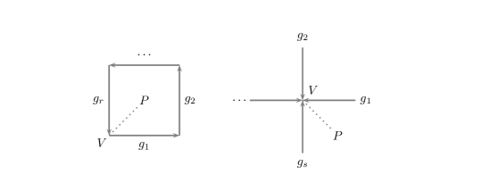
Figure 22: The quantum double algebra. Conventions for the definition of plaquette and vertex representations (27), (28).

Consider again the problem of the local distribution of topological charges in an arbitrary state of a quantum double model. Instead of characterising this distribution of charges by a collection of charge labels at different sites (recall that a site is a pair of neighbouring plaquette and vertex, and that charge labels in general do not split cleanly into a magnetic and electric part), we can choose to endow the system with an algebra of local operators generalising projectors (15) and (16). Plaquette operators are representations of the algebra of functions $f$ from $\mathbb{C}G$ to the complex numbers,

$$B_{P,V}(f)\,\lvert g_{1},\,g_{2},\,\ldots,\,g_{r}\rangle=f(g_{r}\ldots g_{2}g_{1})\,\lvert g_{1},\,g_{2},\,\ldots,\,g_{r}\rangle\;,$$ (27)

and vertex operators are representations of $\mathbb{C}G$, defined by

$$A_{V,P}(k)\,\lvert g_{1},\,g_{2},\,\ldots,\,g_{s}\rangle=A_{V}(k)\,\lvert g_{1},\,g_{2},\,\ldots,\,g_{s}\rangle=\lvert kg_{1},\,kg_{2},\,\ldots,\,kg_{s}\rangle\;,$$ (28)

in the conventions of figure 22. It can be shown that the $B_{P,V}(f)$ and $A_{V,P}(k)$ operators acting on a site define a reducible representation of $\mathrm{D}(G)$, decomposing into the different charge sectors for that site. Hence, we can simply say that the charge distribution is determined locally by the reaction of the lattice state to operators (27) and (28), for the different plaquettes and vertices. This has the advantage that we can work with plaquettes and vertices separately, without the complications due to the intricate nature of dyonic charges. Note that vertex operators (28) do not depend on the plaquette; this property is lost in the more general Hopf algebraic setting of [4].

The deepest property of the elementary moves is that they are intertwiners for representations $A_{V,P}(g)$ and $B_{P,V}(f)$ along the flow of lattice deformations they define. (Ultimately, these moves realise morphisms in a category of representations.) The most complete approach to this deep property would entail a full study of the transformations of Kitaev’s ribbon operators [1], the building blocks of the representations $A_{V}(g)$ and $B_{P}(f)$, under elementary moves, but for this paper we will just cover the transformation of the latter, and do so using figures.

The general form of the intertwining property is

$$U_{s_{0}}\,A_{s}(g)=A_{s^{\prime}}(g)\,U_{s_{0}}\;,\qquad U_{s_{0}}\,B_{s}(f)=B_{s^{\prime}}(f)\,U_{s_{0}}\;,$$ (29)

where the move is either a plaquette or a vertex move associated with site $s_{0}$, and $s^{\prime}$ is the image of $s$ after the lattice deformation. This obviously implies the intertwining property for the Hamiltonian, but is much more general. The transformation of the sites is subtle, though, and the notion of site as strict neighbouring pair has to be relaxed. Let us consider the examples that we already used to define the general moves.

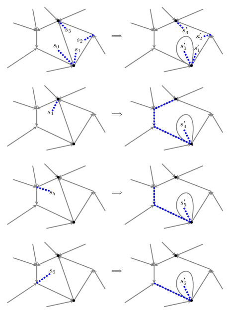
Figure 23: Transformation of sites upon P-moves. The $P$-move of figure 18 is associated with site $s_{0}$. Sites having the plaquette $P_{0}$ in common with $s_{0}$ have a subtle transformation involving a path along the boundary of this plaquette.

Any elementary move deforms one edge, which talks to two plaquettes $P_{0},\,P_{1}$ and two vertices $V_{0},\,V_{1}$. In our convention, moves are associated with one site, say $s_{0}=(P_{0},\,V_{0})$. Consider the P-move studied in figure 18, and the transformation of representations $A_{V,\,P}(g)$ and $B_{P,V}(f)$ encoded in the geometric transformation of sites. In general, sites transform as $s=(P,\,V)\mapsto s^{\prime}=(P^{\prime},\,V^{\prime})$ according to the images of $P$ and $V$ under the deformation of the lattice (first row of figure 23). However, sites of the form $s=(P_{0},V)$ with $V\neq V_{0}$ have a more subtle transformation, as shown in the last three rows of figure 23. In those cases, $s^{\prime}=(P^{\prime}_{0}{}^{V^{\prime}V^{\prime}_{0}},V^{\prime}_{0})$, where $P^{\prime}_{0}{}^{V^{\prime}V^{\prime}_{0}}$ is the plaquette $P^{\prime}_{0}$ conjugated by the path from $V^{\prime}$ to $V^{\prime}_{0}$ along the boundary of $P_{0}$. Operationally, this means that representations $A_{V}$ get transformed into $A_{V^{\prime}}$, and $B_{P}$ gets transformed into an operator whose argument is the conjugation of the group element along the boundary edge of $P^{\prime}_{0}$ by the product of group elements along the path $V^{\prime}V^{\prime}_{0}$ (this conjugation is invisible for the operators entering the Hamiltonian).

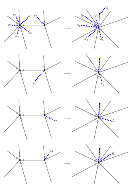
Figure 24: Transformation of sites under V-moves. The move in figure 19 is associated with site $s_{0}$. Sites having the vertex in common with $s_{0}$ have again a nontrivial transformation.

V-moves can be analysed in much the same way. Consider the move in figure 19, associated with site $s_{0}=(P_{0},\,V_{0})$. Sites transform again as $s=(P,\,V)\mapsto s^{\prime}=(P^{\prime},\,V^{\prime})$ except for those having $V_{0}$ as a vertex and $P\neq P_{0}$ (note that $s_{0}$ itself transforms into $(P^{\prime}_{0},V^{\prime}_{0})$). We have $s=(P,\,V_{0})\mapsto(P^{\prime}{}^{V^{\prime}_{0}V^{\prime}_{1}},V^{\prime}_{0})$, that is, the plaquette is conjugated by a path from $V^{\prime}_{0}$ to $V^{\prime}_{1}$ (see figure 24).

4 Discussion

In summary, we have extended the entanglement renormalisation approach for ground states of topological lattice systems to a unitary quantum circuit disentangling procedure that diagonalises the Hamiltonian. We give this construction for Kitaev’s quantum double models based on groups, on the understanding that the construction generalises directly to more general quantum double models based on Hopf $C^{\ast}$-algebras. The extension of the Abelian construction to the non-Abelian case is informed by the understanding of the structure of the Hilbert space and energy levels in the toric topology, and we give an account of this with details and a specific example to be found in the appendices.

While this ER picture extended to the full spectrum of the quantum doubles is geometrically pleasant, it is probably not a practical way to construct the relevant codes from a small instance by adding degrees of freedom, since it requires very nonlocal operations.

Note that the double Ising chain lurking behind the toric code has been exposed by different authors. In particular, a duality mapping was given in [22] showing that the partition function of the toric code is identical to that of two noninteracting Ising chains. The construction presented here is graphic and explicit, and lends itself to generalisation for non-Abelian quantum double models. It also uncovers an intriguing geometrical picture of renormalisation, proceeding through deformations simplifying the original lattice, that can probably be extended to general string-net models building upon the work in [9].

On the other hand, what we achieve in the end is (up to boundary conditions) the diagonalisation of a Hamiltonian consisting of mutually commuting projectors. The approach of Ref. [17] is a general method for diagonalising strongly correlated Hamiltonians in terms of a quantum circuit, and the present work can be regarded as an illustration thereof (the tensor network behind this construction being a unitary quantum circuit obtained from unitarisation of the ER scheme of [8]).

As remarked in the introduction, a lattice is essentially a discretisation of the metric in a continuum theory. One of the notable points of this construction is that the flow of the quantum circuit is universal for all the quantum double models, being encoded in the simplifying moves acting on the lattice structure: whether this points to a meaningful procedure in the continuum limit is a suggestive question.

Work using related geometrical ideas, leading to numerical methods for the $\mathbb{Z}_{2}$ gauge theory, was reported in [18]. Similar ideas are being used by R. König, F. Verstraete, and collaborators, working towards a more general renormalisation scheme for lattice systems, to be found in [23].

Acknowledgements

I thank Guifré Vidal, Gavin Brennen, Oliver Buerschaper and Sofyan Iblisdir for key discussions on quantum double models, Robert König and Frank Verstraete for generous communication about their work, and the Kavli Institute for Theoretical Physics for hospitality during the research programme Disentangling quantum many-body systems: Computational and conceptual approaches. This research was supported in part by the National Science Foundation under Grant No. NSF PHY05-51164.

Appendix A Topological charges in $\mathrm{D}(G)$ models

In a $\mathrm{D}(G)$ model, topological charges are given in terms of the group structure and its representation theory (in the recent paper [24], it was shown that not all such charges are physically distinguishable; however, we will not be concerned with these issues here). Charge labels are pairs $(C,\,\alpha)$, where:

• $C$ runs over conjugacy classes of the group, that is, orbits of group elements under the adjoint action $t\mapsto gtg^{-1}$.

• $\alpha$ runs over irreducible representations (irreps) of the centraliser group $N_{C}$ of the conjugacy class $C$.

The centraliser $N_{C}$ is constructed as follows: given $c\in C$, its centraliser $N_{c}$ is the subgroup of $G$ consisting of all the elements of $G$ commuting with $c$,

$$N_{c}=\{n\in G;\;ncn^{-1}=c\}\;.$$ (30)

It is immediately checked that

$$n\in N_{c}\quad\Rightarrow\quad gng^{-1}\in N_{gcg^{-1}}\;,$$ (31)

so the centralisers of elements of the same conjugacy class are conjugate (and hence, isomorphic) to each other, justifying the definition of the abstract $N_{C}$. The size of this group is $\lvert N_{C}\rvert=\lvert G\rvert/\lvert C\rvert$.

Pairs $(C,\,\alpha)$ correspond to irreducible representations of the quantum double $\mathrm{D}(G)$; for the purposes of this work, it suffices to present $\mathrm{D}(G)$ as the tensor product $\mathbb{C}^{G}\otimes\mathbb{C}G$ of the space of complex functions on the group and the space of complex linear combinations of group elements, or group algebra. This vector space is spanned by elements $P_{h}g\equiv\delta_{h}\otimes g$, where $g,\,h\in G$, and $\delta_{h}:k\mapsto\delta_{h,\,k}$ are Kronecker delta functions. The algebra structure in $\mathrm{D}(G)$ is given by the multiplication

$$P_{h}g\cdot P_{k}\ell=\delta_{h}(gkg^{-1})\,P_{h}g\ell\;.$$ (32)

An irreducible representation $(C,\,\alpha)$ of $\mathrm{D}(G)$ realises elements $P_{h}g$ as endomorphisms of a linear representation space $V^{(C,\,\alpha)}$; this can be identified with $\mathbb{C}C\otimes V^{\alpha}$, where $V^{\alpha}$ is the representation space for group representation $\alpha$. A basis of $V^{(C,\,\alpha)}$ is given by $\{\lvert k;\,v_{i}\rangle\}$, with $k\in C$ and $\{\lvert v_{i}\rangle\}$ a basis of $V^{\alpha}$, such that

$$D^{\alpha}(n)\,\lvert v_{i}\rangle=\sum_{j}\lvert v_{j}\rangle\,D^{\alpha}_{ji}(n)\;,\quad n\in N_{C}\;.$$ (33)

The matrix form of $(C,\,\alpha)$ reads [25, 26]

$$D^{(C,\,\alpha)}(P_{h}g)\,\lvert k,\,v_{i}\rangle=\delta_{h}(gkg^{-1})\,\sum_{j}\lvert gkg^{-1},\,v_{j}\rangle\,D^{\alpha}_{ji}(g\rvert_{N_{k_{0}}})\;,$$ (34)

or, in other words,

$$D^{(C,\,\alpha)}_{\ell j,\,ki}(P_{h}g)=\delta_{\ell}(gkg^{-1})\,\delta_{h}(gkg^{-1})\,D^{\alpha}_{ji}(g\rvert_{N_{k_{0}}})\;.$$ (35)

Here $k_{0}$ is an arbitrarily chosen reference element in conjugacy class $C$, and $\alpha$ is chosen as a representation of the normaliser $N_{k_{0}}$. The notation $g\rvert_{N_{k_{0}}}$ means a projection of $g\in G$ onto $N_{k_{0}}$, defined as follows: given the reference $k_{0}\in C$, define a system of group elements $x_{k_{0}}^{k}\in G$, one for each $k\in C$, such that $x_{k_{0}}^{k}k_{0}(x_{k_{0}}^{k})^{-1}=k$, and in particular $x_{k_{0}}^{k_{0}}=e$. It can be checked that $x_{k_{0}}^{k}N_{k_{0}}$ are mutually disjoint cosets whose union is $G$. Now the adjoint action of $g$ maps $k$ to $gkg^{-1}$, and from this follows that $g\rvert_{N_{k_{0}}}\equiv(x_{k_{0}}^{gkg^{-1}})^{-1}gx_{k_{0}}^{k}$ is an element of $N_{k_{0}}$, which is what appears in (34) and (35). Different choices of $k_{0}$ and $\{x_{k_{0}}^{k}\}$ give rise to equivalent representations.

The left regular representation, that is, the representation of $\mathrm{D}(G)$ on $\mathrm{D}(G)$ defined by left multiplication

$$a\mapsto L(a)\;,\quad L(a):b\mapsto ab\;,$$ (36)

is reducible and contains each one of the irreps $(C,\,\alpha)$ of $\mathrm{D}(G)$ with a multiplicity equal to its dimension $\lvert C\rvert\lvert\alpha\rvert$, just as for finite groups:

$$\mathrm{D}(G)\approx\bigoplus_{(C,\,\alpha)}\bigoplus_{a=1}^{\lvert C\rvert\lvert\alpha\rvert}V^{(C,\,\alpha)}_{a}\;.$$ (37)

Explicitly, the following elements of $\mathrm{D}(G)$:

$$[(C,\,\alpha)\,k,\,\ell;\,i,\,s]=\sqrt{\frac{\lvert C\rvert\lvert\alpha\rvert}{\lvert G\rvert}}\,P_{k}\,\sum_{n\in N_{k}}D^{\alpha}_{si}\big{(}(x_{k_{0}}^{k})^{-1}n^{-1}x_{k_{0}}^{k}\big{)}\,n\,x_{k_{0}}^{k}\,(x_{k_{0}}^{\ell})^{-1}\,,$$ (38)

where $k,\,m\in C$, are a basis of the quantum double algebra satisfying

$$P_{h}g \,\cdot\,[(C,\,\alpha)\,k,\,\ell;\,i,\,s]$$

$$=\delta_{h}(gkg^{-1})\,\sum_{j}[(C,\,\alpha)\,gkg^{-1},\,\ell;\,j,\,s]\;D^{\alpha}_{ji}\big{(}(x_{k_{0}}^{gkg^{-1}})^{-1}gx_{k_{0}}^{k}\big{)}\,,$$ (39)

and hence, they realise decomposition (37) if we identify index $a$ with the pair $(\ell,\,s)$.

Projection onto the different $(C,\,\alpha)$ sectors in $\mathrm{D}(G)$ is achieved by multiplication with the following central algebra elements:

$$\mathcal{Q}^{(C,\,\alpha)}=\frac{\lvert C\rvert\lvert\alpha\rvert}{\lvert G\rvert}\,\sum_{k\in C}\sum_{n\in N_{k}}\chi^{\alpha}\big{(}(x_{k_{0}}^{k})^{-1}n^{-1}x_{k_{0}}^{k}\big{)}\,P_{k}\,n\;,$$ (40)

where $\chi^{\alpha}$ is the character of representation $\alpha$. It can be checked that they form a decomposition of the unit into a sum of projectors:

$$\mathcal{Q}^{(C,\,\alpha)}\cdot\mathcal{Q}^{(C^{\prime},\,\alpha^{\prime})}=\delta^{(C,\,\alpha),\,(C^{\prime},\,\alpha^{\prime})}\,\mathcal{Q}^{(C,\,\alpha)}\;,\quad\sum_{(C,\,\alpha)}\mathcal{Q}^{(C,\,\alpha)}=1_{\mathrm{D}(G)}=\sum_{h}P_{h}e\;.$$ (41)

Upon multiplication, they project onto the irrep blocks $\bigoplus_{a}V^{(C,\,\alpha)}_{a}$ of decomposition (37):

$$\mathcal{Q}^{(C,\,\alpha)}\,\cdot\,[(C^{\prime},\,\alpha^{\prime})\,k,\,\ell;\,i,\,s]=\delta^{(C,\,\alpha),\,(C^{\prime},\,\alpha^{\prime})}\,[(C^{\prime},\,\alpha^{\prime})\,k,\,\ell;\,i,\,s]\;.$$ (42)

The key algebraic structure defined on the $\mathrm{D}(G)$ lattice models is the algebra of ribbon operators [1] (see also [27] for a very readable introduction). Without going into the details of the definition, these operators are assembled from one-edge operators $L_{\pm}(g)$ representing $G$ (or, more generally, the group algebra $\mathbb{C}G$), and $T_{\pm}(f)$ representing the dual algebra $\mathbb{C}^{G}$ of complex functions on $G$:

$$L_{+}(g)\,a=ga\,,\quad L_{-}(g)\,a=ag^{-1}\,,\quad T_{+}(f)\,a=f(a)\,a\,,\quad T_{-}(f)\,a=f(a^{-1})\,a\;.$$ (43)

The $L_{\pm}$ are just the left and right regular representations of $\mathbb{C}G$, while the $T_{\pm}$ are equivalent to the left and right regular representations of $\mathbb{C}^{G}$ (through the map $g\mapsto\sqrt{\lvert G\rvert}\,\delta_{g^{-1}}$, which is an electric-magnetic duality [5]).

By forming combinations of these elementary operations using the properties of $\mathbb{C}G$ and $\mathbb{C}^{G}$ as Hopf algebras, one can build representations of $\mathrm{D}(G)$ and its dual. In particular, one can define projectors to ‘measure the topological charge’ associated with geometrical closed ribbons by representing the elements $\mathcal{Q}^{(C,\,\alpha)}\in\mathrm{D}(G)$.

Coming back to our smallest torus, we define topological labels for a horizontal loop, a vertical loop, and the bulk site, using the following representations of $\mathrm{D}(G)$:

$$F_{\mathrm{hor}}(P_{h}g)\,\lvert a,\,b\rangle_{\mathrm{cb}} =\delta_{h}(gag^{-1})\,\lvert gag^{-1},\,gb\rangle_{\mathrm{cb}}\;,$$

$$F_{\mathrm{vert}}(P_{h}g)\,\lvert a,\,b\rangle_{\mathrm{cb}} =\delta_{h^{-1}}(gbg^{-1})\,\lvert ga,\,gbg^{-1}\rangle_{\mathrm{cb}}\;,$$

$$F_{\mathrm{bulk}}(P_{h}g)\,\lvert a,\,b\rangle_{\mathrm{cb}} =\delta_{h}(gb^{-1}a^{-1}bag^{-1})\,\lvert gag^{-1},\,gbg^{-1}\rangle_{\mathrm{cb}}\;.$$ (44)

From these representations, the projectors onto definite topological sectors are

$$F_{\mathrm{hor}}\big{(}\mathcal{Q}^{(C,\,\alpha)}\big{)}\,\lvert a,\,b\rangle_{\mathrm{cb}} =\frac{\lvert C\rvert\lvert\alpha\rvert}{\lvert G\rvert}\,\sum_{k\in C}\delta_{k}(a)\,\sum_{n\in N_{k}}\chi^{\alpha}\big{(}(x_{k_{0}}^{k})^{-1}n^{-1}x_{k_{0}}^{k}\big{)}\,\lvert a,\,nb\rangle_{\mathrm{cb}}\;,$$

$$F_{\mathrm{vert}}\big{(}\mathcal{Q}^{(C,\,\alpha)}\big{)}\,\lvert a,\,b\rangle_{\mathrm{cb}} =\frac{\lvert C\rvert\lvert\alpha\rvert}{\lvert G\rvert}\,\sum_{k\in C}\delta_{k^{-1}}(b)\,\sum_{n\in N_{k}}\chi^{\alpha}\big{(}(x_{k_{0}}^{k})^{-1}n^{-1}x_{k_{0}}^{k}\big{)}\,\lvert na,\,b\rangle_{\mathrm{cb}}\;,$$

$$F_{\mathrm{bulk}}\big{(}\mathcal{Q}^{(C,\,\alpha)}\big{)}\,\lvert a,\,b\rangle_{\mathrm{cb}}$$

$$=\frac{\lvert C\rvert\lvert\alpha\rvert}{\lvert G\rvert}\,\sum_{k\in C} \delta_{k}(b^{-1}a^{-1}ba)\,\sum_{n\in N_{k}}\chi^{\alpha}\big{(}(x_{k_{0}}^{k})^{-1}n^{-1}x_{k_{0}}^{k}\big{)}\,\lvert nan^{-1},\,nbn^{-1}\rangle_{\mathrm{cb}}\;.$$ (45)

Projectors $F_{\mathrm{bulk}}\big{(}\mathcal{Q}^{(C,\,\alpha)}\big{)}$ commute both with horizontal and with vertical projectors in (A). This justifies a labelling of states in the small torus Hilbert space by a bulk charge and a loop charge (horizontal or vertical). The bulk charge is relevant for the energy, since the Hamiltonian penalises the departure from trivial charge in the bulk; loop labels, on the other hand, do not play a rôle for the Hamiltonian.

The ground level of the quantum double Hamiltonian is the $+1$ eigenspace of the projector

$$F_{\mathrm{bulk}}\big{(}\mathcal{Q}^{(C_{e},\,1_{+})}\big{)}\,\lvert a,\,b\rangle_{\mathrm{cb}}=\frac{1}{\lvert G\rvert}\,\sum_{n\in G}\delta_{e}(b^{-1}a^{-1}ba)\,\lvert nan^{-1},\,nbn^{-1}\rangle_{\mathrm{cb}}\;.$$ (46)

It is easy to check that the dimension of this vacuum subspace equals the number of topological charge labels. We can give an orthonormal basis labelled by a charge label in the horizontal loop, i. e., the $\mathrm{h}$-basis, as

$$\lvert(C,\,\alpha)\rangle_{\mathrm{h}}=\frac{1}{\sqrt{\lvert G\rvert}}\,\sum_{k\in C}\sum_{n\in N_{k}}\chi^{\alpha}\big{(}(x_{k_{0}}^{k})^{-1}n^{-1}x_{k_{0}}^{k}\big{)}\,\lvert k,\,n\rangle_{\mathrm{cb}}\;,$$ (47)

or the alternative $\mathrm{v}$-basis labelled by vertical charges,

$$\lvert(C,\,\alpha)\rangle_{\mathrm{v}}=\frac{1}{\sqrt{\lvert G\rvert}}\,\sum_{k\in C}\sum_{n\in N_{k}}\chi^{\alpha}\big{(}(x_{k_{0}}^{k})^{-1}n^{-1}x_{k_{0}}^{k}\big{)}\,\lvert n,\,k^{-1}\rangle_{\mathrm{cb}}\;.$$ (48)

The overlap of basis states of (47) and (48) gives the topological $S$-matrix of the theory:

$$S_{(C^{\prime},\,\alpha^{\prime}),\,(C,\,\alpha)}={}_{\mathrm{v}}\langle(C^{\prime},\,\alpha^{\prime})|(C,\,\alpha)\rangle_{\mathrm{h}}$$

$$=\frac{1}{\lvert G\rvert}\,\sum_{k\in C}\sum_{\ell\in C^{\prime}\cap N_{k}}\chi^{\alpha^{\prime}}\big{(}(x_{\ell_{0}}^{\ell})^{-1}\,k\,x_{\ell_{0}}^{\ell}\big{)}\,\chi^{\alpha}\big{(}(x_{k_{0}}^{k})^{-1}\,\ell\,x_{k_{0}}^{k}\big{)}\;,$$ (49)

where $k_{0},\,\ell_{0}$ are the reference elements of conjugacy classes $C$, $C^{\prime}$, respectively.

For the whole Hilbert space of the small torus one may expect to find a basis labelled by a loop charge, say the horizontal label, and a bulk charge (plus possibly internal degrees of freedom for the latter). This is a good strategy, but in general not all such charge pairs are compatible. For Abelian $G$ only the trivial charge may appear in the bulk. For non-Abelian models, some charges can never appear in the bulk, and additionally some bulk charges are excluded depending on the loop charge label. Exactly which charges may appear in the bulk is a property of the anyon model and ultimately a representation-theoretical problem. As argued in the text, the compatible pairs of bulk charge and loop charge are those that can fuse into the loop charge. If the group $G$ is Abelian, the representation theory of $\mathrm{D}(G)$ is Abelian and charges are only invariant if they fuse with the vacuum charge $(C_{e},\,1_{+})$; this singles out the vacuum label as the only possible bulk charge. For non-Abelian models, the allowed pairs must be computed from the fusion rules. We give the full details for $G=\mathrm{S}_{3}$ in appendix B.

A comment on the notion of charge in the bulk is in order. The projectors $F_{\mathrm{bulk}}(\mathcal{Q}^{(C,\,\alpha)})$ probe the topological charge in a contractible region, namely the square defined by the edges (square $aba^{-1}b^{-1}$ in figure 25); this happens to cover the whole area of the torus but cannot see topological quantities, because it does not include the boundary conditions. If one measures nontrivial topological charge on the bulk, it is exactly compensated by an opposite charge sitting at the boundary, and measured along the opposite circuit ($bab^{-1}a^{-1}$ in the notation of figure 25). All in all, the total charge on the whole torus corresponds to a measurement along a circuit equivalent to that in the right part of figure 25, that is, a loop always homotopic to a point, which always yields the trivial charge.

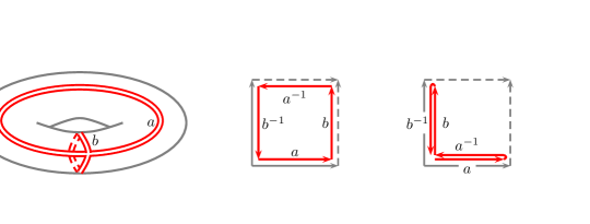
Figure 25: Definition of bulk charges on the smallest torus. Cutting a torus into a square defines a contractible region, with a boundary along the circuit $aba^{-1}b^{-1}$. The charge measured in this region is what we call bulk charge. The question of the total charge on the surface of the torus corresponds to the circuit $aa^{-1}bb^{-1}$, yielding always the trivial charge.

The way in which bulk charge appears in the non-Abelian $\mathrm{D}(G)$ models is one aspect of Kitaev’s construction which differs from a theory of gauge fields. In a discrete gauge theory, edge variables are gauge variant; therefore, toric boundary conditions only fix the periodicity of the edge variables up to a gauge transformation defined on the boundary of the bulk, which in turn is related to the bulk charge (in, for instance, a $U(1)$ gauge theory, single-valuedness of the gauge transformation imposes Dirac’s quantisation condition, which constrains the value of the bulk magnetic flux). In Kitaev’s lattice models, however, edge variables correspond to physical states of physical qudits, which are strictly periodic on the torus.

Appendix B $\mathrm{S}_{3}$ and the $\mathrm{D}(\mathrm{S}_{3})$ model

In this appendix we illustrate the general formalism for the smallest non-Abelian group and the associated quantum double model.

Let $G=\mathrm{S}_{3}$ be the group of permutations of three objects. It has six elements, organised into three conjugacy classes: the unit $e$; the transpositions $t_{0}=(12)$, $t_{1}=(23)$, $t_{2}=(31)$; and the $3$-cycles $c_{+}=(123)$, $c_{-}=(132)$.

The topological sectors of the $\mathrm{D}(\mathrm{S}_{3})$ model, that is, the irreducible representations of the quantum double algebra $\mathrm{D}(\mathrm{S}_{3})$, are labelled by pairs $(C,\,\alpha)$, where $C$ is one of the conjugacy classes $C_{e}=\{e\}$, $C_{t}=\{t_{0},\,t_{1},\,t_{2}\}$, and $C_{c}=\{c_{+},\,c_{-}\}$, and $\alpha$ is an irrep of the centraliser $N_{C}$ of the conjugacy class $C$. Since the centralisers of the three conjugacy classes of $\mathrm{S}_{3}$ (shown in table 1) are $N_{C_{e}}=\mathrm{S}_{3}$ (with irreps $1_{+}$, $1_{-}$, $2$), $N_{C_{t}}=\mathbb{Z}_{2}$ (with irreps $1_{+}$, $1_{-}$), and $N_{C_{c}}=\mathbb{Z}_{3}$ (with irreps $1_{+}$, $1_{\omega}$, $1_{\bar{\omega}}$), we have eight charges.

$N_{C_{e}}=\mathrm{S}_{3}$	$e$	$t_{0}$	$t_{1}$	$t_{2}$	$c_{+}$	$c_{-}$
$1_{+}$	$1$	$1$	$1$	$1$	$1$	$1$
$1_{-}$	$1$	$-1$	$-1$	$-1$	$1$	$1$
$2$	$\begin{pmatrix}1&0\\ 0&1\end{pmatrix}$	$\begin{pmatrix}0&1\\ 1&0\end{pmatrix}$	$\begin{pmatrix}0&\omega\\ \bar{\omega}&0\end{pmatrix}$	$\begin{pmatrix}0&\bar{\omega}\\ \omega&0\end{pmatrix}$	$\begin{pmatrix}\bar{\omega}&0\\ 0&\omega\end{pmatrix}$	$\begin{pmatrix}\omega&0\\ 0&\bar{\omega}\end{pmatrix}$

$N_{C_{t}}=\mathbb{Z}_{2}$	$e$	$a$
$1_{+}$	$1$	$1$
$1_{-}$	$1$	$-1$

$N_{C_{c}}=\mathbb{Z}_{3}$	$e$	$b$	$b^{2}$
$1_{+}$	$1$	$1$	$1$
$1_{\omega}$	$1$	$\omega$	$\bar{\omega}$
$1_{\bar{\omega}}$	$1$	$\bar{\omega}$	$\omega$

Table 1: Irreducible representations of the centralisers $\mathrm{S}_{3}$, $\mathbb{Z}_{2}$, and $\mathbb{Z}_{3}$ of the conjugacy classes of $\mathrm{S}_{3}$. Here $\omega=\mathrm{e}^{i\,2\pi/3}$.

The fusion rules of these representations (i. e., the Clebsch-Gordan decompositions of their tensor products) are best presented in the manner of Overbosch [26]. Labelling irreps by their dimension, we write $1=(C_{e},\,1_{+})$; ${\bar{1}}=(C_{e},\,1_{-})$; $2^{x,y,z,w}=(C_{e},\,2)$, $(C_{c},\,1_{+,\omega,\bar{\omega}})$; and $3^{a,b}=(C_{t},\,1_{\pm})$. Then the nontrivial fusion rules can be written as

$${\bar{1}}\otimes{\bar{1}}\rightarrow 1,\qquad{\bar{1}}\otimes 2^{x} \rightarrow 2^{x},\qquad{\bar{1}}\otimes 3^{a}\rightarrow 3^{b},$$

$$2^{x}\otimes 2^{x}\rightarrow 1\oplus{\bar{1}}\oplus 2^{x},\qquad 2^{x}\otimes 2^{y} \rightarrow 2^{z}\oplus 2^{w},\qquad 2^{x}\otimes 3^{a}\rightarrow 3^{a}\oplus 3^{b},$$

$$3^{a}\otimes 3^{a}\rightarrow 1\oplus 2^{x}\oplus 2^{y}\oplus 2^{z}\oplus 2^{w}, \qquad 3^{a}\otimes 3^{b}\rightarrow{\bar{1}}\oplus 2^{x}\oplus 2^{y}\oplus 2^{z}\oplus 2^{w},$$ (50)

and the rules obtained by permutations in $a,\,b$ and in $x,\,y,\,z,\,w$. In particular, each charge is its own conjugate.

In the following we use the shorthand $(e\pm)=(C_{e},\,1_{\pm})$; $(e2)=(C_{e},\,2)$; $(t\pm)=(C_{t},\,1_{\pm})$, and $(c\eta)=(C_{c},\,1_{\eta})$ for the irreps of $\mathrm{D}(\mathrm{S_{3}})$, where $\eta$ is one of the cubic roots of unity $1,\,\omega,\,\bar{\omega}$.

For the explicit construction of these irreps we choose reference elements $e\in C_{e}$, $t_{0}\in C_{t}$, and $c_{+}\in C_{c}$. The nontrivial fixed elements $x_{k_{0}}^{k}$ such that $x_{k_{0}}^{k}k_{0}(x_{k_{0}}^{k})^{-1}=k$ are chosen as $x_{t_{0}}^{t_{1}}=c_{+}$, $x_{t_{0}}^{t_{2}}=c_{-}$, $x_{c_{+}}^{c_{-}}=t_{0}$. Projectors (40) onto irrep blocks of the left regular representation read

$$\mathcal{Q}^{(e\pm)} =\frac{1}{6}\,P_{e}\,(e\pm t_{0}\pm t_{1}\pm t_{2}+c_{+}+c_{-})\;,$$

$$\mathcal{Q}^{(e2)} =\frac{1}{3}\,P_{e}\,(2e-c_{+}-c_{-})\;,$$

$$\mathcal{Q}^{(t\pm)} =\frac{1}{2}\,\big{\{}P_{t_{0}}\,(e\pm t_{0})+P_{t_{1}}\,(e\pm t_{1})+P_{t_{2}}\,(e\pm t_{2})\big{\}}\;,$$

$$\mathcal{Q}^{(c\eta)} =\frac{1}{3}\,\big{\{}P_{c_{+}}\,(e+\bar{\eta}c_{+}+\eta c_{-})+P_{c_{-}}\,(e+\eta c_{+}+\bar{\eta}c_{-})\big{\}}\;.$$ (51)

In the quantum double model defined on the smallest torus of figure 16, there are eight simultaneous $+1$ eigenstates of $A_{V}$ and $B_{P}$ (or just $+1$ eigenstates of the projector onto vacuum bulk charge, $A_{V}B_{P}=F_{\mathrm{bulk}}(\mathcal{Q}^{(e+)})$):

$$\lvert e,\,e\rangle_{\mathrm{cb}},\quad\frac{1}{\sqrt{3}}\,\big{\{}\lvert e,\,t_{0}\rangle_{\mathrm{cb}} +\lvert e,\,t_{1}\rangle_{\mathrm{cb}}+\lvert e,\,t_{2}\rangle_{\mathrm{cb}}\big{\}},\quad\frac{1}{\sqrt{2}}\,\big{\{}\lvert e,\,c_{+}\rangle_{\mathrm{cb}}+\lvert e,\,c_{-}\rangle_{\mathrm{cb}}\big{\}},$$

$$\frac{1}{\sqrt{3}}\,\big{\{}\lvert t_{0},\,e\rangle_{\mathrm{cb}}+\lvert t_{1},\,e\rangle_{\mathrm{cb}} +\lvert t_{2},\,e\rangle_{\mathrm{cb}}\big{\}},\quad\frac{1}{\sqrt{3}}\,\big{\{}\lvert t_{0},\,t_{0}\rangle_{\mathrm{cb}}+\lvert t_{1},\,t_{1}\rangle_{\mathrm{cb}}+\lvert t_{2},\,t_{2}\rangle_{\mathrm{cb}}\big{\}},$$

$$\frac{1}{\sqrt{2}}\,\big{\{}\lvert c_{+},\,e\rangle_{\mathrm{cb}}+\lvert c_{-},\,e\rangle_{\mathrm{cb}}\big{\}},\quad \frac{1}{\sqrt{2}}\,\big{\{}\lvert c_{+},\,c_{+}\rangle_{\mathrm{cb}}+\lvert c_{-},\,c_{-}\rangle_{\mathrm{cb}}\big{\}},\quad\frac{1}{\sqrt{2}}\,\big{\{}\lvert c_{+},\,c_{-}\rangle_{\mathrm{cb}}+\lvert c_{-},\,c_{+}\rangle_{\mathrm{cb}}\big{\}}\;.$$ (52)

As expected, there are as many as there are topological charge labels.

We can rearrange the vacuum states (B) into the $\mathrm{h}$-basis labelled by topological charges associated with the horizontal loop in the following way:

$$\lvert(e\pm)\rangle_{\mathrm{h}} =\frac{1}{\sqrt{6}}\,\big{\{}\lvert e,\,e\rangle_{\mathrm{cb}}\pm\lvert e,\,t_{0}\rangle_{\mathrm{cb}}\pm\lvert e,\,t_{1}\rangle_{\mathrm{cb}}\pm\lvert e,\,t_{2}\rangle_{\mathrm{cb}}+\lvert e,\,c_{+}\rangle_{\mathrm{cb}}+\lvert e,\,c_{-}\rangle_{\mathrm{cb}}\big{\}},$$

$$\lvert(e2)\rangle_{\mathrm{h}} =\frac{1}{\sqrt{6}}\,\big{\{}2\lvert e,\,e\rangle_{\mathrm{cb}}-\lvert e,\,c_{+}\rangle_{\mathrm{cb}}-\lvert e,\,c_{-}\rangle_{\mathrm{cb}}\big{\}},$$

$$\lvert(t\pm)\rangle_{\mathrm{h}} =\frac{1}{\sqrt{6}}\,\big{\{}\lvert t_{0},\,e\rangle_{\mathrm{cb}}\pm\lvert t_{0},\,t_{0}\rangle_{\mathrm{cb}}+\lvert t_{1},\,e\rangle_{\mathrm{cb}}\pm\lvert t_{1},\,t_{1}\rangle_{\mathrm{cb}}+\lvert t_{2},\,e\rangle_{\mathrm{cb}}\pm\lvert t_{2},\,t_{2}\rangle_{\mathrm{cb}}\big{\}},$$

$$\lvert(c\eta)\rangle_{\mathrm{h}} =\frac{1}{\sqrt{6}}\,\big{\{}\lvert c_{+},\,e\rangle_{\mathrm{cb}}+\bar{\eta}\lvert c_{+},\,c_{+}\rangle_{\mathrm{cb}}+\eta\lvert c_{+},\,c_{-}\rangle_{\mathrm{cb}}+\lvert c_{-},\,e\rangle_{\mathrm{cb}}+\eta\lvert c_{-},\,c_{+}\rangle_{\mathrm{cb}}+\bar{\eta}\lvert c_{-},\,c_{-}\rangle_{\mathrm{cb}}\big{\}}\;.$$ (53)

These are exactly the states (47). The construction of the $\mathrm{v}$-basis (48) is analogous, and the overlaps of the elements of both bases determines the $S$-matrix of the $\mathrm{D}(\mathrm{S}_{3})$ model [26], which we list in table 2.

$6\times S_{(C^{\prime},\,\alpha^{\prime}),\,(C,\,\alpha)}$	$\lvert(e+)\rangle_{\mathrm{h}}$	$\lvert(e-)\rangle_{\mathrm{h}}$	$\lvert(e2)\rangle_{\mathrm{h}}$	$\lvert(t+)\rangle_{\mathrm{h}}$	$\lvert(t-)\rangle_{\mathrm{h}}$	$\lvert(c1)\rangle_{\mathrm{h}}$	$\lvert(c\omega)\rangle_{\mathrm{h}}$	$\lvert(c\bar{\omega})\rangle_{\mathrm{h}}$
${}_{\mathrm{v}}\langle(e+)\rvert$	$1$	$1$	$2$	$3$	$3$	$2$	$2$	$2$
${}_{\mathrm{v}}\langle(e-)\rvert$	$1$	$1$	$2$	$-3$	$-3$	$2$	$2$	$2$
${}_{\mathrm{v}}\langle(e2)\rvert$	$2$	$2$	$4$	$0$	$0$	$-2$	$-2$	$-2$
${}_{\mathrm{v}}\langle(t+)\rvert$	$3$	$-3$	$0$	$3$	$-3$	$0$	$0$	$0$
${}_{\mathrm{v}}\langle(t-)\rvert$	$3$	$-3$	$0$	$-3$	$3$	$0$	$0$	$0$
${}_{\mathrm{v}}\langle(c1)\rvert$	$2$	$2$	$-2$	$0$	$0$	$4$	$-2$	$-2$
${}_{\mathrm{v}}\langle(c\omega)\rvert$	$2$	$2$	$-2$	$0$	$0$	$-2$	$-2$	$4$
${}_{\mathrm{v}}\langle(c\bar{\omega})\rvert$	$2$	$2$	$-2$	$0$	$0$	$-2$	$4$	$-2$

Table 2: Topological $S$-matrix for the $\mathrm{D}(\mathrm{S}_{3})$ model, computed from the overlap of the $\mathrm{h}$-basis and the $\mathrm{v}$-basis.

The $36$-dimensional two-qudit Hilbert space contains thus eight ground states and $28$ excited states. The latter can be characterised as breaking the plaquette condition, the vertex condition, or both, yielding a magnetic charge, an electric charge, or a dyon at the single site defined by $P$ and $V$. These states we characterise as the $+1$ eigenvectors of the projectors $F_{\mathrm{bulk}}(\mathcal{Q}^{(C,\,\alpha)})$. Let us study the excited states according to their bulk charge:

• Bulk charge $(e-)$, that is, pure electric charges of type $1_{-}$: four states with horizontal charge labels $(e2)$, and all of the $(c\eta)$:

  $$\lvert(e-)_{\mathrm{bulk}};\,(e2)_{\mathrm{hor}}\rangle=\frac{1}{\sqrt{2}}\,\big{\{}\lvert e,\,c_{+}\rangle_{\mathrm{cb}}-\lvert e,\,c_{-}\rangle_{\mathrm{cb}}\big{\}},$$

  $$\lvert(e-)_{\mathrm{bulk}};\,(c\eta)_{\mathrm{hor}}\rangle$$

  $$\quad=\frac{1}{\sqrt{6}}\,\big{\{}\lvert c_{+},\,e\rangle_{\mathrm{cb}}-\lvert c_{-},\,e\rangle_{\mathrm{cb}}+\bar{\eta}\lvert c_{+},\,c_{+}\rangle_{\mathrm{cb}}-\bar{\eta}\lvert c_{-},\,c_{-}\rangle_{\mathrm{cb}}+\eta\lvert c_{+},\,c_{-}\rangle_{\mathrm{cb}}-\eta\lvert c_{-},\,c_{+}\rangle_{\mathrm{cb}}\big{\}}\;.$$ (54)

  Notice how the horizontal charges are those which can remain unchanged upon fusion with the bulk charge.

• Charge $(e2)$ (pure electric charge of type $2$): six states organised into three two-dimensional irreducible spaces:

  $$\lvert(e2:\,v_{1})_{\mathrm{bulk}};\,(e2)_{\mathrm{hor}}\rangle=\frac{1}{\sqrt{3}}\,\big{\{}\lvert e,\,t_{0}\rangle_{\mathrm{cb}}+\omega\lvert e,\,t_{1}\rangle_{\mathrm{cb}}+\bar{\omega}\lvert e,\,t_{2}\rangle_{\mathrm{cb}}\big{\}},$$

  $$\lvert(e2:\,v_{2})_{\mathrm{bulk}};\,(e2)_{\mathrm{hor}}\rangle=\frac{1}{\sqrt{3}}\,\big{\{}\lvert e,\,t_{0}\rangle_{\mathrm{cb}}+\bar{\omega}\lvert e,\,t_{1}\rangle_{\mathrm{cb}}+\omega\lvert e,\,t_{2}\rangle_{\mathrm{cb}}\big{\}},$$

  $$\lvert(e2:\,v_{1})_{\mathrm{bulk}};\,(t\pm)_{\mathrm{hor}}\rangle$$

  $$\quad=\frac{1}{\sqrt{6}}\,\big{\{}\lvert t_{0},\,e\rangle_{\mathrm{cb}}+\omega\lvert t_{1},\,e\rangle_{\mathrm{cb}}+\bar{\omega}\lvert t_{2},\,e\rangle_{\mathrm{cb}}\pm\lvert t_{0},\,t_{0}\rangle_{\mathrm{cb}}\pm\omega\lvert t_{1},\,t_{1}\rangle_{\mathrm{cb}}\pm\bar{\omega}\lvert t_{2},\,t_{2}\rangle_{\mathrm{cb}}\big{\}},$$

  $$\lvert(e2:\,v_{2})_{\mathrm{bulk}};\,(t\pm)_{\mathrm{hor}}\rangle$$

  $$\quad=\frac{1}{\sqrt{6}}\,\big{\{}\lvert t_{0},\,e\rangle_{\mathrm{cb}}+\bar{\omega}\lvert t_{1},\,e\rangle_{\mathrm{cb}}+\omega\lvert t_{2},\,e\rangle_{\mathrm{cb}}\pm\lvert t_{0},\,t_{0}\rangle_{\mathrm{cb}}\pm\bar{\omega}\lvert t_{1},\,t_{1}\rangle_{\mathrm{cb}}\pm\omega\lvert t_{2},\,t_{2}\rangle_{\mathrm{cb}}\big{\}}\;.$$ (55)

  Again the only horizontal labels are the irreps that can fuse with $(e2)$ without change, namely $(e2)$ and $(t\pm)$.

• The charges $(t\pm)$ never appear in the bulk. The transpositions $t_{0}$, $t_{1}$, $t_{2}$ do not belong to the commutator group of $\mathrm{S}_{3}$; on the other hand, these representations always change the charges that they fuse with.

• Each charge $(c1)$, $(c\omega)$, $(c\bar{\omega})$, whose magnetic part is a flux of $3$-cycle type, appears in the bulk in six states, organised into three two-dimensional modules. Let $\eta$, as usual, run over the cubic roots of unity $1,\,\omega,\,\bar{\omega}$. Then

  $$\lvert(c\eta:\,c_{+})_{\mathrm{bulk}};\,(t\pm)_{\mathrm{hor}}\rangle$$

  $$\quad=\frac{1}{\sqrt{6}}\,\big{\{}\lvert t_{0},\,t_{1}\rangle_{\mathrm{cb}}+\bar{\eta}\lvert t_{1},\,t_{2}\rangle_{\mathrm{cb}}+\eta\lvert t_{2},\,t_{0}\rangle_{\mathrm{cb}}\pm\lvert t_{0},\,c_{+}\rangle_{\mathrm{cb}}\pm\bar{\eta}\lvert t_{1},\,c_{+}\rangle_{\mathrm{cb}}\pm\eta\lvert t_{2},\,c_{+}\rangle_{\mathrm{cb}}\big{\}},$$

  $$\lvert(c\eta:\,c_{-})_{\mathrm{bulk}};\,(t\pm)_{\mathrm{hor}}\rangle$$

  $$\quad=\frac{1}{\sqrt{6}}\,\big{\{}\lvert t_{0},\,t_{2}\rangle_{\mathrm{cb}}+\eta\lvert t_{1},\,t_{0}\rangle_{\mathrm{cb}}+\bar{\eta}\lvert t_{2},\,t_{1}\rangle_{\mathrm{cb}}\pm\lvert t_{0},\,c_{-}\rangle_{\mathrm{cb}}\pm\eta\lvert t_{1},\,c_{-}\rangle_{\mathrm{cb}}\pm\bar{\eta}\lvert t_{2},\,c_{-}\rangle_{\mathrm{cb}}\big{\}},$$

  $$\lvert(c\eta:\,c_{+})_{\mathrm{bulk}};\,(c\eta)_{\mathrm{hor}}\rangle=\frac{1}{\sqrt{3}}\,\big{\{}\lvert c_{-},\,t_{0}\rangle_{\mathrm{cb}}+\bar{\eta}\lvert c_{-},\,t_{1}\rangle_{\mathrm{cb}}+\eta\lvert c_{-},\,t_{2}\rangle_{\mathrm{cb}}\big{\}},$$

  $$\lvert(c\eta:\,c_{-})_{\mathrm{bulk}};\,(c\eta)_{\mathrm{hor}}\rangle=\frac{1}{\sqrt{3}}\,\big{\{}\lvert c_{+},\,t_{0}\rangle_{\mathrm{cb}}+\eta\lvert c_{+},\,t_{1}\rangle_{\mathrm{cb}}+\bar{\eta}\lvert c_{+},\,t_{2}\rangle_{\mathrm{cb}}\big{\}}\;.$$ (56)

  Indeed, the only charges that can fuse with $(c\eta)$ without change are $(c\eta)$ itself and the $(t\pm)$.

This label distribution is summarised in table 3.

bulk $\backslash$ loop	$(e+)$	$(e-)$	$(e2)$	$(t+)$	$(t-)$	$(c1)$	$(c\omega)$	$(c\bar{\omega})$	total	energy
$(e+)$	$1$	$1$	$1$	$1$	$1$	$1$	$1$	$1$	$8$	$-2$
$(e-)$	$-$	$-$	$1$	$-$	$-$	$1$	$1$	$1$	$4$	$-1$
$(e2)$	$-$	$-$	$2$	$2$	$2$	$-$	$-$	$-$	$6$	$-1$
$(t+)$	$-$	$-$	$-$	$-$	$-$	$-$	$-$	$-$	$0$	$(-1)$
$(t-)$	$-$	$-$	$-$	$-$	$-$	$-$	$-$	$-$	$0$	$(0)$
$(c1)$	$-$	$-$	$-$	$2$	$2$	$2$	$-$	$-$	$6$	$-1$
$(c\omega)$	$-$	$-$	$-$	$2$	$2$	$-$	$2$	$-$	$6$	$0$
$(c\bar{\omega})$	$-$	$-$	$-$	$2$	$2$	$-$	$-$	$2$	$6$	$0$

Table 3: Bulk and horizontal loop charge label pairs realised on the small torus. The entries represent the number of states belonging to the corresponding charge pair.

For each bulk charge, an analogue of the topological $S$-matrix can be constructed by computing the overlaps of elements of the horizontal and vertical bases: the results are gathered in table 4.

$\sqrt{3}\times S[(e-)_{\mathrm{bulk}}]$	$\lvert(e2)\rangle_{\mathrm{h}}$	$\lvert(c1)\rangle_{\mathrm{h}}$	$\lvert(c\omega)\rangle_{\mathrm{h}}$	$\lvert(c\bar{\omega})\rangle_{\mathrm{h}}$
${}_{\mathrm{v}}\langle(e2)\rvert$	$0$	$1$	$1$	$1$
${}_{\mathrm{v}}\langle(c1)\rvert$	$1$	$0$	$-i$	$i$
${}_{\mathrm{v}}\langle(c\omega)\rvert$	$1$	$-i$	$i$	$0$
${}_{\mathrm{v}}\langle(c\bar{\omega})\rvert$	$1$	$i$	$0$	$-i$

$2\times S[(e2)_{\mathrm{bulk}}]$	$\lvert(e2)\rangle_{\mathrm{h}}$	$\lvert(t+)\rangle_{\mathrm{h}}$	$\lvert(t-)\rangle_{\mathrm{h}}$
${}_{\mathrm{v}}\langle(e2)\rvert$	$0$	$\sqrt{2}$	$\sqrt{2}$
${}_{\mathrm{v}}\langle(t+)\rvert$	$\sqrt{2}$	$1$	$-1$
${}_{\mathrm{v}}\langle(t-)\rvert$	$\sqrt{2}$	$-1$	$1$

$2\times S[(c\eta)_{\mathrm{bulk}}]$	$\lvert(c\eta)\rangle_{\mathrm{h}}$	$\lvert(t+)\rangle_{\mathrm{h}}$	$\lvert(t-)\rangle_{\mathrm{h}}$
${}_{\mathrm{v}}\langle(c\eta)\rvert$	$0$	$\sqrt{2}$	$-\sqrt{2}$
${}_{\mathrm{v}}\langle(t+)\rvert$	$\sqrt{2}\,\bar{\eta}$	$1$	$1$
${}_{\mathrm{v}}\langle(t-)\rvert$	$-\sqrt{2}\,\bar{\eta}$	$1$	$1$

Table 4: Analogues of the topological $S$-matrix for the bulk excited states in the $\mathrm{D}(\mathrm{S}_{3})$ model. By adjusting the phases in the definition of the bases in the last table we can obtain exactly the coefficients of the second table (all two-dimensional irreps of $\mathrm{D}(\mathrm{S}_{3})$ have the same behaviour with respect to modular transformations).

References

- [1] A. Yu. Kitaev, Fault-tolerant quantum computation by anyons, Annals Phys. 303, 2 (2003), arXiv:quant-ph/9707021.
- [2] M. A. Levin and X.-G. Wen, String-net condensation: A physical mechanism for topological phases, Phys. Rev. B71, 045110 (2005), arXiv:cond-mat/0404617.
- [3] O. Buerschaper and M. Aguado, Mapping Kitaev’s quantum double models to Levin and Wen’s string-net models, Phys. Rev. B 80, 155136 (2009), arXiv:0907.2670.
- [4] O. Buerschaper, J. M. Mombelli, M. Christandl and M. Aguado, A hierarchy of topological tensor network states, arXiv:0907.2670.
- [5] O. Buerschaper, M. Christandl, L. Kong and M. Aguado, Electric-magnetic duality and topological order on the lattice, arXiv:1006.5823.
- [6] C. G. Brell, S. T. Flammia, S. D. Bartlett and A. C. Doherty, Toric codes and quantum doubles from two-body Hamiltonians, New J. Phys. 13, 053039 (2011), arXiv:1011.1942.
- [7] F. Verstraete, M. M. Wolf, D. Pérez-García and J. I. Cirac, Criticality, the area law, and the computational power of projected entangled-pair states, Phys. Rev. Lett. 96, 220601 (2006), arXiv:quant-ph/0601075.
- [8] M. Aguado and G. Vidal, Entanglement renormalization and topological order, Phys. Rev. Lett. 100, 070404 (2008), arXiv:0712.0348.
- [9] R. König, B. W. Reichardt and G. Vidal, Exact entanglement renormalization for string-net models, Phys. Rev. B79, 195123 (2009), arXiv:0806.4583.
- [10] O. Buerschaper, M. Aguado and G. Vidal, Explicit tensor network representation for the ground states of string-net models, Phys. Rev. B 79, 085119 (2009), arXiv:0809.2393.
- [11] Zh.-Ch. Gu, M. Levin, B. Swingle and X.-G. Wen, Tensor-product representations for string-net condensed states, Phys. Rev. B 79, 085118 (2009), arXiv:0809.2821.
- [12] N. Schuch, I. Cirac and D. Pérez-García, PEPS as ground states: Degeneracy and topology, Annals Phys. 325, 2153 (2010), arXiv:1001.3807.
- [13] R. König and E. Bilgin, Anyonic entanglement renormalization, Phys. Rev. B 82, 125118 (2010), arXiv:1006.2478.
- [14] R. N. C. Pfeifer et al., Simulation of anyons with tensor network algorithms, Phys. Rev. B 82, 115126 (2010), arXiv:1006.3532.
- [15] G. Vidal, Entanglement renormalization, Phys. Rev. Lett. 99, 220405 (2007), arXiv:cond-mat/0512165.
- [16] G. Vidal, Class of quantum many-body states that can be efficiently simulated, Phys. Rev. Lett. 101, 110501 (2008), arXiv:quant-ph/0610099.
- [17] F. Verstraete, J. I. Cirac and J. I. Latorre, Quantum circuits for strongly correlated quantum systems, Phys. Rev. A 79, 032316 (2009), arXiv:0804.1888.
- [18] L. Tagliacozzo and G. Vidal, Entanglement renormalization and gauge symmetry, Phys. Rev. B 83, 115127 (2011), arXiv:1007.4145.
- [19] E. Dennis, A. Kitaev, A. Landahl and J. Preskill, Topological quantum memory, J. Math. Phys. 43 4452 (2002), arXiv:quant-ph/0110143.
- [20] A. Kitaev, Anyons in an exactly solved model and beyond, Annals Phys. 321, 2 (2006), arXiv:cond-mat/0506438.
- [21] V. G. Drinfel’d, Quantum groups, in Proceedings of the International Congress of Mathematicians, Berkeley, California, August 3–11, 1986, ed. A. M. Gleason, AMS, Providence (RI), 1988.
- [22] Z. Nussinov and G. Ortiz, A symmetry principle for topological quantum order, arXiv:cond-mat/0702377.
- [23] R. König, F. Verstraete et al., in preparation.
- [24] S. Beigi, P. W. Shor and D. Whalen, The quantum double model with boundary: Condensations and symmetries, arXiv:1006.5479, to appear in Commun. Math. Phys.
- [25] M. D. Gould, Quantum double finite group algebras and their representations, Bull. Austral. Math. Soc. 48, 275 (1993).
- [26] B. J. Overbosch, The entanglement and measurement of non-Abelian anyons as an approach to quantum computation, M. Sc. thesis, U. Amsterdam, 2000.
- [27] H. Bombín and M. A. Martín-Delgado, Family of non-Abelian Kitaev models on a lattice: Topological condensation and confinement, Phys. Rev. B 78, 115421 (2008), arXiv:0712.0190.