Abstract

Conditions are studied under which there can exist a quasiequilibrium mixture of itinerant and localized bosonic atoms in an optical lattice, even at zero temperature and at integer filling factor, when such a coexistence is impossible for an equilibrium lattice. The consideration is based on a model having the structure of a two-band, or two-component, boson Hubbard Hamiltonian. The minimal value for the ratio of on-site repulsion to tunneling parameter, necessary for the occurrence of such a mixture, is found.

PACS numbers: 03.75.Hh, 03.75.Kk, 03.75.Lm, 03.75.Mn, 03.75.Nt, 05.30.Jp

1 Introduction

Optical lattices provide exceptional opportunity for creating various states of periodic matter [1-5]. In this paper, we consider $N$ bosonic atoms in a lattice of $N_{L}$ sites, with the filling factor $\nu\equiv N/N_{L}$. The system is characterized by a boson Hubbard Hamiltonian, with on-site repulsion $U$, tunneling parameter $J$, and the number of nearest neighbors $z_{0}$. As is well known, Bose atoms at zero temperature and integer filling factor, form either Mott insulating state or superfluid state, depending on the ratio $u\equiv U/z_{0}J$ of the on-site repulsion $U$ to the product of the tunneling parameter $J$ and the nearest-neighbor number $z_{0}$. For a cubic three-dimensional lattice, with $z_{0}=6$ and the unity filling factor ($\nu=1$), the second-order phase transition between superfluid and insulating states occurs at $u_{c}=4.9$, as follows from strong-coupling perturbation theory [6,7] and Monte Carlo simulations [8-10]. At finite temperature and/or noninteger filling factor, there is the coexistence of localized and delocalized atoms [11-14].

Our concern in the present paper is to analyze a possible coexistence of delocalized, wandering, atoms and localized atoms in a lattice with an integer filling factor at zero temperature. As is known from the previous results, such a case cannot occur in an equilibrium lattice. Therefore, we need to keep in mind a kind of a nonequilibrium system.

Let us assume that a nonequilibrium state has been prepared, where a portion of atoms is localized and another portion is not. This could be achieved in the process of loading atoms into the lattice. A nonequilibrium loading of atoms into a double-well optical lattice has been studied in Refs. [15-17]. Suppose that the process of such a nonequilibrium loading lasts the time $t_{non}$ that is longer than the local-equilibrium time $t_{loc}$, but shorter than the relaxation time $t_{rel}$ that is necessary for the system for passing to the total equilibrium,

$$t_{loc}\ll t_{non}\ll t_{rel}\;.$$

In that case, in the interval of time $t_{non}\ll t\ll t_{rel}$, the system can be treated as quasiequilibrium, so that the components of the itinerant and localized atoms are in equilibrium with each other, while the system as a whole has not yet been equilibrated, but changes slowly.

Note that here we consider the case of atoms inside a prescribed optical lattice. That is, the considered system is an artificial periodic structure, usually, of mesoscopic or nanoscopic size [18]. Such a setup is different from the case of a self-organized crystalline lattice of a quantum crystal [19-21], in which there can occur jumps of particles, connected with self-diffusion [22,23].

We leave aside the problem of how the desired quasiequilibrium structure could be created. Fortunately, optical lattices are highly regulated objects, whose parameters can be varied in a wide range [1-5]. We assume that such a quasiequilibrium system can be formed. But, since the quasiequilibrium has been assumed, this imposes restrictions on the system parameters at which the possible coexistence of itinerant and localized atoms could be realized. Our aim is to find out what are these restrictions and, in particular, what should be the interaction parameter $u=U/Jz_{0}$, when the coexistence would be admissible.

2 Two-Band Model

To describe the desired coexistence of atoms, we keep in mind a kind of a two-band, or two-component, Hubbard Hamiltonian [5], in which one band corresponds to delocalized, conducting, atoms, while another band, to localized, bound, atoms. The system, as a whole, contains $N_{0}+N_{1}$ delocalized atoms, where $N_{0}$ is the number of condensed atoms and $N_{1}$, the number of uncondensed atoms. The number of localized atoms is $N_{2}$. So that the total number of atoms is

$$N=N_{0}+N_{1}+N_{2}\;.$$ (1)

The filling factor is the ratio

$$\nu\equiv\frac{N}{N_{L}}$$ (2)

of the total number of atoms to the number of lattice sites. The corresponding atomic fractions

$$n_{0}\equiv\frac{N_{0}}{N}\;,\qquad n_{1}\equiv\frac{N_{1}}{N}\;,\qquad n_{2}\equiv\frac{N_{2}}{N}$$ (3)

satisfy the normalization condition

$$n_{0}+n_{1}+n_{2}=1\;,$$ (4)

following from Eq. (1).

The field operator of itinerant atoms, in order to correctly describe the Bose-condensed system, is represented by the Bogolubov shifted form [24]

$$\hat{c}_{j}=\eta+c_{j}\;,$$ (5)

with the index $j=1,2,\ldots,N_{L}$ enumerating lattice sites. Here, $\eta$ is the condensate order parameter, defining the condensate density $|\eta|^{2}$, and $c_{j}$ is an operator of uncondensed atoms. Statistical averages for the operators of uncondensed atoms, $c_{j}$, and for those of localized atoms, $b_{j}$, are such that

$$\langle c_{j}\rangle=\langle b_{j}\rangle=0\;.$$ (6)

Thus, the number of itinerant condensed atoms is

$$N_{0}=\sum_{j}|\eta|^{2}=\nu n_{0}N_{L}\;.$$ (7)

The number of itinerant uncondensed atoms is

$$N_{1}=\langle\hat{N}_{1}\rangle=\nu n_{1}N_{L}\;,$$ (8)

with the number operator

$$\hat{N}_{1}=\sum_{j}c_{j}^{\dagger}c_{j}\;.$$ (9)

And the number of localized atoms is

$$N_{2}=\langle\hat{N}_{2}\rangle=\nu n_{2}N_{L}\;,$$ (10)

with the number operator

$$\hat{N}_{2}=\sum_{j}b_{j}^{\dagger}b_{j}\;.$$ (11)

The energy Hamiltonian has the form of a two-band Hubbard model

$$\hat{H}=-J\sum_{\langle ij\rangle}\hat{c}_{i}^{\dagger}\hat{c}_{j}\;+\;\frac{U}{2}\sum_{j}\left(\hat{c}_{j}^{\dagger}\hat{c}_{j}^{\dagger}\hat{c}_{j}\hat{c}_{j}+2\hat{c}_{j}^{\dagger}\hat{c}_{j}b_{j}^{\dagger}b_{j}+b_{j}^{\dagger}b_{j}^{\dagger}b_{j}b_{j}\right)\;,$$ (12)

where in the first term the summation is over the nearest neighbors. For simplicity, the equal on-site interactions are taken for all atoms. Constructing the grand Hamiltonian, we have to take into account the given normalization conditions, uniquely defining a representative ensemble for the system with broken gauge symmetry [25-27]. Then the grand Hamiltonian reads as

$$H=\hat{H}-\mu_{0}N_{0}-\mu_{1}\hat{N}_{1}-\mu_{2}\hat{N}_{2}\;,$$ (13)

in which the Lagrange multipliers $\mu_{0},\mu_{1}$, and $\mu_{2}$, play the role of partial chemical potentials guaranteeing the validity of normalizations (7), (8), and (10). The system chemical potential is

$$\mu=\mu_{0}n_{0}+\mu_{1}n_{1}+\mu_{2}n_{2}\;.$$ (14)

However, in the considered case, not all these multipliers are independent. The restriction comes from the assumption that the system is in quasiequilibrium, such that the variation of a thermodynamic potential be zero. From this condition, we have [5] the relation

$$\mu_{2}(n_{0}+n_{1})=\mu_{0}n_{0}+\mu_{1}n_{1}\;,$$

which gives us the chemical potential

$$\mu=\frac{\mu_{0}n_{0}+\mu_{1}n_{1}}{n_{0}+n_{1}}=\mu_{2}\;.$$ (15)

Atoms from different bands are assumed to be weakly correlated, such that

$$c_{j}^{\dagger}c_{j}b_{j}^{\dagger}b_{j}=c_{j}^{\dagger}c_{j}\langle b_{j}^{\dagger}b_{j}\rangle+\langle c_{j}^{\dagger}c_{j}\rangle b_{j}^{\dagger}b_{j}-\langle c_{j}^{\dagger}c_{j}\rangle\langle b_{j}^{\dagger}b_{j}\rangle\;.$$ (16)

Then the grand Hamiltonian (13) takes the form

$$H=H_{del}+H_{loc}-\nu n_{1}n_{2}NU\;,$$ (17)

where the first term describes delocalized itinerant atoms, the second term, localized atoms, while the third term is responsible for the interactions of atoms from different bands.

The Hamiltonian of delocalized atoms, substituting there the Bogolubov shift (5), becomes the sum

$$H_{del}=\sum_{n=0}^{4}H^{(n)}\;,$$ (18)

with the zero-order term

$$H^{(0)}=\left(-z_{0}J+\frac{U}{2}\;\nu n_{0}-\mu_{0}\right)n_{0}N\;,$$ (19)

first-order term

$$H^{(1)}=0\;,$$ (20)

second-order term

$$H^{(2)}=-J\sum_{\langle ij\rangle}c_{j}^{\dagger}c_{j}+(2\nu n_{0}U+\nu n_{2}U-\mu_{1})\sum_{j}c_{j}^{\dagger}c_{j}+\nu n_{0}\;\frac{U}{2}\sum_{j}\left(c_{j}^{\dagger}c_{j}^{\dagger}+c_{j}c_{j}\right)\;,$$ (21)

third-order term

$$H^{(3)}=\sqrt{\nu n_{0}}\;U\sum_{j}\left(c_{j}^{\dagger}c_{j}^{\dagger}c_{j}+c_{j}^{\dagger}c_{j}c_{j}\right)\;,$$ (22)

and the fourth-order term

$$H^{(4)}=\frac{U}{2}\sum_{j}c_{j}^{\dagger}c_{j}^{\dagger}c_{j}c_{j}\;.$$ (23)

The Hamiltonian of localized atoms is

$$H_{loc}=\sum_{j}H_{j}\;,$$ (24)

where

$$H_{j}=\frac{U}{2}\;b_{j}^{\dagger}b_{j}\left(b_{j}^{\dagger}b_{j}-1\right)+[\nu(n_{0}+n_{1})U-\mu]\;b_{j}^{\dagger}b_{j}\;.$$ (25)

3 Itinerant Atoms

For the operators of delocalized itinerant atoms, we can invoke the Fourier transformation

$$c_{j}=\frac{1}{\sqrt{N_{L}}}\sum_{k}a_{k}e^{i{\bf k}\cdot{\bf a}_{j}}\;,$$ (26)

in which the summation is over the Brillouin zone and $\bf{a}_{j}$ is a lattice vector. For concreteness, we consider in what follows a cubic lattice with the lattice distance $a$, for which

$$a^{d}=\frac{V}{N_{L}}=\frac{\nu}{\rho}\qquad\left(\rho\equiv\frac{N}{V}\right)\;,$$

with $d$ being the spatial dimensionality.

The second-order term (21) transforms to

$$H^{(2)}=\sum_{k}\left[-2J\sum_{\alpha}\cos(k_{\alpha}a)+2\nu n_{0}U+\nu n_{2}U-\mu_{1}\right]a_{k}^{\dagger}a_{k}\;.$$ (27)

The third-order term (22) is

$$H^{(3)}=\frac{U}{N_{L}}\;\sqrt{N_{0}}\;\sum_{kp}\left(a_{k}^{\dagger}a_{p}a_{k+p}+a_{k+p}^{\dagger}a_{p}a_{k}\right)\;.$$ (28)

And the fourth-order term (23) becomes

$$H^{(4)}=\frac{U}{2N_{L}}\sum_{kpq}a_{k}^{\dagger}a_{p}^{\dagger}a_{k+q}a_{p-q}\;.$$ (29)

The following consideration is in line with the general self-consistent approach to Bose systems with broken gauge symmetry, advanced in Refs. [25-30], and employed in Refs. [31-35]. We use the definition

$$\omega_{k}\equiv-2J\sum_{\alpha}\cos(k_{\alpha}a)+\nu(1+n_{0}+n_{1})U-\mu_{1}$$ (30)

and

$$\Delta\equiv\nu(n_{0}+\sigma)U\;,$$ (31)

where

$$n_{1}=\frac{1}{N}\sum_{k}n_{k}\qquad(n_{k}\equiv\langle a_{k}^{\dagger}a_{k}\rangle)\;,$$

$$\sigma=\frac{1}{N}\sum_{k}\sigma_{k}\qquad(\sigma_{k}\equiv\langle a_{-k}a_{k}\rangle)\;.$$ (32)

Employing the Hartree-Fock-Bogolubov approximation yields

$$H_{del}=E_{HFB}+\sum_{k}\omega_{k}a_{k}^{\dagger}a_{k}+\frac{1}{2}\sum_{k}\left(\Delta a_{k}^{\dagger}a_{-k}^{\dagger}+\Delta^{*}a_{-k}a_{k}\right)\;,$$ (33)

where the nonoperator term is

$$E_{HFB}\equiv H^{(0)}-N\nu\left(2n_{1}^{2}+|\sigma|^{2}\right)\frac{U}{2}\;.$$ (34)

Diagonalizing this Hamiltonian with the help of the Bogolubov canonical transformation

$$a_{k}=u_{k}\beta_{k}+v_{-k}^{*}\beta_{-k}^{\dagger}\;,$$

gives the Bogolubov Hamiltonian

$$H_{del}=E_{B}+\sum_{k}\varepsilon_{k}\beta_{k}^{\dagger}\beta_{k}\;,$$ (35)

with the nonoperator term

$$E_{B}=E_{HFB}+\frac{1}{2}\sum_{k}(\varepsilon_{k}-\omega_{k})$$ (36)

and the excitation spectrum

$$\varepsilon_{k}=\sqrt{\omega_{k}^{2}-\Delta^{2}}\;.$$ (37)

In equilibrium, the equation of motion for condensate atoms [5] reduces to

$$\left\langle\frac{\partial H}{\partial N_{0}}\right\rangle=0\;,$$ (38)

which gives the condensate chemical potential

$$\mu_{0}=-z_{0}J+\nu U(n_{0}+2n_{1}+\sigma)\;.$$ (39)

The condition of condensate existence [5] requires that the spectrum be gapless, so that

$$\lim_{k\rightarrow 0}\varepsilon_{k}=0\qquad(\varepsilon_{k}\geq 0)\;,$$ (40)

which is equivalent to the Hugenholtz-Pines relation [36] and yields

$$\mu_{1}=-z_{0}J+\nu U(1+n_{1}-\sigma)\;.$$ (41)

Introducing the notation

$$e_{k}\equiv 2J\sum_{\alpha}[1-\cos(k_{\alpha}a)]=4J\sum_{\alpha}\sin^{2}\left(\frac{k_{\alpha}a}{2}\right)$$ (42)

transforms Eq. (30) into

$$\omega_{k}=e_{k}+\Delta\;.$$

The excitation spectrum (37) takes the Bogolubov form

$$\varepsilon_{k}=\sqrt{e_{k}(e_{k}+2\Delta)}\;.$$ (43)

The normal and anomalous averages (32) are given by the integrals

$$n_{1}=\frac{1}{\rho}\int_{\cal B}n_{k}\;\frac{d{\bf k}}{(2\pi)^{3}}\;,\qquad\sigma=\frac{1}{\rho}\int_{\cal B}\sigma_{k}\;\frac{d{\bf k}}{(2\pi)^{3}}\;,$$ (44)

in which the integration is over the Brillouin zone and

$$n_{k}=\frac{\omega_{k}}{2\varepsilon_{k}}\;{\rm coth}\left(\frac{\varepsilon_{k}}{2T}\right)-\;\frac{1}{2}\;,\qquad\sigma_{k}=-\;\frac{\Delta}{2\varepsilon_{k}}\;{\rm coth}\left(\frac{\varepsilon_{k}}{2T}\right)\;.$$ (45)

4 Localized Atoms

In the Hamiltonian of localized atoms (24), the site terms (25) can be represented as

$$H_{j}=\frac{U}{2}\;\hat{N}_{j}^{2}+\left[U\left(\nu n_{0}+\nu n_{1}-\;\frac{1}{2}\right)-\mu\right]\hat{N}_{j}\;,$$ (46)

with the density operator

$$\hat{N}_{j}\equiv b_{j}^{\dagger}b_{j}\;.$$ (47)

The average number of localized atoms per site is

$$\langle\hat{N}_{j}\rangle=\frac{{\rm Tr}\hat{N}_{j}e^{-\beta H_{j}}}{{\rm Tr}e^{-\beta H_{j}}}\;.$$ (48)

Since the eigenvalues of Hamiltonian (46) are

$$E_{n}=\frac{U}{2}\;n^{2}+\left[U\left(\nu n_{0}+\nu n_{1}-\;\frac{1}{2}\right)-\mu\right]n\;,$$ (49)

where $n=1,2,\ldots$, the average number of localized atoms (48) is

$$\nu n_{2}=\frac{\sum_{n=0}^{\infty}ne^{-\beta E_{n}}}{\sum_{n=0}^{\infty}e^{-\beta E_{n}}}\;.$$ (50)

At low temperature, such that $T\ll U$, the maximal contribution into the sums over $n$ is given by the term with $n=n_{eff}$, for which $E_{n}$ is minimal, that is, when

$$\frac{\partial E_{n}}{\partial n}=0\;,\qquad\frac{\partial^{2}E_{n}}{\partial n^{2}}>0\;.$$ (51)

The latter gives

$$n_{eff}=\frac{1}{2}\;-\nu(n_{0}+n_{1})+\frac{\mu}{U}\;,$$ (52)

under the condition $U>0$. Thus, we get

$$\nu n_{2}\simeq n_{eff}\qquad(T\ll U)\;.$$ (53)

Combining Eqs. (52) and (53) yields

$$\mu=\left(\nu-\;\frac{1}{2}\right)U\qquad(T\ll U)\;.$$ (54)

According to Eq. (31), we have

$$\sigma+n_{0}=\frac{\Delta}{\nu U}\;.$$ (55)

Using this in the chemical potentials (39) and (41) results in

$$\mu_{0}=-z_{0}J+\Delta+2\nu n_{1}U\;,$$

$$\mu_{1}=-z_{0}J-\Delta+\nu(1+n_{0}+n_{1})U\;.$$ (56)

Equating expressions (15) and (54) gives

$$\left(\nu-\;\frac{1}{2}\right)U=\frac{\mu_{0}n_{0}+\mu_{1}n_{1}}{n_{0}+n_{1}}\;.$$ (57)

¿From Eqs. (56) and (57), we find

$$\frac{n_{0}}{n_{1}}=\frac{(1+2\nu n_{1})U-2\Delta-2z_{0}J}{(2\nu-6\nu n_{1}-1)U-2\Delta+2z_{0}J}\;.$$ (58)

The latter, employing the relation

$$n_{2}=1-n_{0}-n_{1}\;,$$ (59)

results in the equation

$$n_{2}=\frac{U-2z_{0}J+2\nu U(4n_{1}-2n_{1}^{2}-1)+2\Delta(1-2n_{1})}{U-2z_{0}J+2\nu U(3n_{1}-1)+2\Delta}\;,$$ (60)

defining the fraction of localized atoms $n_{2}$.

5 Dimensionless Equations

It is convenient to pass to dimensionless quantities by introducing the dimensionless interaction parameter

$$u\equiv\frac{U}{z_{0}J}$$ (61)

and the dimensionless sound velocity squared

$$s^{2}\equiv\frac{\Delta}{z_{0}J}\;.$$ (62)

Also, considering a cubic lattice, we use the dimensionless wave vector with the components

$$q_{\alpha}\equiv\frac{a}{\pi}\;k_{\alpha}\qquad(\alpha=1,2,\ldots,d)\;.$$ (63)

Measuring all energy quantities in units of $z_{0}J$, we have, instead of Eq. (30),

$$\omega_{k}=e_{k}+s^{2}\;,$$ (64)

where

$$e_{k}=\frac{4}{z_{0}}\sum_{\alpha}\sin^{2}\left(\frac{\pi}{2}\;q_{\alpha}\right)\;,$$ (65)

and the Bogolubov spectrum (43) becomes

$$\varepsilon_{k}=\sqrt{e_{k}(e_{k}+2s^{2})}\;.$$ (66)

With the relation $\varrho a^{d}=\nu$, Eqs. (44) are reduced to

$$n_{1}=\frac{1}{\nu}\int_{0}^{1}\ldots\int_{0}^{1}n_{k}\;dq_{1}\ldots dq_{d}\;,\qquad\sigma=\frac{1}{\nu}\int_{0}^{1}\ldots\int_{0}^{1}\sigma_{k}\;dq_{1}\ldots dq_{d}\;,$$ (67)

where $n_{k}$ and $\sigma_{k}$ are given by Eq. (45). In particular, at zero temperature, we have

$$n_{k}=\frac{1}{2}\left(\frac{\omega_{k}}{\varepsilon_{k}}\;-\;1\right)\;,\qquad\sigma_{k}=-\;\frac{s^{2}}{2\varepsilon_{k}}\qquad(T=0)\;.$$ (68)

Equation (31) for the sound velocity becomes

$$s^{2}=(n_{0}+\sigma)\nu u\;.$$ (69)

And for Eq. (60), we find

$$n_{2}=\frac{2+(2\nu-1)u-4\nu n_{1}(2-n_{1})u+2s^{2}(2n_{1}-1)}{2+(2\nu-1)u-6\nu n_{1}u-2s^{2}}\;.$$ (70)

6 Numerical Results

We accomplish numerical calculations for a three-dimensional cubic lattice ($d=3$, $z_{0}=6$), with unity filing factor ($\nu=1$), at zero temperature ($T=0$). Explicitly, we solve the system of equations

$$n_{1}=\frac{1}{2}\int_{0}^{1}\left(\frac{\omega_{k}}{\varepsilon_{k}}\;-\;1\right)dq_{1}dq_{2}dq_{3}\;,$$

$$\sigma=-\;\frac{s^{2}}{2}\int_{0}^{1}\frac{1}{\varepsilon_{k}}\;dq_{1}dq_{2}dq_{3}\;,$$

$$\omega_{k}=e_{k}+s^{2}\;,\qquad\varepsilon_{k}=\sqrt{e_{k}(e_{k}+2s^{2})}\;,$$

$$e_{k}=\frac{2}{3}\sum_{\alpha=1}^{3}\sin^{2}\left(\frac{\pi}{2}\;q_{\alpha}\right)\;,\qquad k_{\alpha}\equiv\frac{\pi}{a}\;q_{\alpha}\;,$$

$$s^{2}=(n_{0}+\sigma)u\;,\qquad n_{0}=1-n_{1}-n_{2}\;,$$

$$n_{2}=\frac{2+u-4un_{1}(2-n_{1})+2s^{2}(2n_{1}-1)}{2+u-6un_{1}-2s^{2}}\;.$$

The results for the fractions of condensed atoms, $n_{0}$, uncondensed atoms, $n_{1}$, and localized atoms, $n_{2}$, are shown in Fig. 1.

When the interaction parameter (61) is smaller than 2.75, there are no positive solutions for $n_{2}$, so that the sole admissible solution is $n_{2}=0$, which corresponds to the single-band Hubbard model. The mixture can exist only for $u>2.75$. This gives the lower boundary for the possible quasiequilibrium coexistence of itinerant Bose-condensed atoms and localized atoms.

7 Conclusion

Conditions, under which a quasiequilibrium system of coexisting itinerant and localized Bose atoms could be created, are analyzed. The consideration is based on a kind of a two-band, or two-component, boson Hubbard model [5]. One component corresponds to itinerant atoms and is described by the self-consistent Hartree-Fock Bogolubov approximation [25-30]. This approximation is known [28-30] to be well suited for superfluids. But, since it explicitly takes into account the global gauge symmetry breaking, it is not suitable for the Mott insulating state, where the gauge symmetry breaking is absent [37]. Therefore, the localized atoms in the insulating state are characterized, in our model, as bound atoms without tunneling between lattice sites.

For numerical calculations, we take a three-dimensional cubic lattice. Lower-dimensional systems may have no Bose-Einstein condensate and require separate consideration [38].

We find that the mixture of itinerant and localized atoms can be formed only when the on-site interaction is sufficiently strong, such that

$$u>2.75\;.$$

Recall that here a quasiequilibrium system has been considered. An equilibrium system at zero temperature and the unity filling factor, as we know, is superfluid below $u_{c}=4.9$ and is insulating above the latter value, undergoing, at $u_{c}$, a second-order phase transition.

In the model, we have considered, the itinerant and localized atoms are not spatially separated. This distinguishes our case from that studied in Ref. [39], where superfluid droplets were separated in space, being surrounded by normal, nonsuperfluid, phase.

We do not consider here the ways of creating such a quasiequilibrium mixture. Clearly, this should involve nonequilibrium preparation of this state. It is possible to invoke external temporal modulation of the system parameters. Different variants of such a modulation of the parameters of trapped atoms are now discussed in literature [40-45].

In order to better understand the physics of the mixture, let us give the following picture. Imagine an optical lattice characterized by the tunneling frequency $J$ and on-site repulsion $U$. These energy parameters are related to the corresponding typical times. The energy $z_{0}J$ defines the time $t_{osc}=1/z_{0}J$, during which an atom oscillates in a potential well of a lattice site. The smaller $z_{0}J$, the longer this oscillation time. In the limit of no tunneling, this time is infinite. The energy $U$ defines the wandering time $t_{wan}=1/U$, during which an atom realizes a jump between the neighboring lattice sites. The larger $U$, the shorter this wandering time. In the limit of infinite $U$, there are no jumps, all atoms are completely localized, and the wandering time is zero. The ratio of the oscillation time to wandering time is exactly the parameter $u$. The condition that $u>2.75$ implies that

$$u\equiv\frac{t_{osc}}{t_{wan}}>2.75\;.$$

This means that the oscillation time has to be sufficiently long as compared to the wandering time. In the other case, atoms could not be localized.

Acknowledgement

One of the authors (V.I.Y.) is grateful for financial support to the Russian Foundation for Basic Research and another author (A.R.) acknowledges financial support from the Volkswagen Foundation.

Figure Caption

Fig. 1. Atomic fractions, as functions of the dimensionless interaction parameter $u$, for the condensed atoms (solid line), uncondensed atoms (dotted line), and localized atoms (dashed-dotted line).

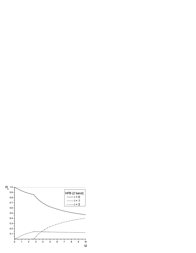
Figure 1: Atomic fractions, as functions of the dimensionless interaction parameter $u$, for the condensed atoms (solid line), uncondensed atoms (dotted line), and localized atoms (dashed-dotted line).

References

• [1] D. Jaksch and P. Zoller, Ann. Phys. (N.Y.) 315, 52 (2005).
• [2] O. Morsch and M. Oberthaler, Rev. Mod. Phys. 78, 179 (2006).
• [3] C. Moseley, O. Fialko, and K. Ziegler, Ann. Physik 17, 561 (2008).
• [4] I. Bloch, J. Dalibard, and W. Zwerger, Rev. Mod. Phys. 80, 885 (2008).
• [5] V.I. Yukalov, Laser Phys. 19, 1 (2009).
• [6] J.K. Freericks and H. Monien, Phys. Rev. B 53, 2691 (1996).
• [7] N. Elstner and H. Monien, Phys. Rev. B 59, 12184 (1999).
• [8] S. Wessel, F. Alet, M. Troyer, and G.G. Batrouni, Phys. Rev. A 70, 053615 (2004).
• [9] B. Capogrosso-Sansone, N. V. Prokofiev, and B. V. Svistunov, Phys. Rev. B 75, 134302 (2007).
• [10] B. Capogrosso-Sansone, S.G. SΓΆyler, N. Prokofiev, and B. Svistunov, Phys. Rev. A 77, 015602 (2008).
• [11] D.B. Dickerscheid, D. van Oosten, P.J. Denteneer, and H.T.C. Stoof, Phys. Rev. A 68, 043623 (2003).
• [12] A. E. Meyerovich, Phys. Rev. A 68, 051602 (2003).
• [13] L. I. Plimak, M. K. Olsen, and M. Fleischhauer, Phys. Rev. A 70, 013611 (2004).
• [14] F. Gerbier, Phys. Rev. Lett. 99, 120405 (2007).
• [15] V.I. Yukalov and E.P. Yukalova, Phys. Rev. A 78, 063610 (2008).
• [16] V.I. Yukalov and E.P. Yukalova, Laser Phys. Lett. 6, 235 (2009).
• [17] V.I. Yukalov and E.P. Yukalova, Phys. Lett. A 373, 1301 (2009).
• [18] F.A. Buot, Phys. Rep. 234, 73 (1993).
• [19] V.I. Yukalov, Ann. Physik 36, 31 (1979).
• [20] V.I. Yukalov, Ann. Physik 38, 419 (1981).
• [21] V.I. Yukalov and V.I. Zubov, Fortschr. Phys. 31, 627 (1983).
• [22] V.I. Yukalov, Physica A 89, 363 (1977).
• [23] D.I. Pushkarov, Quasiparticle Theory of Defects in Solids (World Scientific, Singapore, 1991).
• [24] N.N. Bogolubov, Lectures on Quantum Statistics (Gordon and Breach, New York, 1970), Vol. 2.
• [25] V.I. Yukalov, Phys. Rev. E 72, 066119 (2005).
• [26] V.I. Yukalov, Laser Phys. 16, 511 (2006).
• [27] V.I. Yukalov, Int. J. Mod. Phys. B 21, 69 (2007).
• [28] V.I. Yukalov, Phys. Lett. A 359, 712 (2006).
• [29] V.I. Yukalov, Laser Phys. Lett. 3, 406 (2006).
• [30] V.I. Yukalov, Ann. Phys. (N.Y.) 323, 461 (2008).
• [31] V.I. Yukalov and H. Kleinert, Phys. Rev. A 73, 063612 (2006).
• [32] V.I. Yukalov and E.P. Yukalova, Phys. Rev. A 74, 063623 (2006).
• [33] V.I. Yukalov and E.P. Yukalova, Phys. Rev. A 76, 013602 (2007).
• [34] A. Rakhimov, C.K. Kim, S.H. Kim, and J.H. Yee, Phys. Rev. A 77, 033626 (2008).
• [35] A. Rakhimov, E.Y. Sherman, and C.K. Kim, Phys. Rev. B 81, 020407 (2010).
• [36] N.M. Hugenholtz and D. Pines, Phys. Rev. 116, 489 (1959).
• [37] I. Danshita and P. Naidon, Phys. Rev. A 79, 043601 (2009).
• [38] V.I. Yukalov and M.D. Girardeau, Laser Phys. Lett. 2, 375 (2005).
• [39] F. Cinty, P. Jain, M. Boninsegni, A. Micheli, P. Zoller, and G. Pupillo, arXiv:1005.2403 (2010).
• [40] K.P. Marzlin and V.I. Yukalov, Eur. Phys. J. D 33, 253 (2005).
• [41] V.O. Nesterenko, A.N. Novikov, F.F. de Souza Cruz, and E.L. Lapolli, Laser Phys. 19, 616 (2009).
• [42] L.Y. Yang, L.B. Fu, and J. Liu, Laser Phys. 19, 678 (2009).
• [43] V.I. Yukalov, E.P. Yukalova, and V.S. Bagnato, Laser Phys. 19, 686 (2009).
• [44] A. Zenesini, H. Lignier, C. Sias, O. Morsch, D. Ciampini, and E. Arimondo, Laser Phys. 20, 1182 (2010).
• [45] V.I. Yukalov, Laser Phys. Lett. 7, 467 (2010).