Vacuum structure and chiral symmetry breaking in strong magnetic fields for hot and dense quark matter

Abstract

We investigate chiral symmetry breaking in strong magnetic fields at finite temperature and densities in a 3 flavor Nambu Jona Lasinio (NJL) model including the Kobayashi Maskawa t-Hooft (KMT) determinant term, using an explicit structure for the ground state in terms of quark antiquark condensates. The mass gap equations are solved self consistently and are used to compute the thermodynamic potential. We also derive the equation of state for strange quark matter in the presence of strong magnetic fields which could be relevant for proto-neutron stars.

I Introduction

The structure of QCD vacuum and its modification under extreme environment has been a major theoretical and experimental challenge in current physics review . In particular, it is interesting to study the modification of the structure of ground state at high temperature and/or high baryon densities as related to the nonperturbative aspects of QCD. This is important not only from a theoretical point of view, but also for many applications to problems of quark gluon plasma that could be copiously produced in relativistic heavy ion collisions as well as for the ultra dense cold nuclear/quark matter which could be present in the interior of compact stellar objects like neutron stars. In addition to hot and dense QCD, the effect of strong magnetic field on QCD vacuum structure has attracted recent attention.This is motivated by the possibility of creating ultra strong magnetic fields in non central collisions at RHIC and LHC. The strengths of the magnetic fields are estimated to be of hadronic scale larrywarringa ; skokov of the order of $eB\sim 2m_{\pi}^{2}$ ($m_{\pi}^{2}\simeq 10^{18}$ Gauss) at RHIC, to about $eB\sim 15m_{\pi}^{2}$ at LHC skokov .

There have been recent calculations both analytic as well as with lattice simulations, which indicate that QCD phase digram is affected by strong magnetic fields dima ; maglat ; fraga . One of the interesting findings has been the chiral magnetic effect. Here an electric current of quarks along the magnetic field axis is generated if the densities of left and right handed quarks are not equal. At high temperatures and in presence of magnetic field such a current can be produced locally. The phase structure of dense matter in presence of magnetic field along with a non zero chiral density has recently been investigated for two flavor PNJL model for high temperatures relevant for RHIC and LHC fukushimaplb . There have also been many investigations to look into the vacuum structure of QCD and it has been recognized that the strong magnetic field acts as a catalyser of chiral symmetry breaking igormag ; miranski ; klimenko ; boomsma .

In the context of cold dense matter, compact stars can be strongly magnetized. Neutron star observations indicate the magnetic field to be of the order of $10^{12}$-$10^{13}$ Gauss at the surface of ordinary pulsars somenath . Further, the magnetars which are strongly magnetized neutron stars, may have even stronger magnetic fields of the order of $10^{15}-10^{16}$ Gauss dunc ; duncc ; dunccc ; duncccc ; lat ; broder ; lai . Physical upper limit on the magnetic field in a gravitationally bound star is $10^{18}$ Gauss that is obtained by comparing the magnetic and gravitational energies using virial theorem somenath . This limit could be higher for self bound objects like quark stars ferrer3 . Since the magnetic field strengths are of the order of QCD scale, this can affect both the thermodynamic as well as hydrodynamics of such magnetized matter armendirk . The effects of magnetic field on the equation of state have been recently studied in Nambu Jona Lasinio model at zero temperature for three flavors and the equation of state has been computed for the cold quark matter providencia . It will be interesting to consider the finite temperature effects on such equation of state, which could be of relevance for proto-neutron stars.

We had earlier considered a variational approach to study chiral symmetry breaking as well as color superconductivity in hot and dense matter with an explicit structure for the ‘ground state’ hmspmnjl ; hmparikh ; hmam . The calculations were carried out within NJL model with minimization of free energy density to decide which condensate will exist at what density and/or temperature. A nice feature of the approach is that the four component quark field operator in the chiral symmetry broken phase gets determined from the vacuum structure. In the present work, we aim to investigate how the vacuum structure in the context of chiral symmetry breaking gets modified in the presence of magnetic field.

We organize the paper as follows. In section II, we discuss the ansatz state with quark antiquark pairs in the presence of a magnetic field. We then generalize such a state to include the effects of temperature and density. In section III, we consider the 3 flavor NJL model along with the so called KMT term–the six fermion determinant interaction term which breaks U(1) axial symmetry as in QCD. We use this Hamiltonian and calculate its expectation value with respect to the ansatz state to compute the energy density as well the thermodynamic potential for this system. We minimize the thermodynamic potential to determine the the ansatz functions and the resulting mass gap equations. We discuss the results of the present investigation in section IV. Finally we summarize and conclude in section V. For the sake of completeness we derive the spinors in the presence of a magnetic field and some of their properties, which are presented in the appendix.

II The ansatz for the ground state

To make the notations clear, we first write down the field operator expansion in the momentum space in the presence of a constant magnetic field ${\bf{B}}$ in the $z-$ direction for a quark with a current mass $m$ and electric charge $q$. We choose the gauge such that the electromagnetic vector potential is given as $A_{\mu}(\mathchoice{\mbox{\boldmath$x$}}{\mbox{\boldmath$x$}}{\mbox{\boldmath$\scriptstyle x$}}{\mbox{\boldmath$\scriptscriptstyle x$}})=(0,0,Bx,0)$. The Dirac field operator for a particle is given as kausik

$$\psi({\bf{x}})=\sum_{n}\sum_{r}\frac{1}{2\pi}\int{d{\bf{p}}_{{}_{\!\hbox to0.0pt{$\scriptscriptstyle\backslash$\hss}{\scriptscriptstyle x}}}\left[q_{r}(n,{\bf{p}}_{{}_{\!\hbox to0.0pt{$\scriptscriptstyle\backslash$\hss}{\scriptscriptstyle x}}})U_{r}(x,{\bf{p}}_{{}_{\!\hbox to0.0pt{$\scriptscriptstyle\backslash$\hss}{\scriptscriptstyle x}}},n)+\tilde{q}_{r}(n,-{\bf{p}}_{{}_{\!\hbox to0.0pt{$\scriptscriptstyle\backslash$\hss}{\scriptscriptstyle x}}})V_{r}(x,-{\bf{p}}_{{}_{\!\hbox to0.0pt{$\scriptscriptstyle\backslash$\hss}{\scriptscriptstyle x}}},n)\right]e^{i{\bf{p}}_{{}_{\!\hbox to0.0pt{$\scriptscriptstyle\backslash$\hss}{\scriptscriptstyle x}}}\cdot{\bf{x}}_{{}_{\!\hbox to0.0pt{$\scriptscriptstyle\backslash$\hss}{\scriptscriptstyle x}}}}}.$$ (1)

The sum over $n$ in the above expansion runs from 0 to infinity. In the above, ${\bf{p}}_{{}_{\!\hbox to0.0pt{$\scriptscriptstyle\backslash$\hss}{\scriptscriptstyle x}}}\equiv(p_{y},p_{z})$, and, $r=\pm 1$ denotes the up and down spins. We have suppressed the color and flavor indices of the quark field operators. The quark annihilation and antiquark creation operators, $q_{r}$ and $\tilde{q}_{r}$, respectively, satisfy the quantum algebra

$$\{q_{r}(n,{\bf{p}}_{{}_{\!\hbox to0.0pt{$\scriptscriptstyle\backslash$\hss}{\scriptscriptstyle x}}}),q_{r^{\prime}}^{\dagger}(n^{\prime},{\bf{p}}_{{}_{\!\hbox to0.0pt{$\scriptscriptstyle\backslash$\hss}{\scriptscriptstyle x}}}^{\prime})\}=\{\tilde{q}_{r}(n,{\bf{p}}_{{}_{\!\hbox to0.0pt{$\scriptscriptstyle\backslash$\hss}{\scriptscriptstyle x}}}),\tilde{q}_{r^{\prime}}^{\dagger}(n^{\prime},{\bf{p}}_{{}_{\!\hbox to0.0pt{$\scriptscriptstyle\backslash$\hss}{\scriptscriptstyle x}}}^{\prime})\}=\delta_{rr^{\prime}}\delta_{nn^{\prime}}\delta({\bf{p}}_{{}_{\!\hbox to0.0pt{$\scriptscriptstyle\backslash$\hss}{\scriptscriptstyle x}}}-{\bf{p}}_{{}_{\!\hbox to0.0pt{$\scriptscriptstyle\backslash$\hss}{\scriptscriptstyle x}}}^{\prime}).$$ (2)

In the above, $U_{r}$ and $V_{r}$ are the four component spinors for the quarks and antiquarks respectively. The explicit forms of the spinors for the fermions with mass $m$ and electric charge $q$ are given by

$$U_{\uparrow}(x,\mathchoice{\mbox{\boldmath$p$}}{\mbox{\boldmath$p$}}{\mbox{\boldmath$\scriptstyle p$}}{\mbox{\boldmath$\scriptscriptstyle p$}}_{{}_{\!\hbox to0.0pt{$\scriptscriptstyle\backslash$\hss}{\scriptscriptstyle x}}},n) = \frac{1}{\sqrt{2\epsilon_{n}(\epsilon_{n}+m)}}\left(\begin{array}[]{c}(\epsilon_{n}+m)\left(\Theta(q)I_{n}+\Theta(-q)I_{n-1}\right)\\ 0\\ p_{z}\left(\Theta(q)I_{n}+\Theta(-q)I_{n-1}\right)\\ -i\sqrt{2n|q|B}\left(\Theta(q)I_{n-1}+\Theta(-q)I_{n}\right)\\ \end{array}\right)$$ (3e)

$$U_{\downarrow}(x,\mathchoice{\mbox{\boldmath$p$}}{\mbox{\boldmath$p$}}{\mbox{\boldmath$\scriptstyle p$}}{\mbox{\boldmath$\scriptscriptstyle p$}}_{{}_{\!\hbox to0.0pt{$\scriptscriptstyle\backslash$\hss}{\scriptscriptstyle x}}},n) = \frac{1}{\sqrt{2\epsilon_{n}(\epsilon_{n}+m)}}\left(\begin{array}[]{c}0\\ (\epsilon_{n}+m)\left(\Theta(q)I_{n-1}+\Theta(-q)I_{n}\right)\\ i\sqrt{2n|q|B}\left(\Theta(q)I_{n}-\Theta(-q)I_{n-1}\right)\\ -p_{z}\left(\Theta(q)I_{n}-\Theta(-q)I_{n-1}\right)\\ \end{array}\right)$$ (3j)

$$V_{\uparrow}(x,-{\bf{p}}_{{}_{\!\hbox to0.0pt{$\scriptscriptstyle\backslash$\hss}{\scriptscriptstyle x}}},n) = \frac{1}{\sqrt{2\epsilon_{n}(\epsilon_{n}+m)}}\left(\begin{array}[]{c}\sqrt{2n|q|B}\left(\Theta(q)I_{n}-\Theta(-q)I_{n-1}\right)\\ ip_{z}\left(\Theta(q)I_{n-1}+\Theta(-q)I_{n}\right)\\ 0\\ i(\epsilon_{n}+m)\left(\Theta(q)I_{n-1}+\Theta(-q)I_{n}\right)\\ \end{array}\right)$$ (3o)

$$V_{\downarrow}(x,-\mathchoice{\mbox{\boldmath$p$}}{\mbox{\boldmath$p$}}{\mbox{\boldmath$\scriptstyle p$}}{\mbox{\boldmath$\scriptscriptstyle p$}}_{{}_{\!\hbox to0.0pt{$\scriptscriptstyle\backslash$\hss}{\scriptscriptstyle x}}},n) = \frac{1}{\sqrt{2\epsilon_{n}(\epsilon_{n}+m)}}\left(\begin{array}[]{c}ip_{z}\left(\Theta(q)I_{n}+\Theta(-q)I_{n-1}\right)\\ \sqrt{2n|q|B}\left(\Theta(q)I_{n-1}-\Theta(-q)I_{n-1}\right)\\ -i(\epsilon_{n}+m)\left(\Theta(q)I_{n}+\Theta(-q)I_{n-1}\right)\\ 0\\ \end{array}\right).$$ (3t)

In the above, the energy of the n-th Landau level is given as $\epsilon_{n}=\sqrt{m_{i}^{2}+p_{z}^{2}+2n|q_{i}|B}\equiv\sqrt{m_{i}^{2}+|{\bf{p}}_{i}^{2}|}$. In Eq.s (3), the functions $I_{n}`$s (with $n\geq 0$) are functions of $\xi=|q_{i}B|(x-p_{y}/|q_{i}B|)$ and are given as

$$I_{n}(\xi)=c_{n}\exp\left(-\frac{\xi^{2}}{2}\right)H_{n}(\xi)$$ (4)

where, $H_{n}(\xi)$ is the Hermite polynomial of the nth order and $I_{-1}=0$. The normalization constant $c_{n}$ is given by

$$c_{n}=\sqrt{\frac{\sqrt{|q|B}}{n!2^{n}\sqrt{\pi}}}$$

The functions $I_{n}(\xi)$ satisfy the orthonormality condition

$$\int{d\xi I_{n}(\xi)I_{m}(\xi)}=\sqrt{|q|B}\delta_{n,m}$$ (5)

so that the spinors are properly normalized. The detailed derivation of these spinors and some of their properties are presented in the appendix.

With the field operators now defined in terms of the annihilation and the creation operators in presence of a constant magnetic field, we now write down an ansatz for the ground state taken as a squeezed coherent state involving quark and antiquarks pairs as amhm5 ; hmam ; hmparikh

$$|\Omega\rangle={\cal U}_{Q}|0\rangle.$$ (6)

Here, ${\cal U}_{Q}$ is an unitary operator which creates quark–antiquark pairs from the vacuum $|0\rangle$. Explicitly, the operator, ${\cal U}_{Q}$ is given as

$${\cal U}_{Q}=\exp\left(\sum_{n=0}^{\infty}\int{d\mathchoice{\mbox{\boldmath$p$}}{\mbox{\boldmath$p$}}{\mbox{\boldmath$\scriptstyle p$}}{\mbox{\boldmath$\scriptscriptstyle p$}}_{{}_{\!\hbox to0.0pt{$\scriptscriptstyle\backslash$\hss}{\scriptscriptstyle x}}}{q_{r}^{i}}^{\dagger}(n,\mathchoice{\mbox{\boldmath$p$}}{\mbox{\boldmath$p$}}{\mbox{\boldmath$\scriptstyle p$}}{\mbox{\boldmath$\scriptscriptstyle p$}}_{{}_{\!\hbox to0.0pt{$\scriptscriptstyle\backslash$\hss}{\scriptscriptstyle x}}})a_{r,s}^{i}(n,p_{z})f^{i}(n,\mathchoice{\mbox{\boldmath$p$}}{\mbox{\boldmath$p$}}{\mbox{\boldmath$\scriptstyle p$}}{\mbox{\boldmath$\scriptscriptstyle p$}}_{{}_{\!\hbox to0.0pt{$\scriptscriptstyle\backslash$\hss}{\scriptscriptstyle x}}})\tilde{q}_{s}^{i}(n,-\mathchoice{\mbox{\boldmath$p$}}{\mbox{\boldmath$p$}}{\mbox{\boldmath$\scriptstyle p$}}{\mbox{\boldmath$\scriptscriptstyle p$}}_{{}_{\!\hbox to0.0pt{$\scriptscriptstyle\backslash$\hss}{\scriptscriptstyle x}}})}-h.c.\right)$$ (7)

where, we have explicitly retained the flavor index $i$ for the quark field operators. In the above ansatz for the ground state, $f^{i}(n,p_{z})$ is a real function describing the quark antiquark condensates related to the vacuum realignment for chiral symmetry breaking. In the above equation, the spin dependent structure $a_{r,s}^{i}$ is given by

$$a_{r,s}^{i}=\frac{1}{|{\bf{p}}_{i}|}\left[-\sqrt{2n|q_{i}|B}\delta_{r,s}-ip_{z}\delta_{r,-s}\right]$$ (8)

with $|{\bf{p}}_{i}|=\sqrt{p_{z}^{2}+2n|q_{i}|B}$ denoting the magnitude of the three momentum of the quark/antiquark of $i$-th flavor (with electric charge $q_{i}$) in presence of a magnetic field. It is easy to show that, $aa^{\dagger}=I$, where $I$ is an identity matrix in two dimensions. The ansatz functions $f_{i}(n,p_{z})$ are determined from the minimization of thermodynamic potential. This particular ansatz of Eq.(7) is a direct generalization of the ansatz considered earlier hmspmnjl ; hmam , to include the effects of magnetic field. Clearly, a nontrivial $f_{i}(n,p_{z})$ breaks the chiral symmetry. Summation over three colors is understood in the exponent of ${\cal U}_{Q}$ in Eq. (7).

It is easy to show that the transformation of the ground state as in Eq.(6) is a Bogoliubov transformation. With the ground state transforming as Eq.(6), any operator $O$ in the $|0\rangle$ basis transforms as

$$O^{\prime}={\cal U}_{Q}O{\cal U}_{Q}^{\dagger}$$ (9)

and, in particular, the creation and the annihilation operators of Eq.(1) transform as

$$\left[\begin{array}[]{c}q_{r}^{\prime}(n,{\bf{p}}_{{}_{\!\hbox to0.0pt{$\scriptscriptstyle\backslash$\hss}{\scriptscriptstyle x}}})\\ \tilde{q}_{s}^{\prime}(n,-{\bf{p}}_{{}_{\!\hbox to0.0pt{$\scriptscriptstyle\backslash$\hss}{\scriptscriptstyle x}}})\end{array}\right] = U_{Q}\left[\begin{array}[]{c}q_{r}(n,{\bf{p}}_{{}_{\!\hbox to0.0pt{$\scriptscriptstyle\backslash$\hss}{\scriptscriptstyle x}}})\\ \tilde{q}_{s}(n,-{\bf{p}}_{{}_{\!\hbox to0.0pt{$\scriptscriptstyle\backslash$\hss}{\scriptscriptstyle x}}})\end{array}\right]U_{Q}^{\dagger}$$ (14)

$$= \left[\begin{array}[]{cc}\cos|f|&-a_{r,s}\sin|f|\\ a^{\dagger}_{s,r}\sin|f|&\cos|f|\end{array}\right]\left[\begin{array}[]{c}q_{r}(n,{\bf{p}}_{{}_{\!\hbox to0.0pt{$\scriptscriptstyle\backslash$\hss}{\scriptscriptstyle x}}})\\ \tilde{q}_{s}(n,-{\bf{p}}_{{}_{\!\hbox to0.0pt{$\scriptscriptstyle\backslash$\hss}{\scriptscriptstyle x}}})\end{array}\right],$$ (19)

which is a Bogoliubov transformation with the transformed ‘primed’ operators satisfying the same anti-commutation relations as the ‘unprimed’ ones as in Eq.(2). Using the transformation Eq. (LABEL:bogtrans), we can expand the quark field operator $\psi({\bf{x}})$ in terms of the primed operators given as,

$$\psi({\bf{x}})=\sum_{n}\sum_{r}\frac{1}{2\pi}\int{d{\bf{p}}_{{}_{\!\hbox to0.0pt{$\scriptscriptstyle\backslash$\hss}{\scriptscriptstyle x}}}\left[q_{r}^{\prime}(n,{\bf{p}}_{{}_{\!\hbox to0.0pt{$\scriptscriptstyle\backslash$\hss}{\scriptscriptstyle x}}})U_{r}^{\prime}(x,n,{\bf{p}}_{{}_{\!\hbox to0.0pt{$\scriptscriptstyle\backslash$\hss}{\scriptscriptstyle x}}})+\tilde{q}_{r}^{\prime}(n,-{\bf{p}}_{{}_{\!\hbox to0.0pt{$\scriptscriptstyle\backslash$\hss}{\scriptscriptstyle x}}})V_{r}^{\prime}(x,n,-{\bf{p}}_{{}_{\!\hbox to0.0pt{$\scriptscriptstyle\backslash$\hss}{\scriptscriptstyle x}}})\right]e^{i{\bf{p}}_{{}_{\!\hbox to0.0pt{$\scriptscriptstyle\backslash$\hss}{\scriptscriptstyle x}}}\cdot{\bf{x}}_{{}_{\!\hbox to0.0pt{$\scriptscriptstyle\backslash$\hss}{\scriptscriptstyle x}}}}},$$ (20)

with $q^{\prime}|\Omega\rangle=0={\tilde{q}}^{\prime{\dagger}}|\Omega\rangle$. In the above, we have suppressed the flavor and color indices. It is easy to see that the ‘primed’ spinors are give as

$$U_{r}^{\prime}(x,n,p_{{}_{\!\hbox to0.0pt{$\scriptscriptstyle\backslash$\hss}{\scriptscriptstyle x}}})=\cos|f|U_{r}(x,n,p_{{}_{\!\hbox to0.0pt{$\scriptscriptstyle\backslash$\hss}{\scriptscriptstyle x}}})-a_{r,s}^{\dagger}\sin|f|V_{s}(x,n,-p_{{}_{\!\hbox to0.0pt{$\scriptscriptstyle\backslash$\hss}{\scriptscriptstyle x}}})$$ (21a)

$$V_{r}^{\prime}(x,n,-p_{{}_{\!\hbox to0.0pt{$\scriptscriptstyle\backslash$\hss}{\scriptscriptstyle x}}})=\cos|f|V_{r}(x,n,-p_{{}_{\!\hbox to0.0pt{$\scriptscriptstyle\backslash$\hss}{\scriptscriptstyle x}}})+a_{s,r}\sin|f|U_{s}(x,n,p_{{}_{\!\hbox to0.0pt{$\scriptscriptstyle\backslash$\hss}{\scriptscriptstyle x}}}).$$ (21b)

Explicit calculation, e.g. for positive charges yield the following forms of the primed spinors:

$$U_{\uparrow}^{\prime}(\mathchoice{\mbox{\boldmath$p$}}{\mbox{\boldmath$p$}}{\mbox{\boldmath$\scriptstyle p$}}{\mbox{\boldmath$\scriptscriptstyle p$}}_{{}_{\!\hbox to0.0pt{$\scriptscriptstyle\backslash$\hss}{\scriptscriptstyle x}}},n) = \frac{1}{\sqrt{2\epsilon_{n}(\epsilon_{n}+m)}}\left[\begin{array}[]{c}a_{1}I_{n}\\ 0\\ a_{2}p_{z}I_{n}\\ -ia_{2}\sqrt{2n|q|B}I_{n-1}\\ \end{array}\right]$$ (22e)

$$U_{\downarrow}^{\prime}(\mathchoice{\mbox{\boldmath$p$}}{\mbox{\boldmath$p$}}{\mbox{\boldmath$\scriptstyle p$}}{\mbox{\boldmath$\scriptscriptstyle p$}}_{{}_{\!\hbox to0.0pt{$\scriptscriptstyle\backslash$\hss}{\scriptscriptstyle x}}},n) = \frac{1}{\sqrt{2\epsilon_{n}(\epsilon_{n}+m)}}\left[\begin{array}[]{c}0\\ a_{1}I_{n-1}\\ ia_{2}\sqrt{2n|q|B}I_{n}\\ -a_{2}p_{z}I_{n-1}\\ \end{array}\right]$$ (22j)

$$V_{\uparrow}^{\prime}(-\mathchoice{\mbox{\boldmath$p$}}{\mbox{\boldmath$p$}}{\mbox{\boldmath$\scriptstyle p$}}{\mbox{\boldmath$\scriptscriptstyle p$}}_{{}_{\!\hbox to0.0pt{$\scriptscriptstyle\backslash$\hss}{\scriptscriptstyle x}}},n) = \frac{1}{\sqrt{2\epsilon_{n}(\epsilon_{n}+m)}}\left[\begin{array}[]{c}a_{2}\sqrt{2n|q|B}I_{n}\\ ia_{2}p_{z}I_{n-1}\\ 0\\ ia_{1}I_{n-1}\\ \end{array}\right]$$ (22o)

$$V_{\downarrow}^{\prime}(-\mathchoice{\mbox{\boldmath$p$}}{\mbox{\boldmath$p$}}{\mbox{\boldmath$\scriptstyle p$}}{\mbox{\boldmath$\scriptscriptstyle p$}}_{{}_{\!\hbox to0.0pt{$\scriptscriptstyle\backslash$\hss}{\scriptscriptstyle x}}},n) = \frac{1}{\sqrt{2\epsilon_{n}(\epsilon_{n}+m)}}\left[\begin{array}[]{c}ia_{2}p_{z}I_{n}\\ a_{2}\sqrt{2n|q|B}I_{n-1}\\ -ia_{1}I_{n}\\ 0\\ \end{array}\right],$$ (22t)

where the functions, $a_{1}$ and $a_{2}$, are given in terms of the condensate function $f(p_{z},n)$ as

$$a_{1} = (\epsilon_{n}+m)\cos|f(n,p_{z})|+|{\bf{p}}_{i}|\sin|f(n,p_{z})|$$ (23)

$$a_{2} = \cos|f(n,p_{z})|-\frac{\epsilon_{n}+m}{|{\bf{p}}_{i}|}\sin|f(n,p_{z})|,$$ (24)

Let us note that with Eq.(20), the four component quark field operator gets defined in terms of the vacuum structure for chiral symmetry breaking given through Eq.(6) and Eq.(7) amspm ; spmindianj .

To include the effects of temperature and density we next write down the state at finite temperature and density $|\Omega(\beta,\mu)\rangle$ through a thermal Bogoliubov transformation over the state $|\Omega\rangle$ using the thermo field dynamics (TFD) method as described in Ref.s tfd ; amph4 . This is particularly useful while dealing with operators and expectation values. We write the thermal state as

$$|\Omega(\beta,\mu)\rangle={\cal U}_{\beta,\mu}|\Omega\rangle={\cal U}_{\beta,\mu}{\cal U}_{Q}|0\rangle,$$ (25)

where ${\cal U}_{\beta,\mu}$ is given as

$${\cal U}_{\beta,\mu}=e^{{\cal B}^{\dagger}(\beta,\mu)-{\cal B}(\beta,\mu)},$$

with

$${\cal B}^{\dagger}(\beta,\mu)=\int\Big{[}\sum_{n=0}^{\infty}\int d\mathchoice{\mbox{\boldmath$k$}}{\mbox{\boldmath$k$}}{\mbox{\boldmath$\scriptstyle k$}}{\mbox{\boldmath$\scriptscriptstyle k$}}_{{}_{\!\hbox to0.0pt{$\scriptscriptstyle\backslash$\hss}{\scriptscriptstyle x}}}q_{r}^{\prime}(n,k_{z})^{\dagger}\theta_{-}(k_{z},n,\beta,\mu)\underline{q}_{r}^{\prime}(n,k_{z})^{\dagger}+\tilde{q}_{r}^{\prime}(n,k_{z})\theta_{+}(k_{z},n,\beta,\mu)\underline{\tilde{q}}_{r}^{\prime}(n,k_{z})\Big{]}.$$ (26)

In Eq.(26), the underlined operators are the operators in the extended Hilbert space associated with thermal doubling in TFD method, and, the ansatz functions $\theta_{\pm}(n,k_{z},\beta,\mu)$ are related to quark and antiquark distributions as can be seen through the minimization of the thermodynamic potential. In Eq.(26) we have suppressed the color and flavor indices in the quark and antiquark operators as well as in the functions $\theta_{\mp}$.

All the functions in the ansatz in Eq.(25) are obtained by minimizing the thermodynamic potential. We shall carry out this minimization in the next section. However, before carrying out the minimization procedure, let us focus our attention to the expectation values of some known operators to show that with the above variational ansatz for the ‘ground state’ given in Eq.(25) these reduce to the already known expressions in the appropriate limits.

Let us first consider the expectation value of the chiral order parameter. The expectation value for chiral order parameter for the $i$-th flavor is given as

$$\langle\Omega(\beta,\mu)|\bar{\psi}_{i}\psi_{i}|\Omega(\beta,\mu)\rangle = -\sum_{n=0}^{\infty}\frac{N_{c}|q_{i}|B\alpha_{n}}{(2\pi)^{2}}\int{\frac{dp_{z}}{\epsilon_{ni}}\left[m_{i}\cos{2f_{i}}+|{\bf{p}}_{i}|\sin{2f_{i}}\right]}\left(1-\sin^{2}\theta_{-}^{i}-\sin^{2}\theta_{+}^{i}\right)$$ (27)

$$\equiv -I^{i}$$

where, $\alpha_{n}=(2-\delta_{n,0})$ is the degeneracy factor of the $n$-th Landau level (all levels are doubly degenerate except the lowest Landau level). As we shall see later, the functions $\sin^{2}\theta_{\mp}$ will be related to the distribution functions for the quarks and antiquarks. Further, for later convenience, it is useful to define $\cos\phi_{0}^{i}=m_{i}/\epsilon_{ni}$ and $\sin\phi_{0}^{i}=|{\bf{p}}_{i}|/\epsilon_{ni}$ so as to rewrite the order parameter $I_{i}$ as

$$I_{i}=\sum_{n=0}^{\infty}\frac{N_{c}|q_{i}|B\alpha_{n}}{(2\pi)^{2}}\int{dp_{z}}\cos\phi^{i}\left(1-\sin^{2}\theta_{-}^{i}-\sin^{2}\theta_{+}^{i}\right),$$ (28)

where we have defined $\phi^{i}=\phi_{0}^{i}-2f_{i}$. As we shall see later, it is convenient to vary $\phi^{i}$ as compared to the original condensate function $f_{i}$ given through Eq.(7). This expression for the order parameter, $I_{i}$, in the limit of vanishing condensates ($f_{i}$=0) reduces to the expression derived in Ref. kausik . Further, the expression for the chiral condensate in the absence of the magnetic field at zero temperature and zero density becomes

$$\langle\bar{\psi}^{i}\psi^{i}\rangle=-I_{i}=-\frac{6}{(2\pi)^{3}}\int d{\bf{p}}\cos\phi^{i},$$ (29)

once one realizes that in presence of quantizing magnetic field with discrete Landau levels, one has digal

$$\int\frac{d{\bf{p}}}{(2\pi)^{3}}\rightarrow\frac{|qB|}{(2\pi)^{2}}\sum_{n=0}^{\infty}\alpha_{n}\int dp_{z}.$$

This expression for the condensate, Eq.(29) is exactly the same as derived earlier in the absence of the magnetic field hmspmnjl ; hmam .

The other quantity that we wish to investigate is the axial fermion current density that is induced at finite chemical potential including the effect of temperature. The expectation value of the axial current density is given by

$$\langle j_{5}^{3}\rangle\equiv\langle\bar{\psi_{i}^{a}}\gamma^{3}\gamma^{5}\psi_{j}^{a}\rangle.$$

Using the field operator expansion Eq.(20) and Eq.(22t) for the explicit forms for the spinors, we have for the $i$-th flavor

$$\langle j_{5}^{i3}\rangle=\sum_{n}\frac{N_{c}}{(2\pi)^{2}}\int{dp_{{}_{\!\hbox to0.0pt{$\scriptscriptstyle\backslash$\hss}{\scriptscriptstyle x}}}\left(I_{n}^{2}-I_{n-1}^{2}\right)\left(\sin^{2}\theta_{-}^{i}-\sin^{2}\theta_{+}^{i}\right)}.$$ (30)

Integrating over $dp_{y}$ using the orthonormal condition of Eq.(5), all the terms in the above sum for the Landau levels cancel out except for the zeroth Landau level so that,

$$\langle j_{5}^{i3}\rangle=\frac{N_{c}|q_{i}|B}{(2\pi)^{2}}\int{dp_{z}\left[\sin^{2}\theta_{-}^{i0}-\sin^{2}\theta_{+}^{i0}\right]}.$$ (31)

which is identical to that in Ref.metlitsky once we identify the functions $\sin^{2}\theta_{\mp}^{i0}$ as the particle and the antiparticle distribution functions for the zero modes (see e.g. Eq.(42) in the next section).

III Evaluation of thermodynamic potential and gap equations

As has already been mentioned, we shall consider in the present investigation, the 3-flavor Nambu Jona Lasinio model including the Kobayashi-Maskawa-t-Hooft (KMT) determinant interaction. The corresponding Hamiltonian density is given as

$${\cal H} = \psi^{\dagger}(-i\mbox{\boldmath$\alpha$}\cdot\mbox{\boldmath$\nabla$}-qBx\alpha_{2}+\gamma^{0}\hat{m})\psi-G_{s}\sum_{A=0}^{8}\left[(\bar{\psi}\lambda^{A}\psi)^{2}-(\bar{\psi}\gamma^{5}\lambda^{A}\psi)^{2}\right]$$ (32)

$$+ K\left[{det_{f}[\bar{\psi}(1+\gamma_{5})\psi]+det_{f}[\bar{\psi}(1-\gamma_{5})\psi]}\right]$$

where $\psi^{i,a}$ denotes a quark field with color ‘$a$’ $(a=r,g,b)$, and flavor ‘$i$’ $(i=u,d,s)$, indices. The matrix of current quark masses is given by $\hat{m}$=diag${}_{f}(m_{u},m_{d},m_{s})$ in the flavor space. We shall assume in the present investigation, isospin symmetry with $m_{u}$=$m_{d}$. Strictly speaking, when the electromagnetic effects are taken into account, the current quark masses of u and d quarks should not be the same due to the difference in their electrical charges. However, because of the smallness of the electromagnetic coupling, we shall ignore this tiny effect and continue with $m_{u}=m_{d}$ in the present investigation of chiral symmetry breaking. In Eq. (32), $\lambda^{A}$, $A=1,\cdots 8$ denote the Gellman matrices acting in the flavor space and $\lambda^{0}=\sqrt{\frac{2}{3}}\,11_{f}$, $11_{f}$ as the unit matrix in the flavor space. The four point interaction term $\sim G_{s}$ is symmetric in $SU(3)_{V}\times SU(3)_{A}\times U(1)_{V}\times U(1)_{A}$. In contrast, the determinant term $\sim K$ which for the case of three flavors generates a six point interaction breaks $U(1)_{A}$ symmetry. In the absence of the magnetic field and the mass term, the overall symmetry in the flavor space is $SU(3)_{V}\times SU(3)_{A}\times U(1)_{V}$. This spontaneously breaks to $SU(3)_{V}\times U(1)_{V}$ implying the conservation of the baryon number and the flavor number. The current quark mass term introduces additional explicit breaking of chiral symmetry leading to partial conservation of the axial current. Due to the presence of magnetic field on the other hand the $SU(3)_{V}$ symmetry in the flavor space reduces to to $SU(2)_{V}\times SU(2)_{A}$ since the u quark has different electric charge compared to d and s quarks manfer .

Next, we evaluate the expectation value of the kinetic term in Eq.(32) which is given as

$$T=\langle\Omega(\beta,\mu)|\psi_{i}^{a{\dagger}}(-i\mathchoice{\mbox{\boldmath$\alpha$}}{\mbox{\boldmath$\alpha$}}{\mbox{\boldmath$\scriptstyle\alpha$}}{\mbox{\boldmath$\scriptscriptstyle\alpha$}}\cdot{\bf{\nabla}}-q_{i}Bx\alpha_{2})\psi_{i}^{a}|\Omega(\beta,\mu)\rangle.$$ (33)

To evaluate this we use Eq. (20) and the results of spatial derivatives on the functions $I_{n}(\xi)$ ($\xi=\sqrt{|q_{i}|B}(x-{p_{y}}/(|q_{i}|B)))$.

$$\frac{\partial I_{n}}{\partial x}=\sqrt{|q_{i}|B}\left[-\xi I_{n}+\sqrt{2n}I_{n-1}\right],$$

$$\frac{\partial I_{n-1}}{\partial x}=\sqrt{|q_{i}|B}\left[-\xi I_{n-1}+\sqrt{2(n-1)}I_{n-2}\right].$$ (34)

Using above, a straightforward but tedious manipulation leads to the expression for the kinetic term as

$$T=-\sum_{n=0}^{\infty}\sum_{i}\frac{N_{c}\alpha_{n}|q_{i}B|}{(2\pi)^{2}}\int{dp_{z}(m_{i}\cos\phi_{i}+|{\bf{p}}_{i}|\sin\phi_{i})(1-\sin^{2}\theta_{-}^{i}-\sin^{2}\theta_{+}^{i})}$$ (35)

The contribution from the quartic interaction term in Eq. (32), using Eq. (27) turns out to be,

$${V_{S}}\equiv-G_{s}\langle\Omega(\beta,\mu)|\sum_{A=0}^{8}\left[(\bar{\psi}\lambda^{A}\psi)^{2}-(\bar{\psi}\gamma^{5}\lambda^{A}\psi)^{2}\right]|\Omega(\beta,\mu)\rangle=-2G_{S}\sum_{i=1,3}{I^{i}}^{2},$$ (36)

where we have used the properties of the Gellman matrices $\sum_{A=0}^{8}\lambda_{ij}^{A}\lambda_{kl}^{A}=2\delta_{il}\delta_{jk}$.

Finally, the contribution from the six quark interaction term leads to the energy expectation value as

$$V_{det}=+K\langle{det_{f}[\bar{\psi}(1+\gamma_{5})\psi]+det_{f}[\bar{\psi}(1-\gamma_{5})\psi]}\rangle\\ =-2KI_{1}I_{2}I_{3}.$$

The thermodynamic potential is then given by

$$\Omega=T+V_{S}+V_{det}-\sum_{i=1}^{3}\mu_{i}\rho_{i}-\frac{1}{\beta}s$$ (37)

In the above, $\mu_{i}$ is the chemical potential for the quark of flavor $i$. The total number density of the quarks is given by

$$\rho=\sum_{i=1}^{3}\rho_{i}=\sum_{i}\langle\psi_{i}^{\dagger}\psi_{i}\rangle=\sum_{n=0}^{\infty}\sum_{i}\frac{N_{c}\alpha_{n}|q_{i}B|}{(2\pi)^{2}}\int{dp_{z}\left[\sin^{2}\theta_{-}^{i}-\sin^{2}\theta_{+}^{i}\right]}.$$ (38)

Finally, for the entropy density for the quarks we have tfd

$$s=-\sum_{i}\sum_{n}\frac{N_{c}\alpha_{n}|q_{i}|B}{(2\pi)^{2}}\int{dp_{z}\{(\sin^{2}\theta_{-}^{i}\ln{\sin^{2}\theta_{-}^{i}}+\cos^{2}\theta_{-}^{i}\ln{\cos^{2}\theta_{-}^{i}})+(-\rightarrow+)\}}.$$ (39)

Now the functional minimization of the thermodynamic potential $\Omega$ with respect to the chiral condensate function $f_{i}(p_{z})$ leads to

$$\cot\phi_{i}=\frac{m_{i}+4GI_{i}+2K|\epsilon_{ijk}|I_{j}I_{k}}{|{\bf{p}}_{i}|}=\frac{M_{i}}{|{\bf{p}}_{i}|}.$$ (40)

We have defined, in the above, the constituent quark mass $M_{i}$ for the $i$-th flavor as

$$M_{i}=m_{i}+4GI_{i}+2K|\epsilon_{ijk}|I_{j}I_{k}$$ (41)

Finally, the minimization of the thermodynamic potential with respect to the thermal functions $\theta_{\pm}({\bf{k}})$ gives

$$\sin^{2}\theta_{\pm}^{i,n}=\frac{1}{\exp(\beta(\omega_{i,n}\pm\mu_{i}))+1},$$ (42)

where, $\omega_{i,n}=\sqrt{M_{i}^{2}+p_{z}^{2}+2n|q_{i}|B)}$ is the excitation energy with the constituent quark mass $M_{i}$.

Substituting the solution for the condensate function of Eq. (40) and the thermal function given in Eq.(42) back in Eq. (28) yields the chiral condensate as

$$-\langle\bar{\psi}_{i}\psi_{i}\rangle\equiv I_{i}=\sum_{n=0}^{\infty}\frac{N_{c}|q_{i}|B\alpha_{n}}{(2\pi)^{2}}\int{dp_{z}}\Big{(}\frac{M_{i}}{\omega_{i}}\Big{)}\left(1-\sin^{2}\theta_{-}^{i}-\sin^{2}\theta_{+}^{i}\right).$$ (43)

Thus Eq.(41) and Eq.(43) define the self consistent mass gap equation for the $i$-th quark flavor. Using the solutions for the condensate function as well as the gap equation Eq.(41), the thermodynamic potential given in Eq.(37) reduces to

$$\Omega = -\sum_{n,i}\frac{N_{c}\alpha_{n}|q_{i}B|}{(2\pi)^{2}}\int{dp_{z}\omega_{i}}$$

$$- \sum_{n,i}\frac{N_{c}\alpha_{n}|q_{i}B|}{(2\pi)^{2}\beta}\int{dp_{z}[\ln{\{1+e^{-\beta(\omega_{i}-\mu_{i})}\}}+\ln{\{1+e^{-\beta(\omega_{i}+\mu_{i})}\}}]}$$

$$+ 2G\sum_{i}I_{i}^{2}+4KI_{1}I_{2}I_{3}.$$

The zero temperature and the zero density contribution of the thermodynamic potential ($\Omega(T=0,\mu=0)$) in the above is ultraviolet divergent, which is also transmitted to the gap equation Eq.(41) through the integral $I_{i}$ in Eq. (43). In the zero field case ($B$=0) such integrals are regularized either by a sharp cutoff (a step function in $|{\bf{p}}|$) that is common in many effective theories like NJL model klevansky ; bubrep ; hatkun although one can also use a smooth regulator wilczek ; berges ; noornah . The choice of the regulator is a part of the definition of the model with the constraint that the physically meaningful results should not eventually be dependent on the regularization prescription. A sharp cutoff in presence of the magnetic field suffers from cutoff artifact since the continuous momentum dependence in two spatial dimensions are being replaced by a sum over discretized Landau levels. To avoid this, a smooth parametrization was used in Ref. fukushimaplb in the context of chiral magnetic effects in Polyakov loop NJL model. In the present work however we follow the elegant procedure that was followed in Ref. providencia by adding and subtracting a vacuum (zero field) contribution to the thermodynamic potential which is also divergent. This manipulation makes the first term of Eq.(LABEL:thermtmuB) acquire a physically more appealing form by separating the vacuum contribution and the finite field contribution written in terms of Riemann-Hurwitz $\zeta$ functions as

$$-\sum_{i=1}^{3}\sum_{n=0}^{\infty}\frac{N_{c}\alpha_{n}|q_{i}B|}{(2\pi)^{2}}\int{dp_{z}}\sqrt{p_{z}^{2}+2n|q_{i}|B+M_{i}^{2}}$$ (45)

$$= -\frac{2N_{c}}{(2\pi)^{3}}\sum_{i=1}^{3}\int{d{\bf{p}}\sqrt{{\bf{p}}^{2}+M_{i}^{2}}}$$

$$- \frac{N_{c}}{2\pi^{2}}\sum_{i=1}^{3}|q_{i}B|^{2}\left[\zeta^{\prime}(-1,x_{i})-\frac{1}{2}(x_{i}^{2}-x_{i})\ln{x_{i}}+\frac{x_{i}^{2}}{4}\right],$$

where, we have defined the dimensionless quantity, $x_{i}=\frac{M_{i}^{2}}{2|q_{i}B|}$, i.e. the mass parameter in units of the magnetic field. Further, $\zeta^{\prime}(-1,x)=d\zeta(z,x)/dz|_{z=1}$ is the derivative of the Riemann-Hurwitz zeta function hurwitz .

Using Eq.(45), the quark antiquark condensate of Eq.(43) can also be separated into a zero field (divergent) vacuum term, a (finite) field dependent term and a (finite) medium dependent term as

$$-\langle\bar{\psi}_{i}\psi_{i}\rangle\equiv I_{i} = \frac{2N_{c}}{(2\pi)^{3}}\int{d{\bf{p}}}\frac{M_{i}}{\sqrt{{\bf{p}}^{2}+M_{i}^{2}}}$$ (46)

$$+ \frac{N_{c}M_{i}|q_{i}B|}{(2\pi)^{2}}\left[x_{i}(1-\ln{x_{i}})+\ln{\Gamma(x_{i})}+\frac{1}{2}\ln{\frac{x_{i}}{2\pi}}\right]$$

$$- \sum_{n=0}^{\infty}\frac{N_{c}|q_{i}|B\alpha_{n}}{(2\pi)^{2}}\int dp_{z}\frac{M_{i}}{\sqrt{M_{i}^{2}+|{\bf{p}}_{i}|^{2}}}(\sin^{2}\theta_{-}^{i}+\sin^{2}\theta_{+}^{i})$$

$$= I_{vac}^{i}+I_{field}^{i}+I_{med}^{i},$$

where, we have denoted the three terms in above equation as $I_{vac}$, $I_{field}$ and $I_{med}$ respectively. The zero field vacuum contributions in Eq.(45) as well as in the Eq.(46), can be calculated with a sharp three momentum cut off as is usually done in the NJL model klevansky ; bubrep . Thus, e.g., the vacuum part of the order parameter $I_{vac}$ becomes

$$I^{i}_{vac}=\frac{N_{c}M_{i}}{2\pi^{2}}\left[\Lambda\sqrt{\Lambda^{2}+M_{i}^{2}}-M_{i}^{2}\log\left(\frac{\Lambda+\sqrt{\Lambda^{2}+M_{i}^{2}}}{M_{i}}\right)\right].$$ (47)

However, since in presence of magnetic field, $|{\bf{p}}|^{2}=p_{z}^{2}+2n|q_{i}B|$, the condition of sharp three momentum cutoff translates to a finite number of Landau level summations in Eq.(46) or in Eq.(45) with $n_{max}$, the maximum number of Landau levels that are filled up being given as $n_{max}={\rm Int}\left[\frac{\Lambda^{2}}{2|q_{i}|B}\right]$ when the component of the momentum in the $z$-direction $p_{z}=0$. Further, for the medium contribution $I_{med}$, this also leads to a cut off for the magnitude of $|p_{z}|$ as $\Lambda^{\prime}=\sqrt{\Lambda^{2}-2n|q_{i}|B}$ for a given value of $n$.

Thus the thermodynamic potential, given by Eq.(LABEL:thermtmuB), can be rewritten as

$$\Omega(\beta,\mu,B,M_{i})=\Omega_{vac}+\Omega_{field}+\Omega_{med}+2G\sum_{i=1}^{3}I_{i}^{2}+4KI_{1}I_{2}I_{3},$$ (48)

where,

$$\Omega_{vac}=-2N_{c}\sum_{i}\int_{|{\bf{p}}|<\Lambda}\frac{d{\bf{p}}}{(2\pi)^{3}}\sqrt{{\bf{p}}^{2}+M_{i}^{2}}\equiv-\frac{N_{c}}{8\pi^{2}}\sum_{i}\left[(\Lambda^{2}+M_{i}^{2})^{1/2}(2\Lambda^{2}+M_{i}^{2})-M_{i}^{4}\log\frac{\Lambda+\sqrt{\Lambda^{2}+M_{i}^{2}}}{M_{i}}\right].$$ (49)

The field contribution to thermodynamic potential is given by

$$\Omega_{field}=-\frac{N_{c}}{2\pi^{2}}\sum_{i=1}^{3}|q_{i}B|^{2}\left[\zeta^{\prime}(-1,x_{i})-\frac{1}{2}(x_{i}^{2}-x_{i})\ln{x_{i}}+\frac{x_{i}^{2}}{4}\right].$$ (50)

The derivative of the Riemann-Hurwitz zeta function $\zeta(z,x)$ at $z=-1$ is given by hurwitz

$$\zeta^{\prime}(-1,x)=-\frac{1}{2}x\log x-\frac{1}{4}x^{2}+\frac{1}{2}x^{2}\log x+\frac{1}{12}\log x+x^{2}\int_{0}^{\infty}\frac{2\tan^{-1}y+y\log(1+y^{2})}{\exp(2\pi xy)-1}dy.$$ (51)

The medium contribution to the thermodynamic potential is

$$\Omega_{med}=\sum_{n,i}\frac{N_{c}\alpha_{n}|q_{i}B|}{(2\pi)^{2}\beta}\int{dp_{z}[\ln{\{1+e^{-\beta(\omega_{i}-\mu_{i})}\}}+\ln{\{1+e^{-\beta(\omega_{i}+\mu_{i})}\}}]}.$$ (52)

It may be useful to write down the zero temperature limits of the integrals $\Omega_{med}$ and $I_{med}$. Let us note that at zero temperature the particle distribution function $\sin^{2}\theta_{-}=\Theta(\mu_{i}-\omega_{in})$ while the antiparticle distribution function $\sin^{2}\theta_{+}=0$. The $\theta$-function restricts the magnitude of $|p_{z}|$ to be less than $p_{zmax}^{i}=\sqrt{p_{f}^{i2}-2n|q_{i}|B}$, where, $p_{f}^{i}=\sqrt{\mu_{i}^{2}-M_{i}^{2}}$ is the Fermi momentum of the corresponding flavor. Further, this also restricts maximum number of Landau levels $n_{\max}$ to $n_{max}^{if}={\rm Int}[\frac{p_{f}^{i2}}{2|q_{i}|B}]$. The contribution arising due to the medium to the chiral condensate then reduces to

$$I^{i}_{med}(T=0,B,\mu_{i},M_{i})=\frac{N_{c}}{2\pi^{2}}\sum_{n=0}^{n_{max}^{if}}\alpha_{n}|q_{i}|BM_{i}\log\left(\frac{p_{zmax}^{i}+\mu_{i}}{\sqrt{M_{i}^{2}+2n|q_{i}|B}}\right).$$ (53)

Similarly, the contribution from the medium to the thermodynamic potential at zero temperature reduces to

$$\Omega_{med}(T=0,B,\mu_{i},M_{i})=\sum_{i}\frac{N_{c}}{4\pi^{2}}\sum_{n=0}^{n_{max}^{if}}\alpha_{n}|q_{i}|BM_{i}\left[\mu_{i}p_{zmax}^{i}-(M_{i}^{2}+2n|q_{i}|B)\log\left(\frac{p_{zmax}^{i}+\mu_{i}}{\sqrt{M_{i}^{2}+2n|q_{i}|B}}\right)\right].$$ (54)

In the context of neutron star matter, the quark phase that could be present in the interior, consists of the u,d,s quarks as well as electrons, in weak equilibrium

$$d\rightarrow u+e^{-}+\bar{\nu}_{e^{-}},$$ (55a)

$$s\rightarrow u+e^{-}+\bar{\nu}_{e^{-}},$$ (55b)

and,

$$s+u\rightarrow d+u,$$ (55c)

leading to the relations between the chemical potentials $\mu_{u}$,$\mu_{d}$,$\mu_{s}$,$\mu_{E}$ as

$$\mu_{s}=\mu_{d}=\mu_{u}+\mu_{E}.$$ (56)

The neutrino chemical potentials are taken to be zero as they can diffuse out of the star. So there are two independent chemical potentials needed to describe the matter in the neutron star interior which we take to be the quark chemical potential $\mu_{q}$ (one third of the baryon chemical potential) and the electric charge chemical potential, $\mu_{e}$ in terms of which the chemical potentials are given by $\mu_{s}=\mu_{q}-\frac{1}{3}\mu_{e}=\mu_{d}$, $\mu_{u}=\mu_{q}+\frac{2}{3}\mu_{e}$ and $\mu_{E}=-\mu_{e}$. In addition, for description of the charge neutral matter, there is a further constraint for the chemical potentials through the following relation for the particle densities given by

$$\frac{2}{3}\rho_{u}-\frac{1}{3}\rho_{d}-\frac{1}{3}\rho_{s}-\rho_{E}=0.$$ (57)

The quark number densities $\rho_{i}$ for each flavor are already defined in Eq.(38) and the electron number density is given by

$$\rho_{E}=\sum_{n=0}^{\infty}\frac{1\alpha_{n}|eB|}{(2\pi)^{2}}\int{dp_{z}\left[\sin^{2}\theta_{-}^{e}-\sin^{2}\theta_{+}^{e}\right]},$$ (58)

where, the distribution functions for the electron, $\sin^{2}\theta_{\mp}=1/(\exp(\omega_{e}\mp\mu_{E})+1)$, with $\omega_{e}=\sqrt{p_{z}^{2}+2n|e|B}$.

To calculate the total thermodynamic potential (negative of the pressure) relevant for neutron star one has to add the thermodynamic potential $\Omega_{e}$ due to the electrons, to the thermodynamic potential for the quarks as given in Eq.(LABEL:thermtmuB). The contribution of the electrons is given by

$$\Omega_{e}=\sum_{n,i}\frac{\alpha_{n}|eB|}{(2\pi)^{2}\beta}\int{dp_{z}[\ln{\{1+e^{-\beta(\omega_{e}-\mu_{E})}\}}+\ln{\{1+e^{-\beta(\omega_{i}+\mu_{E})}\}}]}$$ (59)

The thermodynamic potential (Eq. (48)), the mass gap equations Eq. (41), Eq. (45) and the charge neutrality condition, Eq.(57) are the basis for our numerical calculations for various physical situations that we shall discuss in the following section.

IV results and discussions

For numerical calculations, we have taken the values of the parameters of the NJL model as follows. The coupling constant $G_{s}$ has the dimension of $[{\rm Mass}]^{-2}$ while the six fermion coupling $K$ has a dimension $[{\rm Mass}]^{-5}$. To regularize the divergent integrals we use a sharp cut-off, $\Lambda$ in 3-momentum space. Thus we have five parameters in total, namely the current quark masses for the non strange and strange quarks, $m_{q}$ and $m_{s}$, the two couplings $G_{s}$, $K$ and the three-momentum cutoff $\Lambda$. We have chosen here $\Lambda=0.6023$ GeV, $G_{s}\Lambda^{2}=1.835$, $K\Lambda^{5}=12.36$, $m_{q}=5.5$ MeV and $m_{s}=0.1407$ GeV as has been used in Ref.rehberg . After choosing $m_{q}=5.5$ MeV, the remaining four parameters are fixed by fitting to the pion decay constant and the masses of pion, kaon and $\eta^{\prime}$. With this set of parameters the mass of $\eta$ is underestimated by about six percent and the constituent masses of the light quarks turn out to be $M_{1}=0.368$ GeV for u-d quarks, while the same for strange quark turns out as $M_{s}=0.549$ GeV, at zero temperature and zero density. It might be relevant here to comment regarding the choice of the parameters. There have been different sets of parameters by other groups also hatkun ; lkw ; bubrep for the three flavor NJL model. Although the same principle as above is used, e.g., as in Ref hatkun , the resulting parameter sets are not identical. In particular, the dimensionless coupling $K\Lambda^{5}$ differs by as large as about 30 percent as compared to the value used here. This discrepancy is due to a different treatment of the $\eta^{\prime}$ meson. Since NJL model does not confine, and because of the large mass of the $\eta^{\prime}$ meson ($m_{\eta^{\prime}}$=958 MeV), it lies above the threshold for $q\bar{q}$ decay with an unphysical imaginary part for the corresponding polarization diagram. This is an unavoidable feature of NJL model and leaves an uncertainty which is reflected in the difference in the parameter sets by different groups. Within this limitation regarding the parameters of the model, however, we proceed with the above parameter set which has already been used in the study of the phase diagram of dense matter in Ref. ruester as well as in the context of equation of state for neutron star matter in Ref. leupold .

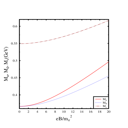
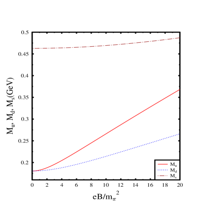
Fig. 1-a	Fig.1-b

Figure 1: Constituent quark masses as functions of magnetic field at zero temperature and zero density. Fig. 1(a) shows the constituent quark masses as a function of the magnetic field when the determinant interaction is taken into account. Fig 1(b) shows the same when the determinant interaction term is ignored i.e. $K=0$. The solid curves refer to constituent masses of u- quark, the dotted curve refers to the constituent mass of the d-quarks while the dot-dashed curve refers to the same of the strange quark.

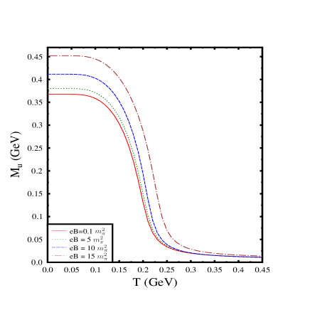
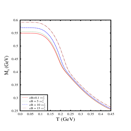
Fig. 2-a	Fig.2-b

Figure 2: Constituent quark masses when charge neutrality conditions are not imposed. Fig.2-a shows the $M_{u}$ at zero baryon chemical potential as a function of temperature for different values of the magnetic field. Fig. 2-b shows the same for the strange quark mass $M_{s}$. Both the subplots correspond to nonzero values for the current quark masses given as $m_{u}$=5.5 MeV and $m_{s}$=140.7 MeV.

Let us begin the discussion of the results for the case when the charge neutrality condition is not imposed. In this case $\mu_{e}=0$ and all the quark flavors have the same chemical potential $\mu_{q}$. For given values of $\mu_{q}$, $T(=\beta^{-1})$ and $eB$, we solve the mass gap equation Eq.(41) self consistently using the expression Eq.(46) for the order parameter. Few comments regarding the evaluation of $I^{i}_{med}$ of Eq.(46) may be worth mentioning. In these evaluations, while considering zero temperature and nonzero $\mu_{q}$, the Landau levels are filled up upto a maximum value of $n$, $n_{max}={\rm Int}\left[\frac{\Lambda^{2}}{2|q_{i}|B}\right]$ as already mentioned in the previous section. On the other hand, for all finite temperature calculations, the levels are filled upto the maximum Landau level, so that the error in neglecting the higher Landau level is less than $10^{-5}$. We also observe that for low temperatures, near the cross over transition temperature, there could be multiple solutions of the mass gap equation corresponding to multiple extrema of the thermodynamic potential. In such cases, we have chosen the solution which has the least value of the thermodynamic potential given in Eq.(48). We ensure this by verifying the positivity of the second derivative of the thermodynamic potential with respect to the corresponding masses.

We show the constituent masses of the three flavors of quarks as modified by magnetic field at zero temperature and zero density in Fig.1. The magnetic field enhances the order parameters as reflected in the values of the constituent masses $M_{u}$, $M_{d}$ and $M_{s}$. Because of charge difference, this enhancement is not the same for all the quarks. For the couplings $G$ and $K$ as chosen here, the enhancement factors $(M(B)-M(B=0))/M(B=0)$ e.g. for $eB=20m_{\pi}^{2}$ are about 35$\%$, 24$\%$, 12$\%$ for u,d and s quarks respectively. We might mention here that the effect of magnetic field on chiral symmetry breaking has been considered in NJL model in Ref.klimenkoplb without the KMT determinant interaction term. For a comparison, we have also plotted in Fig. 1 b, the constituent quark masses without the determinant term as a function of the magnetic field. Clearly, the mass splitting between $u$ and $d$ quarks is much larger when the determinant interaction is not taken in to account– e.g.$(M_{u}(B)-M_{d}(B))/M_{u}(B=0)=57\%$ at $eB=20m_{\pi}^{2}$ when K=0 while the same ratio is about $11\%$ when $K\Lambda^{5}=12.36$. This behavior can be understood as follows. Whereas the magnetic field tends to differentiate the constituent quark masses of different flavors, the determinant interaction which causes mixing between the constituent quarks of different flavors tends to bring the constituent quark masses together. This results in the splitting between the constituent quarks of different flavors becoming smaller when determinant interaction is included in presence of magnetic field. Such a behavior is also observed in Ref.boomsma for the case of two flavor NJL model.

We then show the temperature dependence of the constituent quark masses of the u and s quark for zero chemical potential for different strengths of the magnetic field, in Fig.2. The phase transition remains a smooth crossover as is the case with zero magnetic field. The effect of magnetic field as a catalyser of chiral symmetry breaking is also evident. The chiral condensate and hence the constituent quark masses increase in the temperature regime considered here when the magnetic field is increased. In these calculations all the Landau levels as appropriate for the given magnetic field have been filled up and the lowest Landau level approximation has not been assumed. The qualitative aspects of the phase transition remains the same as in case of zero magnetic field. This result is in contrast to the linear sigma model coupled to quarks fraga where the usual cross over becomes a first order phase transition in the presence of strong magnetic field. We might mention here that our results are similar to that of Ref.boomsma for the two flavor NJL model.

Next, we discuss the behavior of constituent masses as baryon number density is increased at zero temperature and for different strengths of magnetic field. In Fig.3, we show the dependence of the constituent masses $M_{u}$, $M_{d}$ and $M_{s}$ on the quark chemical potential at zero temperature for three different strengths of magnetic field. For zero magnetic field, as the quark chemical potential is increased, a first order transition is observed to take place for the value of $\mu_{q}=\mu_{c}\sim 0.362$GeV. At lower values of the quark chemical potential ($\mu_{q}<\mu_{c})$, the masses of the quarks stay at their vacuum values and the baryon number density remains zero. At $\mu=\mu_{c}$, the first order transition takes place and the light quarks have a drop in their masses from their vacuum values of about 367 MeV to about 52 MeV. The baryon number density also jumps from zero to $2.37\rho_{0}$, with $\rho_{0}=0.17{\rm fm}^{-3}$ being the normal nuclear matter density. Because of the six fermion KMT term, this first order transition for the light quarks is also reflected in dropping of the strange quark mass from its vacuum value of 549 MeV to about 464 MeV.

As the magnetic field is increased, the critical chemical potential for this first order transition consistently decreases as may be clear from figures Fig. 3a, Fig 3b and Fig 3c. For $eB=10m_{\pi}^{2}$,$eB=15m_{\pi}^{2}$, the corresponding values of $\mu_{c}$ are 0.327 GeV and 0.323 GeV respectively. For $\mu<\mu_{c}$, the constituent quark masses increases with the magnetic field as may be seen in Fig. 3a where we have plotted the d-quark mass as a function of quark chemical potential. E.g. for $eB=10m_{\pi}^{2}$, the increase in masses of the u and d quarks are about 45 MeV and 30 MeV respectively while for strange quarks the corresponding increase in mass is about 21 MeV as compared to zero field case. Since the $\mu_{c}$ decreases with increase in magnetic field, there are windows in the range of chemical potential where it appears e.g. in Fig 3a for the u-quark, that the mass decreases with the magnetic field in the range of chemical potential between $\mu=323$ MeV to $\mu=362$ MeV. In this regime however, the chiral transition already has taken place for $eB=15m_{\pi}^{2}$. For $eB=10m_{\pi}^{2}$, in this regime of chemical potential although the first order transition takes place, the transition is weaker compared to the case of $eB=15m_{\pi}^{2}$ in the sense that the constituent quark mass is higher compared to the case of $eB=15m_{\pi}^{2}$. Finally, for the case of zero magnetic field, the transition is still to take place. After the transition the ordering in the masses changes depending upon the filling up of the Landau levels in case of nonzero magnetic fields. The kinks in the mass variation correspond to filling up of the Landau levels. This decrease of critical chemical potential due to the presence of magnetic field has also been observed in dense holographic matter and is termed as inverse magnetic catalysis of chiral symmetry breaking andreasrebhan . We, however, observe that although the critical chemical potential decreases with magnetic field, the corresponding baryonic density increases. This is clearly seen in Fig. 4 where we have shown the baryon number density as a function of quark chemical potential for different strengths of magnetic field. While for $eB=10m_{\pi}^{2}$, the critical density $\rho_{c}/\rho_{0}=2.39$ is almost similar to the zero field value of the same $\rho_{c}/\rho_{0}=2.38$, the critical density for $eB=15m_{\pi}^{2}$ is substantially larger with $\rho_{c}/\rho_{0}=3.62$. Similar qualitative behavior was also observed in Ref.providencia .

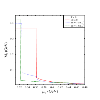
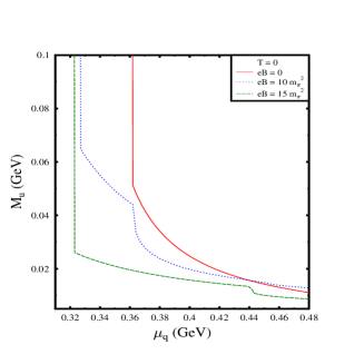
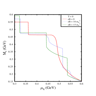
Fig. 3-a	Fig.3-b	Fig.3-c

Figure 3: Constituent quark masses as functions of $\mu_{q}$ at $T=0$ for different strength of magnetic field. Constituent quark masses of d,u and s quarks are plotted in Fig a, Fig b and Fig c respectively.

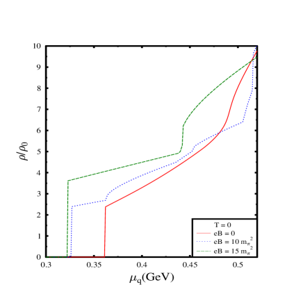
Figure 4: Baryon density as a function of quark chemical potential for different strengths of magnetic field.

At finite chemical potential, we also observe oscillations of the order parameter with the magnetic field as shown in Fig.5 for u-quark. We have taken the value of the chemical potential as $\mu_{q}=380$ MeV and taken the temperature, T as zero. This phenomenon is similar to the oscillation of the magnetization of a material in presence of external magnetic field, known as de Hass van Alphen effect ebertmag . As observed earlier, this is a consequence of oscillations in the density of states at Fermi surface due to the Landau quantization. The oscillatory behavior is seen as long as $2|q|B<\sqrt{\mu_{q}^{2}-M_{q}^{2}}$ and ceases when the first Landau level lies above the Fermi surface fukuwarringa ; noornah .

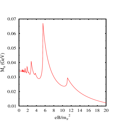
Figure 5: Oscillation of u-quark mass with magnetic field. We have taken $\mu_{q}=380$ MeV and T=0.

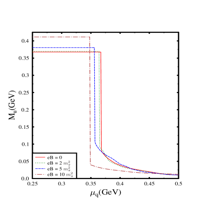
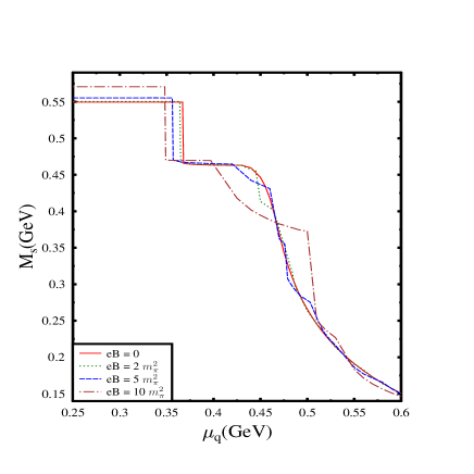
Fig. 6-a	Fig.6-b

Figure 6: Constituent quark masses for charge neutral matter. Masses of up quarks (a) and strange quarks (b) as functions of the quark chemical potential, $\mu_{q}$ at T=0 for different strengths of magnetic field

We then discuss the effects of magnetic field on charge neutral dense matter as may be relevant for the matter in the interior of the neutron stars. The thermodynamic potential is numerically computed as follows. For given values of the quark chemical potential $\mu_{q}$, the electric charge chemical potential $\mu_{E}$ and magnetic field $eB$, the coupled mass gap equations given by Eq.(41) are solved, using the expression Eq.(46) for the order parameter. The values of the electric charge chemical potential $\mu_{E}$ are varied so that the charge neutrality condition Eq. (57) is satisfied. The resulting solutions are then used in Eq.(48) to compute the thermodynamic potential. In doing so, we also check if there are multiple solutions to the gap equation and choose the one that has the least value of the thermodynamic potential. In Fig. 6, we show the masses of the quarks as functions of chemical potential for charge neutral matter for zero temperature. Let us note that at the transition point, the d-quark number density is almost twice that of u-quark number density to maintain charge neutrality as mass of s-quark is much too large to contribute to the charge density. For this to be realized, the mass of d-quark should be sufficiently smaller as compared the mass of u quark to generate the required difference in the number densities. This, in turn, means that $\mu_{d}$ should be larger than $\mu_{u}$ unlike the charge neutral case where all the quarks have the same chemical potential. Numerically, it turns out that for zero magnetic field this condition is satisfied when $\mu_{d}\sim 393$ MeV and $\mu_{u}\sim 318$ MeV as compared to the common chemical potential $\mu_{c}=362$ MeV when charge neutrality condition is not imposed. The corresponding masses of d and u quarks are about $61{\rm MeV}$ and $80{\rm MeV}$ respectively compared to the common mass of $52{\rm MeV}$ at the critical chemical potential when charge neutrality is not imposed. These values of $\mu_{u}$ and $\mu_{d}$ at the transition point corresponds to a electron chemical potential of $\mu_{e}\sim 75$ MeV at the transition while the corresponding quark chemical potential at the transition is $\mu_{q}=368{\rm MeV}\equiv\mu_{c}$, which is slightly higher as compared to the value of $\mu_{c}=362{\rm MeV}$ for the case when such neutrality condition is not imposed. At the transition point for the neutral matter, the number density of d quarks is almost twice that of u quarks while the electron number density is three orders of magnitude lower than either of the quark number densities. As the magnetic field is increased, the constituent masses for the three quarks increase for chemical potential smaller than the critical chemical potential. The first sudden drop of the strange quark mass (see Fig.6b) is related to the drop in the light quark masses through the determinant interaction. The kink structure in the strange quark mass for higher magnetic fields can be identifiable with the filling of different Landau levels. Further, it is observed that a higher magnetic field leads to a smaller value for $\mu_{c}$. Similar to the case of non charge neutral matter, however, the critical density becomes higher for increased magnetic field. This magnetic catalysis of chiral symmetry breaking is clearly shown in Fig.7, where masses of up and strange quarks are shown as functions of baryon density for zero temperature and for different strengths of magnetic field.

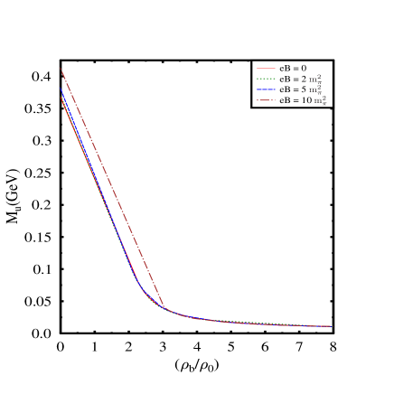
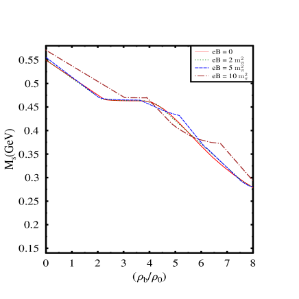
Fig. 7-a	Fig.7-b

Figure 7: Constituent quark masses of u and s quark masses as functions of baryon density in units of nuclear matter density $\rho_{0}$ for different strengths of magnetic field at T=0.

We then study the effect of magnetic field on the equation of state, i.e. pressure as a function of energy for the charge neutral matter. This is shown in Fig. 8 for zero temperature. The effect of Landau quantization shows up in the kink structure of the equation of state. For smaller magnetic fields, this effect is less visible as the number of filled Landau levels are quite large. Further, it may be observed that as the magnetic field is increased, the equation of state becomes somewhat stiffer. Since the zero density constituent quark masses increase with magnetic field, the vacuum energy density becomes lower compared to the zero field case. Therefore the starting values of pressure in presence of field becomes higher compared to the zero field case as seen in Fig.8. For higher densities when chiral symmetry is restored, let us first note that the contribution to the thermodynamic potential due to the magnetic field as given in Eq.(50) increases with magnetic field. Therefore, it means that one has to have a larger chemical potential for lower magnetic field as compared to higher field to have the same energy density. So one would naively expect the pressure ($P=\mu\rho-\epsilon$) with lower field to be higher. However, one has to note that chiral symmetry is restored at a lower chemical potential for higher magnetic field as may be clear from Fig.6 and hence the number densities can become higher leading to a higher pressure. This is what actually happens for larger energy densities for the two fields shown in Fig.8. Because of the lower critical chemical potential for the case of $eB=10m_{\pi}^{2}$, the masses of the quarks are smaller and hence the densities becomes higher compared to the case of $eB=5m_{\pi}^{2}$ for the same energy densities leading to a stiffer equation of state.

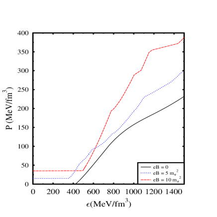
Figure 8: Equations of state for charge neutral matter at zero temperature for different strengths of the magnetic field.

Next, we discuss the effects of magnetic field on hot neutral quark matter. Such a condition is relevant for the matter in the interior of the proto neutron stars where the temperatures could be of about few tens of MeV. In Fig.8, we show the effect of temperature on the masses of the quarks in the magnetized neutral matter. As may be expected, the effect of temperature smoothes the behavior of the masses as functions of the quark chemical potential. The corresponding equations of state are also shown in Fig.9.

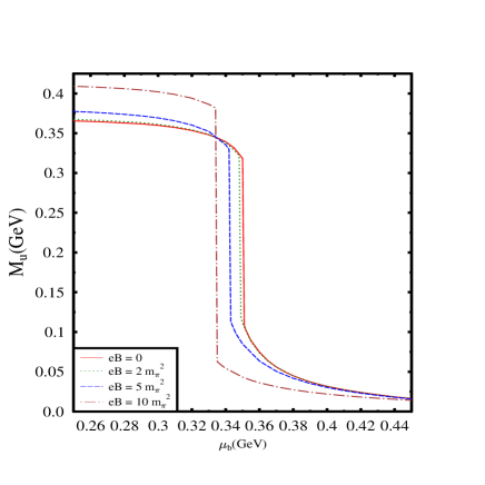
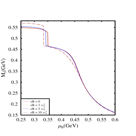
Fig. 9-a	Fig.9-b

Figure 9: Constituent masses of u and s quarks as functions of $\mu_{q}$ for charge neutral matter for different strengths of magnetic field at T=40 MeV

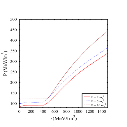
Figure 10: Equation of state for charge neutral matter at T=40 MeV for different magnetic field.

Let us note that in the equation of state that we have plotted in Fig.8 and Fig.10, the pressure here corresponds to the thermodynamic pressure i.e. negative of the thermodynamic potential given in Eq.(48). However, in presence of magnetic field, the hydrodynamic pressure can be highly anisotropic canuto ; armendirk ; ferrer3 when there is significant magnetization of the matter. The pressure in the direction of the field $P_{\parallel}$ is the thermodynamic pressure $P=-\Omega$ as defined in Eq.(48). On the other hand, the pressure $P_{\perp}$ in the transverse direction of the applied magnetic field is given by $P_{\perp}=P-MB$ armendirk . Here, $M=-\partial\Omega/\partial B$ is the magnetization of the system. Using the thermodynamic potential expression given in Eq.(48), this can be written as

$$M=M_{med}+M_{field}+M_{c}$$ (60)

where, $M_{med}$ , the contribution the magnetization from the medium which at zero temperature is given by

$$M_{med}=-\frac{\partial\Omega_{med}}{\partial B}=\frac{N_{c}}{4\pi^{2}}\sum_{n,i}\alpha_{n}|q_{i}|\left[\mu_{i}p_{zmax}^{i}-(A_{n}^{2}+2n|q_{i}|B)\log\frac{\mu_{i}+p_{zmax}^{i}}{A_{n}}\right]$$ (61)

where, we have abbreviated $A_{n}=\sqrt{M^{2}+2n|q_{i}|B}$. $M_{field}$ is the contribution from the field part of the thermodynamic potential $\Omega_{field}$ given as

$$M_{field}=-\frac{\partial\Omega_{field}}{\partial B}=\sum_{i}q_{i}^{2}B\left[\frac{\log x_{i}}{12}-\frac{1}{24}+x_{i}^{3}I_{1}(x_{i})\right],$$ (62)

where,

$$I_{1}(x)=\frac{1}{\pi}\int y\frac{2\arctan(y)+y\log(1+y^{2})}{(\exp(2\pi xy)-1)(1-\exp(-2\pi y)}dy$$ (63)

We might note here that $\Omega_{field}$ term originates from the effect of magnetic field on the Dirac sea so that we can recognize that $M_{field}$ is due the magnetization of the Dirac sea.

Finally, $M_{c}$ in Eq.(60) is the contribution to the magnetization arising from the last two terms of the thermodynamic potential in Eq.(48) and is given as

$$M_{c}=-4G\sum_{i}I_{i}\frac{\partial I_{i}}{\partial B}-2K\sum_{i\neq j\neq k}I_{i}I_{j}\frac{\partial I_{k}}{\partial B}.$$ (64)

Here, $\frac{\partial I_{i}}{\partial B}$ is the derivative of the quark condensate (-$\langle\bar{\psi}_{i}\psi\rangle$) with respect to the magnetic field given as

$$\frac{\partial I_{i}}{\partial B}=\frac{\partial I_{med}^{i}}{\partial B}+\frac{\partial I_{field}^{i}}{\partial B},$$

where, the contribution from the medium at zero temperature is

$$\frac{\partial I_{med}^{i}}{\partial B}=\sum_{n}\frac{N_{c}\alpha_{n}}{2\pi^{2}}\left[\log\frac{p_{zmax}^{i}+\mu_{i}}{A_{n}}-\frac{n|q_{i}|B}{A_{n}^{2}}\frac{\mu_{i}}{p_{zmax}^{i}}\right],$$ (65)

and, the field contribution from the condensate to magnetization

$$\frac{\partial I_{field}^{i}}{\partial B}=\frac{N_{c}}{2\pi^{2}}\left[\log\Gamma(x_{i})+\frac{1}{2}\log\frac{x_{i}}{2\pi}+x_{i}-x_{i}\Psi^{0}(x_{i})-\frac{1}{2}\right],$$ (66)

where, as defined earlier $x_{i}=(M_{i}^{2}/2|q_{i}|B)$ and $\Psi^{0}(x)=\frac{\Gamma^{\prime}(x)}{\Gamma(x)}$ is the logarithmic derivative of the Gamma function.

The resulting magnetization at T=0 is plotted in Fig.11 for $\mu_{u}=0.4GeV=\mu_{d}$. The magnetization exhibits rapid de Hass-van Alphen oscillations. The irregularity in the oscillation is due to the unequal masses of the three quarks which are calculated self consistently using the gap equation. Unlike in Ref.armendirk , the magnetization does not become constant even after the all the quarks are in the lowest Landau level. This is due to the effect of contribution of magnetization from the Dirac sea which is included here along with the Fermi sea contribution given by $M_{medium}$.

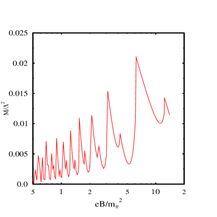
Figure 11: Magnetization in units of $\Lambda^{2}$ as a function of magnetic field. The magnetic field in units of $m_{\pi}^{2}$ is plotted in a logarithmic scale. We have taken here T=0 and $\mu_{u}=0.4GeV=\mu_{d}$.

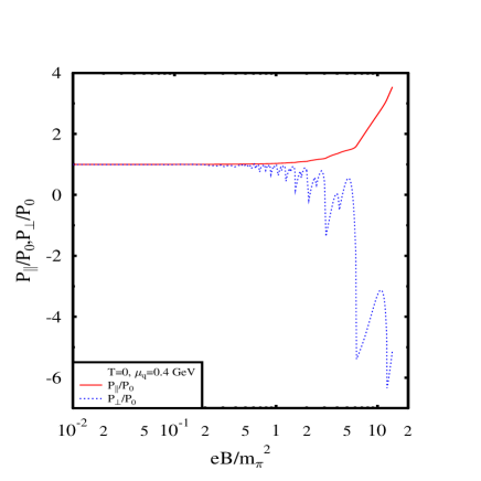
Figure 12: The parallel $P_{\parallel}$ and transverse $P_{\perp}$ pressures of strange quark matter as functions of the magnetic field in units of pressure $P_{0}$ for zero magnetic field. Magnetic field in units of $m_{\pi}^{2}$ is plotted in a logarithmic scale. We have taken here T=0 and $\mu_{u}=0.4GeV=\mu_{d}$.

The transverse and the longitudinal pressure for the system is plotted in Fig.12. Here, we have taken T=0 and $\mu=400$MeV. The oscillatory behavior of the magnetization is reflected in the transverse pressure. The two pressures start to differ significantly for magnetic field strengths of about $eB=m_{\pi}^{2}$ which corresponds to about $10^{18}$ Gauss. Such field induced anisotropy in pressure is qualitatively similar as in Ref. armendirk , where, the anisotropic properties of transport coefficients for strange quark matter were considered. While considering neutron star structure, one has to also include the free field energy $\frac{1}{2}B^{2}$ to the total energy and pressure. This term adds to the parallel and the transverse pressure with different signs ferrer3 . This can make the pressure in the transverse direction negative leading to mechanical instability ferrer3 . While studying structural properties of compact astrophysical objects endowed with magnetic fields such splitting of the pressure in to the parallel and perpendicular direction need to be taken into account as this can effect the structure and geometry of the star.

Finally we end this section with a comment regarding the axial fermion current density induced at finite chemical potential. From Eq.s(31) and Eq.(42),

$$\langle j_{5}^{i3}\rangle=\frac{N_{c}|q_{i}|B}{(2\pi)^{2}}\int{dp_{z}\bigg{[}\frac{1}{\exp(\sqrt{p_{z}^{2}+M_{i}^{2}}-\mu_{i})}-\frac{1}{\exp(\sqrt{p_{z}^{2}+M_{i}^{2}}+\mu_{i})}}\bigg{]}.$$ (67)

Thus, although the lowest Landau level contributes to the above expectation value, because of its dependence on the constituent quark mass parameter $M_{i}$, the effects of all the higher Landau levels are implicitly there in Eq.(67) as the constituent masses here are calculated self consistently using Eq.(41) and Eq.(46). Further, because of dependence on the constituent quark mass the axial quark current density expectation value also depends upon the coupling in a nonperturbative manner igormag ; hongmag .

V summary

We have analyzed here the ground state structure for chiral symmetry breaking in presence of strong magnetic field. The methodology uses an explicit variational construct for the ground state in terms of quark-antiquark pairing. A nice feature of the approach is that the four component quark field operator in presence of magnetic field could get expressed in terms of the ansatz functions that occurs for the description of the ground state. Apart from the methodology being new, we also have new results. Namely, the present investigations have been done in a three flavor NJL model along with a flavor mixing six quark determinant interaction at finite temperature and density and fields within the same framework. In that sense it generalizes the two flavor NJL model considered in Ref.boomsma for both finite temperature and density. The gap functions and the thermal distribution functions could be determined self consistently for given values of the temperature, the quark chemical potential and the strength of magnetic field. At zero baryon density and high temperature, the qualitative feature of chiral transition remains a cross over transition even for magnetic field strength eB=10m${}_{\pi}^{2}$. The magnetic catalysis of chiral symmetry breaking is also observed.

At finite densities, the effects of Landau quantization is more dramatic. The order parameter shows oscillation similar to the de Hass van Alphen effect for magnetization in metals. However, in the present case of dense quark matter, the mass of the quark itself is dependant on the strength of magnetic fields which leads to a non periodic oscillation of the order parameter. Although the critical chemical potential, $\mu_{c}$, for chiral transition consistently decreases with increase in the strength of the magnetic field, the corresponding density increases with the magnetic field strength. Imposition of electrical charge neutrality condition for the quark matter increases the value for $\mu_{c}$. Since the mass of the strange quark plays an important role in maintaining the charge neutrality condition, this in turn affects the chiral restoration transition in quark matter. The presence of nonzero magnetic field appears to make the equation of state stiffer. Further, the pressure could be anisotropic if the magnetization of the matter is significant. Within the model, this anisotropy starts to become relevant for field strengths around $10^{18}$ Gauss. While considering the structural properties of astro physical compact objects having magnetic fields this anisotropy in the equation of state should be taken into account as it can affect the geometry and structure of the star.

We have considered here quark-antiquark pairing in our ansatz for the ground state which is homogeneous with zero total momentum as in Eq.(7). However, it is possible that the condensate could be spatially non-homogeneous with a net total momentum dune ; frolov ; nickel . Further, one could include the effect of deconfinement transition by generalizing the present model to Polyakov loop NJL models for three flavors to investigate the inter relationship of deconfinement and the chiral transition in presence of strong fields for the three flavor case considered heregato . This will be particularly important for finite temperature calculations. At finite density and small temperatures, the ansatz can be generalized to include the diquark condensates in presence of magnetic field digal ; iran ; ferrerscmag . Some of these calculations are in progress and will be reported elsewhere.

Appendix A Spinors in a constant magnetic field

Here we derive the solutions for the spinors for a relativistic charged particle in presence of an external constant magnetic field and the field operator expansion for the corresponding fermion field. We shall take the direction of the magnetic field to be in the z-direction. We choose the corresponding gauge field $A_{\mu}=(0,0,Bx,0)$. The Dirac equation in presence of the uniform magnetic field is then written as

$$i\frac{\partial\psi}{\partial t}=(\mathchoice{\mbox{\boldmath$\alpha$}}{\mbox{\boldmath$\alpha$}}{\mbox{\boldmath$\scriptstyle\alpha$}}{\mbox{\boldmath$\scriptscriptstyle\alpha$}}\cdot\mathchoice{\mbox{\boldmath$\Pi$}}{\mbox{\boldmath$\Pi$}}{\mbox{\boldmath$\scriptstyle\Pi$}}{\mbox{\boldmath$\scriptscriptstyle\Pi$}}+\beta m)\psi,$$ (68)

where, $\mathchoice{\mbox{\boldmath$\Pi$}}{\mbox{\boldmath$\Pi$}}{\mbox{\boldmath$\scriptstyle\Pi$}}{\mbox{\boldmath$\scriptscriptstyle\Pi$}}={\bf{p}}-q{\bf{A}}$ is the kinetic momentum of the particle with electric charge $q$ in the presence of the magnetic field.

Let us first derive the positive energy solutions $U(x)$ of Eq.(68). For stationary solution of energy $E$ we choose $U(x)$ as

$$U({\bf{x}},t)=\left[\begin{array}[]{c}\phi({\bf{x}})\\ \chi({\bf{x}})\\ \end{array}\right]e^{-iEt},$$ (69)

where $\phi({\bf{x}})$ and $\chi({\bf{x}})$ are the two component spinors. Substitution this ansatz in Eq.(68) leads to

$$\chi(\mathchoice{\mbox{\boldmath$x$}}{\mbox{\boldmath$x$}}{\mbox{\boldmath$\scriptstyle x$}}{\mbox{\boldmath$\scriptscriptstyle x$}})=\frac{\mathchoice{\mbox{\boldmath$\sigma$}}{\mbox{\boldmath$\sigma$}}{\mbox{\boldmath$\scriptstyle\sigma$}}{\mbox{\boldmath$\scriptscriptstyle\sigma$}}\cdot\mathchoice{\mbox{\boldmath$\Pi$}}{\mbox{\boldmath$\Pi$}}{\mbox{\boldmath$\scriptstyle\Pi$}}{\mbox{\boldmath$\scriptscriptstyle\Pi$}}}{E+m}\phi(\mathchoice{\mbox{\boldmath$x$}}{\mbox{\boldmath$x$}}{\mbox{\boldmath$\scriptstyle x$}}{\mbox{\boldmath$\scriptscriptstyle x$}}),$$ (70)

so that eliminating $\chi$ in favor of $\phi$, leads to an equation for the latter as

$$(E^{2}-m^{2})\phi(\mathchoice{\mbox{\boldmath$x$}}{\mbox{\boldmath$x$}}{\mbox{\boldmath$\scriptstyle x$}}{\mbox{\boldmath$\scriptscriptstyle x$}})=(\mathchoice{\mbox{\boldmath$\sigma$}}{\mbox{\boldmath$\sigma$}}{\mbox{\boldmath$\scriptstyle\sigma$}}{\mbox{\boldmath$\scriptscriptstyle\sigma$}}\cdot\mathchoice{\mbox{\boldmath$\Pi$}}{\mbox{\boldmath$\Pi$}}{\mbox{\boldmath$\scriptstyle\Pi$}}{\mbox{\boldmath$\scriptscriptstyle\Pi$}})^{2}\phi(\mathchoice{\mbox{\boldmath$x$}}{\mbox{\boldmath$x$}}{\mbox{\boldmath$\scriptstyle x$}}{\mbox{\boldmath$\scriptscriptstyle x$}}).$$ (71)

Noting that $({\bf{\sigma}}\cdot{\bf{\Pi}})^{2}={\bf{\Pi}}^{2}-q{\bf{\sigma}}\cdot{\bf{B}}$. With ${\bf{B}}=(0,0,B)$ and with our choice of the gauge $A_{\mu}=(0,0,Bx,0)$, the above equation reduces to

$$(E^{2}-m^{2})\phi({\bf{x}})=[-\nabla^{2}+(qBx)^{2}-qB(\sigma_{3}+2xp_{y})]\phi({\bf{x}})$$ (72)

Next, recognizing the fact that in the RHS, the coordinates $y$ and $z$ do not occur explicitly except for in the derivatives, we might assume the solution to be of the form

$$\phi({\bf{x}})=e^{i(p_{y}y+p_{z}z)}f(x)$$ (73)

where, $f(x)=f_{\alpha}u_{\alpha}$, $\alpha=\pm 1$ for spin up and spin down respectively with $u_{1}=\left(\begin{array}[]{c}1\\ 0\\ \end{array}\right)$; $u_{-1}=\left(\begin{array}[]{c}0\\ 1\\ \end{array}\right)$; so that $\sigma_{3}f=\alpha f$. Using Eq.(73) in Eq.(72) we have,

$$\left[\frac{\partial^{2}}{\partial\xi^{2}}-\xi^{2}+a_{\alpha}\right]f_{\alpha}(\xi)=0,$$ (74)

where, we have introduced the dimensionless variables $\xi=\sqrt{|q|B}\left(x-\frac{p_{y}}{qB}\right)$ and $a_{\alpha}=\frac{E^{2}-m^{2}-p_{z}^{2}+qB\alpha}{|q|B}$. Eq.(74) is a special form of Hermite differential equation, whose solutions exist for $a_{\alpha}=2n+1$, $n=0,1,2,...$. This gives the energy levels as

$$E_{n\alpha}^{2}=m^{2}+p_{z}^{2}+(2n+1)|q|B-qB\alpha.$$ (75)

The solution of Eq.(74) is

$$f_{\alpha}(\xi)=c_{n}e^{-\frac{\xi^{2}}{2}}H_{n}(\xi)=I_{n}(\xi),$$ (76)

Where $H_{n}(\xi)$ is the Hermite polynomial of the nth order, with the normalization constant $c_{n}$ given by

$$c_{n}=\sqrt{\frac{\sqrt{|q|B}}{n!2^{n}\sqrt{\pi}}}.$$

The functions $I_{n}(\xi)$’s satisfy the completeness relation

$$\sum_{n}I_{n}(\xi)I_{n}(\xi`)=|q|B\delta(\xi-\xi^{\prime}).$$ (77)

Further using orthonormality condition for the Hermite polynomials, $I_{n}$’s are normalized as

$$\int d\xi I_{n}(\xi)I_{m}(\xi)=\sqrt{|q|B}\delta_{n,m},$$ (78)

$I_{n}(\xi)$’s are seen to satisfy the following relations

$$\frac{\partial}{\partial x}I_{n}(\xi)=\sqrt{|q|B}[-\xi I_{n}(\xi)+\sqrt{2n}I_{n-1}(\xi)]$$ (79)

$$2\xi I_{n}(\xi)=\sqrt{2n}I_{n-1}(\xi)+\sqrt{2(n+1)}I_{n+1}(\xi)$$ (80)

Thus with the upper component $\phi({\bf{x}})$ known from Eq.(73) and Eq.(76), the lower component $\chi({\bf{x}})$ can be evaluated from Eq.(70) using the relations Eq.(80). This leads to the explicit solutions for the positive energy spinors as $U({\bf{x}},t)=U(n,{\bf{p}}_{{}_{\!\hbox to0.0pt{$\scriptscriptstyle\backslash$\hss}{\scriptscriptstyle x}}},x)\exp(i{\bf{p}}_{{}_{\!\hbox to0.0pt{$\scriptscriptstyle\backslash$\hss}{\scriptscriptstyle x}}}\cdot{\bf{x}}_{{}_{\!\hbox to0.0pt{$\scriptscriptstyle\backslash$\hss}{\scriptscriptstyle x}}}-i\epsilon_{n}t)$ with

$$U_{\uparrow}(x,\mathchoice{\mbox{\boldmath$p$}}{\mbox{\boldmath$p$}}{\mbox{\boldmath$\scriptstyle p$}}{\mbox{\boldmath$\scriptscriptstyle p$}}_{{}_{\!\hbox to0.0pt{$\scriptscriptstyle\backslash$\hss}{\scriptscriptstyle x}}},n) = \frac{1}{\sqrt{2\epsilon_{n}(\epsilon_{n}+m)}}\left(\begin{array}[]{c}(\epsilon_{n}+m)\left(\Theta(q)I_{n}+\Theta(-q)I_{n-1}\right)\\ 0\\ p_{z}\left(\Theta(q)I_{n}+\Theta(-q)I_{n-1}\right)\\ -i\sqrt{2n|q|B}\left(\Theta(q)I_{n-1}+\Theta(-q)I_{n}\right)\\ \end{array}\right)$$ (81e)

$$U_{\downarrow}(x,\mathchoice{\mbox{\boldmath$p$}}{\mbox{\boldmath$p$}}{\mbox{\boldmath$\scriptstyle p$}}{\mbox{\boldmath$\scriptscriptstyle p$}}_{{}_{\!\hbox to0.0pt{$\scriptscriptstyle\backslash$\hss}{\scriptscriptstyle x}}},n) = \frac{1}{\sqrt{2\epsilon_{n}(\epsilon_{n}+m)}}\left(\begin{array}[]{c}0\\ (\epsilon_{n}+m)\left(\Theta(q)I_{n-1}+\Theta(-q)I_{n}\right)\\ i\sqrt{2n|q|B}\left(\Theta(q)I_{n}-\Theta(-q)I_{n-1}\right)\\ -p_{z}\left(\Theta(q)I_{n}-\Theta(-q)I_{n-1}\right)\\ \end{array}\right).$$ (81j)

In the above, we have defined $\epsilon_{n}=\sqrt{p_{z}^{2}+m^{2}+2n|q|B}$ and further, we have defined $I_{-1}=0$ while for nonnegative values of $n$, $I_{n}(\xi)$’s are given by Eq.(76).

In an identical manner, one can obtain the solutions for the antiparticles and the solution can be written as $V({\bf{x}},t)=V(x,{\bf{p}}_{{}_{\!\hbox to0.0pt{$\scriptscriptstyle\backslash$\hss}{\scriptscriptstyle x}}},n)exp(-i{\bf{p}}_{{}_{\!\hbox to0.0pt{$\scriptscriptstyle\backslash$\hss}{\scriptscriptstyle x}}}\cdot{\bf{x}}_{{}_{\!\hbox to0.0pt{$\scriptscriptstyle\backslash$\hss}{\scriptscriptstyle x}}}+i\epsilon_{n}t)$ with

$$V_{\uparrow}(x,-{\bf{p}}_{{}_{\!\hbox to0.0pt{$\scriptscriptstyle\backslash$\hss}{\scriptscriptstyle x}}},n) = \frac{1}{\sqrt{2\epsilon_{n}(\epsilon_{n}+m)}}\left(\begin{array}[]{c}\sqrt{2n|q|B}\left(\Theta(q)I_{n}-\Theta(-q)I_{n-1}\right)\\ ip_{z}\left(\Theta(q)I_{n-1}+\Theta(-q)I_{n}\right)\\ 0\\ i(\epsilon_{n}+m)\left(\Theta(q)I_{n-1}+\Theta(-q)I_{n}\right)\\ \end{array}\right),$$ (82e)

$$V_{\downarrow}(x,-\mathchoice{\mbox{\boldmath$p$}}{\mbox{\boldmath$p$}}{\mbox{\boldmath$\scriptstyle p$}}{\mbox{\boldmath$\scriptscriptstyle p$}}_{{}_{\!\hbox to0.0pt{$\scriptscriptstyle\backslash$\hss}{\scriptscriptstyle x}}},n) = \frac{1}{\sqrt{2\epsilon_{n}(\epsilon_{n}+m)}}\left[\begin{array}[]{c}ip_{z}\left(\Theta(q)I_{n}+\Theta(-q)I_{n-1}\right)\\ \sqrt{2n|q|B}\left(\Theta(q)I_{n-1}-\Theta(-q)I_{n-1}\right)\\ -i(\epsilon_{n}+m)\left(\Theta(q)I_{n}+\Theta(-q)I_{n-1}\right)\\ 0\\ \end{array}\right).$$ (82j)

The spinors are normalized as

$$\int dxU_{r}(x,{\bf{p}}_{{}_{\!\hbox to0.0pt{$\scriptscriptstyle\backslash$\hss}{\scriptscriptstyle x}}},n)^{\dagger}U_{s}(x,{\bf{p}}_{{}_{\!\hbox to0.0pt{$\scriptscriptstyle\backslash$\hss}{\scriptscriptstyle x}}},m)=\delta_{n,m}\delta_{r,s}=\int dxV_{r}(x,{\bf{p}}_{{}_{\!\hbox to0.0pt{$\scriptscriptstyle\backslash$\hss}{\scriptscriptstyle x}}},n)^{\dagger}V_{s}(x,{\bf{p}}_{{}_{\!\hbox to0.0pt{$\scriptscriptstyle\backslash$\hss}{\scriptscriptstyle x}}},m)$$ (83)

These spinors are used in Eq.(1) for expansion of the field operators in the momentum space.

.

References

• (1) For reviews see K. Rajagopal and F. Wilczek, arXiv:hep-ph/0011333; D.K. Hong, Acta Phys. Polon. B32,1253 (2001); M.G. Alford, Ann. Rev. Nucl. Part. Sci 51, 131 (2001); G. Nardulli, Riv. Nuovo Cim. 25N3, 1 (2002); S. Reddy, Acta Phys Polon.B33, 4101(2002); T. Schaefer arXiv:hep-ph/0304281; D.H. Rischke, Prog. Part. Nucl. Phys. 52, 197 (2004); H.C. Ren, arXiv:hep-ph/0404074; M. Huang, arXiv: hep-ph/0409167; I. Shovkovy, arXiv:nucl-th/0410191.
• (2) D.Kharzeev, L. McLerran and H. Warringa, Nucl. Phys. A803, 227 (2008); K.Fukushima, D. Kharzeev and H. Warringa,Phys. Rev. D 78, 074033 (2008).
• (3) V. Skokov, A. Illarionov and V. Toneev, Int. j. Mod. Phys. A 24, 5925, (2009).
• (4) D. Kharzeev, Ann. of Physics, K. Fukushima, M. Ruggieri and R. Gatto, Phys. Rev. D 81, 114031 (2010).
• (5) M.D’Elia, S. Mukherjee and F. Sanflippo,Phys. Rev. D 82, 051501 (2010).
• (6) A.J. Mizher, M.N. Chenodub and E. Fraga,arXiv:1004.2712[hep-ph].
• (7) K. Fukushima, M. Ruggieri and R. Gatto, Phys. Rev. D 81, 114031 (2010).
• (8) E.V. Gorbar, V.A. Miransky and I. Shovkovy,Phys. Rev. C 80, 032801(R) (2009); ibid, arXiv:1009.1656[hep-ph].
• (9) V.P. Gusynin, V. Miranski and I. Shovkovy,Phys. Rev. Lett. 73, 3499 (1994); Phys. Lett. B 349, 477 (1995); Nucl. Phys. B462, 249 (1996), E.J. Ferrer and V de la Incerra,Phys. Rev. Lett. 102, 050402 (2009); Nucl. Phys. B824, 217 (2010).
• (10) D. Ebert and K.G. Klimenko,Nucl. Phys. A728, 203 (2003)
• (11) J. K. Boomsma and D. Boer, Phys. Rev. D 81, 074005 (2010)
• (12) D. Bandyopadhyaya, S. Chakrabarty and S. Pal, Phys. Rev. Lett. 79, 2176 (1997); S. Chakrabarty, S. Mandal, Phys. Rev. C 75, 015805 (2007)
• (13) R. C. Duncan and C. Thompson, Astrophys. J. 392, L9 (1992).
• (14) C. Thompson and R. C. Duncan, Astrophys. J. 408, 194 (1993).
• (15) C. Thompson and R. C. Duncan, Mon. Not. R. Astron. Soc. 275, 255 (1995).
• (16) C. Thompson and R. C. Duncan, Astrophys. J. 473, 322 (1996).
• (17) C. Y. Cardall, M. Prakash, and J. M. Lattimer, Astrophys. J. 554, 322 (2001).
• (18) A. E. Broderick, M. Prakash, and J. M. Lattimer, Phys. Lett. B 531, 167 (2002).
• (19) D. Lai and S. L. Shapiro, Astrophys. J. 383, 745 (1991).
• (20) E. J. Ferrer, V. Incera and J. P. Keith, I. Portillo and P. Springsteen, Phys. Rev. C 82, 065802 (2010).
• (21) X.G. Huang, M. Huang, D.H. Rischke and A. Sedrakian, Phys. Rev. D 81, 045015 (2010).
• (22) D.P. Menezes, M. Benghi Pinto, S.S. Avancini and C. Providencia ,Phys. Rev. C 80, 065805 (2009); D.P. Menezes, M. Benghi Pinto, S.S. Avancini , A.P. Martinez and C. Providencia, Phys. Rev. C 79, 035807 (2009)
• (23) H. Mishra and S.P. Misra, Phys. Rev. D 48, 5376 (1993).
• (24) H. Mishra and J.C. Parikh, Nucl. Phys. A679, 597 (2001).
• (25) Amruta Mishra and Hiranmaya Mishra, Phys. Rev. D 69, 014014 (2004).
• (26) K. Bhattacharya,arXiv:0705.4275[hep-th]; M. deJ. Aguiano-Galicia, A. Bashir and A. Raya,Phys. Rev. D 76, 127702 (2007).
• (27) A. Mishra and H. Mishra, Phys. Rev. D 71, 074023 (2005).
• (28) A. Mishra and S.P. Misra, Z. Phys. C 58, 325 (1993).
• (29) S. P. Misra, Indian J. Phys. 70A, 355 (1996).
• (30) H. Umezawa, H. Matsumoto and M. Tachiki Thermofield dynamics and condensed states (North Holland, Amsterdam, 1982) ; P.A. Henning, Phys. Rep.253, 235 (1995).
• (31) Amruta Mishra and Hiranmaya Mishra, J. Phys. G 23, 143 (1997).
• (32) T. Mandal, P. Jaikumar and S. Digal, arXiv:0912.1413 [nucl-th] .
• (33) M. A. Metlitsky and A. R. Zhitnitsky,Phys. Rev. D 72, 045011 (2005).
• (34) E.J. Ferrer, V. de la Incera and C. Manuel, Nucl. Phys. B747,88 (2006).
• (35) S.P. Klevansky, Rev. Mod. Phys.64, 649 (1992).
• (36) Michael Buballa, Phys. Rep.407,205, 2005.
• (37) T. Hatsuda and T. Kunihiro, Phys. Rep.247,221, 1994.
• (38) W.V. Liu and F. Wilczek,Phys. Rev. Lett. 90, 047002 (2003),E. Gubankova, W.V. Liu and F. Wilczek, Phys. Rev. Lett. 91, 032001 (2003).
• (39) J. Berges, K. Rajagopal, Nucl. Phys. B538, 215 (1999).
• (40) E. Elizalde, J. Phys. A:Math. Gen. 18,1637 (1985).
• (41) P. Rehberg, S.P. Klevansky and J. Huefner, Phys. Rev. C 53, 410 (1996).
• (42) M. Lutz, S. Klimt and W. Weise, Nucl Phys. A542, 521, 1992.
• (43) S.B. Ruester, V.Werth, M. Buballa, I. Shovkovy, D.H. Rischke, arXiv:nucl-th/0602018; S.B. Ruester, I. Shovkovy, D.H. Rischke, Nucl. Phys. A743, 127 (2004).
• (44) K. Schertler, S. Leupold and J. Schaffner-Bielich, Phys. Rev. C 60, 025801 (()1999).
• (45) K.G. Klimenko and V. Ch. Zhukovsky,Phys. Lett. B 665, 352 (2008).
• (46) F. Preis, A. Rebhan and A. Schmitt, JHEP 1103(2011),033.
• (47) D. Ebert, K.G. Klimenko, M.A. Vdovichenko and A.S. Vshivtsev, Phys. Rev. D 61, 025005 (1999).
• (48) K. Fukushima and H. J. Warringa, Phys. Rev. Lett. 100, 032007 (2008).
• (49) J. Noornah and I. Shovkovy,Phys. Rev. D 76, 105030 (2007).
• (50) V. Canuto and J. Ventura, Fundam. Cosmic Phys.2, 203 (1977).
• (51) Deog Ki Hong, arXiv:1010.3923[hep-th].
• (52) G.Baser, G. Dunne and D. Kharzeev, Phys. Rev. Lett. 104, 232301 (2010).
• (53) I.E. Frolov, V. Ch. Zhukovsky and K.G. Klimenko, Phys. Rev. D 82, 076002 (2010).
• (54) D. Nickel,Phys. Rev. D 80, 074025 (2009).
• (55) R. Gatto and M. Ruggieri, Phys. Rev. D 82, 054027 (2010).
• (56) Sh. Fayazbakhsh and N. Sadhooghi, Phys. Rev. D 82, 045010 (2010).
• (57) E.J. Ferrer, V. de la Incera and C. Manuel, Phys. Rev. Lett. 95, 152002 (2005); E.J. Ferrer and V. de la Incera, Phys. Rev. Lett. 97, 122301 (2006); E.J. Ferrer and V. de la Incera, Phys. Rev. D 76, 114012 (2007).