An analytic approach to perturbations from an initially anisotropic universe

Abstract

We present the analytic forms for the spectra of the cosmological perturbations from an initially anisotropic universe for the high momentum modes in the context of WKB approximations, as the continuation of the work km . We consider the Einstein gravity coupled to a light scalar field. We then assume that the scalar field has the zero velocity initially and then slowly rolls down on the potential toward the origin. In the slow-roll approximations, the Kasner-de Sitter universe with a planar symmetry is a good approximation as the background evolution. Quantization of the perturbations in the adiabatic vacuum, which we call the anisotropic vacuum, is carried out. For non-planar high momentum modes whose comoving momentum component orthogonal to the plane is bigger than the Hubble parameter at the inflationary phase, the WKB approximation is valid for the whole stage of the isotropization. On the other hand, the planar modes whose comoving momentum component orthogonal to the plane is comparable to the Hubble parameter, is amplified during the process of the anisotropic expansion. In the final gravitational wave spectra, we find that there is an asymmetry between the two polarizations of the gravitational wave because the initial mode mixing does not vanish.

I Introduction

Recent measurements by the WMAP satellite komatsu ; wmap5 ; anomaly1 have suggested that the observed map of cosmic microwave background (CMB) anisotropy is almost consistent with the Gaussian and statistically isotropic primordial fluctuations from inflation. issues on a few anomalies in the CMB temperature map on large angular scales found in the recent data have been controversial. The most well-known fact is that there seems to be the suppression of the observed power of CMB anisotropy on angular scales bigger than sixty degrees anomaly1 . There are other observational facts that imply the effect which induces the violation of the rotational invariance. More precisely, the planarity of lower multipole moments, the alignment between the quadrupole ($\ell=2$) and the octopole ($\ell=3$), and the alignment of them with the equinox and the ecliptic plane anomaly2 were announced. There are other observational facts implying the large-scale anisotropy, i.e., odd correlations of $\ell=4\sim 8$ multipoles with $\ell=2,3$ multipoles copi , a very large, possibly non-Gaussian cold spot in 10 degree scale cruz , asymmetry of angular map measured in north and south hemispheres eriksen (see also the recent review review and more recent references therein). It also should be noted that some authors claim that there is no significant evidence for primordial isotropy breaking in five-year WMAP data Picon (see also more recent arguments gawe ). Indeed, to explain the origin of the anomalies, various solutions have been suggested, introducing a nontrivial topology topology , a local anisotropy based on the Bianchi type VII_h universe to explain the quadrupole/octopole planarity and alignment jaffe , non-linear inhomogeneities moffat and assuming an elliptic universe to explain the suppression of the quadrupole CMB power eli . More recently, in particular, models which introduce an explicit source to break the spatial isotropy, either during inflation or in the late time universe, have been proposed, e.g., by the dynamics of an anisotropic energy-momentum component during inflation ack ; anomaly ; ys ; wks , by the large scale magnetic field vector , by the anisotropic cosmological constant cc or dark energy de .

The first purpose of this paper is to proceed to investigate the possibility that such large scale anomalies are produced by preinflationary anisotropy and obtain the leading order corrections to the spectra for them. Cosmic nohair theorem ensures that in the presence of a positive cosmological constant an initially anisotropic universe exponentially approaches the de Sitter spacetime at the later time under the strong or dominant energy condition wald . Therefore, it is plausible that the initial universe is highly anisotropic.

The future CMB measurements will detect the fluctuations of B mode polarization in CMB, which may contain the information on the primordial gravitational waves. They would give a new tool to contrain the anisotropic cosmological model. The cosmological perturbation theory in the Kasner phase was formulated in Ref. tpu ; gcp ; gkp . In general in an expanding (planar) Kasner phase one of two polarizations of gravitational waves is coupled with the scalar mode, but the other gravitational mode is decoupled. Thus, this coupling induces the asymmetry between propagations of two polarizations of the gravitational waves. If there are effects of the chiral symmetry breaking in the cosmic history, they would give rise to nonzero cross correlations between the fluctuations of the temperature and B mode, and of E and B modes lue . They will give us powerful and independent tests on the primordial parity violation. The gravitational waves from the universe with an isotropy breaking would provide distinguishable signatures in the future CMB experiments. We will estimate how the initial mode mixing gives rise to the asymmetry between the primordial power spectra of the two gravitational wave modes, although we will not go into details of the observational aspects. Note that such subjects have been argued in the context of the anisotropic inflation models in Ref. aniso_inf . The investigation of the higher order correlations as the bispectrum would provide us another interesting prediction to examine the the anisotropic universe (see e.g., chen ). We briefly comment on some expectations on this point in the last section.

In the isotropic case, the quantization of fluctuations is carried out well inside the Hubble horizon, where the effects of the cosmic expansion can be ignored. In order to compare with the standard prediction, it is natural to quantize field in the initial adiabatic vacuum, which we call the anisotropic vacuum. There are two branches of the expanding Kasner solution with the planar symmetry. The initial adiabatic vacuum present only on one of the two branches where the expansion rate along the planar directions vanishes while that along the special axis is finite . As a result, the initial spacetime structure can be seen as the product of two-dimensional Milne spacetime and two-dimensional Euclidean space. The scalar fluctuations decouple from the tensor fluctuations at the very initial time, so that the initial dynamics reduces to that in a system composed of three independent harmonic oscillators. In the other branch there is an initial singularity. Since the coupling diverges at the initial time, we cannot find an adiabatic vacuum. Therefore, here we focus on the first branch. For a given set of initial conditions, the power spectrum was investigated, rather by the numerical ways in Ref. tpu ; gcp ; gkp . The aim of our study is to obtain more analytic understandings on the spectra from an initially anisotropic universe. Our previous work discussed the spectrum of a massless scalar field, ignoring its coupling with the metric perturbations km . In this work, as the continuation, we will discuss the metric perturbations, in particular focusing on the importance of the tensor-scalar coupling.

The paper is constructed as follows: In Sec. II, the background solution of our anisotropic model is introduced. In Sec. III, we present the formulation of the coupled perturbations in the background of Kasner de Sitter solution with the planar symmetries and their relation to the cosmic observables. In Sec. IV, we investigate the behaviors of the perturbations modes after setting initial conditions in the anisotropic vacuum. In Sec. V, we close the article after giving a brief summary.

II Background

We consider the Einstein gravity minimally coupled to a massive scalar field

$$S=\int d^{4}x\sqrt{-g}\Big{(}\frac{M_{p}^{2}}{2}R-\frac{1}{2}(\partial\phi)^{2}-\frac{1}{2}m^{2}\phi^{2}\Big{)}\,,$$ (1)

where $g_{\mu\nu}$ is the spacetime metric and $\phi$ is a canonical scalar field with mass $m$. We consider an anisotropic spacetime with a two-dimensional planar symmetry

$$ds^{2}=-d\tau^{2}+a(\tau)^{2}dx^{2}+b(\tau)^{2}(dy^{2}+dz^{2}),$$ (2)

where $a(\tau)$ and $b(\tau)$ are independent scale factors. We define the expansion rates by

$$H_{a}:=\frac{\dot{a}}{a},\quad H_{b}:=\frac{\dot{b}}{b},$$ (3)

respectively. In this paper, “dot” denotes the derivative with respect to the proper time $\tau$. Then, the field equations are given by

$${\dot{H}}+3H^{2}=\frac{m^{2}\phi^{2}}{2M_{p}^{2}},\quad 3H^{2}-h^{2}=\frac{1}{M_{p}^{2}}\Big{(}\frac{1}{2}\dot{\phi}^{2}+\frac{m^{2}\phi^{2}}{2}\Big{)},\quad\ddot{\phi}+3H\dot{\phi}+m^{2}\phi=0,$$ (4)

where the total and relative expansion rates are defined as

$$H:=\frac{H_{a}+2H_{b}}{3},\quad h:=\frac{H_{a}-H_{b}}{\sqrt{3}}.$$ (5)

Note that the evolution of the scalar field does not depend on the anisotropic scales but depends on the averaged scale factor.

We assume that the scalar field $\phi$ stays initially at $\phi=\phi_{0}>M_{p}$, and then slowly rolls down. Under this approximation, we can ignore the kinetic energy of the scalar field in the second equation of (4), and $\phi\approx\phi_{0}$. From the first and then second equations of (4), we obtain

$$H=H_{0}\coth(3H_{0}\tau),\quad h=\pm\frac{\sqrt{3}H_{0}}{\sinh(3H_{0}\tau)},$$ (6)

where

$$H_{0}=\frac{m\phi_{0}}{\sqrt{6}M_{p}},$$ (7)

is the total Hubble parameter at the asymptotic region in the limit of $\tau\to\infty$. Here, (-)-branch leads to the solution which contains a curvature singularity at the initial time which will not be dealt with in this paper. For the (+)-branch, we obtain

$$H_{a}=\frac{H_{0}}{\sinh(3H_{0}\tau)}\Big{(}2+\cosh(3H_{0}\tau)\Big{)},\quad H_{b}=H_{0}\tanh\big{(}\frac{3}{2}H_{0}\tau\big{)}.$$ (8)

At the initial time, they reduce to $H_{a}\to\frac{1}{\tau}$ and $H_{b}\to 0$, which represents a (Milne) patch of the Minkowski spacetime and does not contain an initial singularity. The two-independent scale factors are given by

$$a=\sinh^{1/3}(3H_{0}\tau)\tanh^{\frac{2}{3}}\Big{(}\frac{3}{2}H_{0}\tau\Big{)},\quad b=\sinh^{1/3}(3H_{0}\tau)\coth^{\frac{1}{3}}\Big{(}\frac{3}{2}H_{0}\tau\Big{)}.$$ (9)

The averaged scale factor is given by

$$e^{\alpha}:=(ab^{2})^{\frac{1}{3}}=\big{(}\sinh(3H_{0}\tau)\big{)}^{\frac{1}{3}}.$$ (10)

On this background, the evolution of the scalar field is approximated well by the behavior of a massive field in the above background

$$\phi = \frac{\phi_{0}}{\sqrt{\pi}\tan\big{(}\frac{\pi q}{2}\big{)}}\Big{(}\frac{\Gamma\big{(}\frac{1-q}{2}\big{)}}{\Gamma\big{(}1-\frac{q}{2}\big{)}}e^{\frac{1}{4}(1-q)x}{}_{2}F_{1}\big{[}\frac{1}{2},\frac{1-q}{2},1-\frac{q}{2},e^{x}\big{]}$$ (11)

$$- \frac{\Gamma\big{(}\frac{1+q}{2}\big{)}}{\Gamma\big{(}1+\frac{q}{2}\big{)}}e^{\frac{1}{4}(1+q)x}{}_{2}F_{1}\big{[}\frac{1}{2},\frac{1+q}{2},1+\frac{q}{2},e^{x}\big{]}\Big{)},$$

where we defined $x:=6H_{0}\tau$, $q:=\sqrt{1-16M^{2}}$ and $M:=\frac{M_{p}}{\sqrt{6}\phi_{0}}=\frac{m}{6H_{0}}$. For $q$ to be real, $\phi_{0}>\sqrt{\frac{8}{3}}M_{p}$ i.e., $m<\frac{3H_{0}}{2}$. In the anisotropic stage Eq. (11) can be further approximated as

$$\phi\approx\phi_{0}\big{(}1-\frac{1}{4}m^{2}\tau^{2}\big{)}.$$ (12)

At the late time after the isotropization, $\tau\gg 1/H_{0}$ ($x\gg 1$), $\phi\propto e^{-\frac{3}{2}H_{0}\tau\big{(}1-\sqrt{1-16M^{2}}\big{)}}$. As long as

$$\phi_{0}\gg\sqrt{\frac{8}{3}}M_{p},$$ (13)

namely, $m\ll\frac{3H_{0}}{2}$, the slow-roll condition is satisfied.

Let us check the consistency of our approximation. The typical time scale for the cosmic isotropization is given by $x_{\rm iso}=1$, namely $\tau_{\rm iso}=\frac{1}{H_{0}}$. On the other hand, the kinetic energy of the scalar field can be comparable to the potential at the time scale $\tau_{\phi}=\frac{1}{m}$. Therefore, the condition that $\phi$ almost stays around $\phi_{0}$ and the kinetic energy of the scalar field is negligible is given by $\tau_{\phi}\gg\tau_{\rm iso}$, namely $\phi_{0}\gg\frac{M_{p}}{\sqrt{6}}$ from Eq. (7). Thus, it turns out that with the slow-roll condition during inflation Eq. (13), under the assumption of the super-Planck initial amplitude, the solution Eq. (9) becomes a good approximation for the background evolution of the preinflationary universe.

III Perturbations

III.1 Perturbations in the Bianchi-type I universe

III.1.1 Mode decompositions

We then consider the cosmological perturbation theory in the anisotropic spacetime with a planar symmetry, following Ref. gcp . The decomposition into the independent modes is performed in terms of the two-dimensional $(y,z)$-plane. A scalar quantity contains 1 degree of freedom. A vector quantity which satisfies the transverse condition in two dimensions also contains 1 degree of freedom. But there is no degree of freedom for a tensor quantity satisfying the transverse-traceless condition in two dimensions. Under the above decomposition, the totally 10 components of the metric perturbations can be classified into 7 scalar and 3 vector modes. Then, the perturbed metric can be described by

$$g_{\mu\nu}=\left(\begin{tabular}[]{cccc}$-a^{2}(1+2\Phi)$&$a\partial_{1}\chi$&$a\partial_{2}B$&$b^{2}B_{3}$\\ $$&$a^{2}(1-2\Psi)$&$b^{2}\partial_{1}\partial_{2}{\tilde{B}}$&$b^{2}\partial_{1}{\tilde{B}}_{3}$\\ $$&$$&$b^{2}(1-2\Sigma+2\partial_{2}^{2}E_{3})$&$b^{2}\partial_{2}E_{3}$\\ $$&$$&$$&$b^{2}(1-2\Sigma)$\\ \end{tabular}\right),$$ (18)

where the matric is symmetric. $E_{3}$, $B_{3}$ and ${\tilde{B}}_{3}$ correspond to vector modes, and the rest are scalar ones. In addition, there is the perturbation of the scalar field, $\phi+\delta\phi$, which is definitively the scalar mode. Thus, there are totally 8 scalar and 3 vector modes.

In the rest of the paper, we work in the momentum space after decomposing perturbations into (comoving) Fourier modes. We distinguish the comoving momenta $k_{i}$ from physical momenta $p_{i}$, which depends on time, as

$$p_{1}:=\frac{k_{1}}{a},\quad p_{2}:=\frac{k_{2}}{b}.$$ (19)

The total momenta are defined by

$$k^{2}=k_{1}^{2}+k_{2}^{2},\quad p^{2}:=p_{1}^{2}+p_{2}^{2}.$$ (20)

Thanks to the residual planar symmetry on the $(y,z)$ plane, we can fix $k_{3}=0$ without any loss of generality. $k_{1}$ denotes the component of the momentum along the special $x$ direction, and $k_{2}$ does that in the orthogonal plane.

III.1.2 Vector mode

About the vector mode, 1 of 3 components can be eliminated by the gauge fixing and the other 1 can be done by the momentum constraint. By setting the gauge of vector mode to be $E_{3}=0$ and eliminating the nondynamical component $B_{3}$, we have only one propagating normalized degree of freedom

$$H_{\times}:=\frac{M_{p}}{\sqrt{2}}\frac{k_{1}k_{2}}{\sqrt{k_{1}^{2}+\frac{a^{2}}{b^{2}}k_{2}^{2}}}{\tilde{B}}_{3},$$ (21)

whose equation of motion is given by

$$\Big{[}\frac{d^{2}}{dt^{2}}+\omega_{\times}^{2}\Big{]}H_{\times}=0,$$ (22)

with

$$\omega_{\times}^{2}:=a^{2}b^{4}\Big{[}p_{1}^{2}+p_{2}^{2}-H_{a}(H_{a}-H_{b})+\dot{H}_{b}+\frac{\dot{\phi}^{2}}{2M_{p}^{2}}+\big{(}H_{a}-H_{b}\big{)}^{2}\frac{p_{1}^{2}\big{(}p_{1}^{2}+4p_{2}^{2}\big{)}}{\big{(}p_{1}^{2}+p_{2}^{2}\big{)}^{2}}\Big{]}.$$ (23)

For convenience, we introduced a new time coordinate $t$ by

$$dt=\frac{d\tau}{ab^{2}}=\frac{d\tau}{e^{3\alpha}}$$ (24)

in which

$$ab^{2}=\sinh\Big{(}3H_{0}\tau\Big{)}=\Big{[}\sinh\Big{(}3H_{0}(-t)\Big{)}\Big{]}^{-1}.$$

Note that $t\to-\infty$ as $\tau\to 0$, and $t\to 0-$ as $\tau\to\infty$.

III.1.3 Scalar mode

About the scalar mode, 3 of totally 8 components can be eliminated by the gauge fixing and the other 3 can be done by the constraints (1 Hamiltonian and 2 momentum constraints) and hence there are two propagating degrees of freedom. Setting $\tilde{B}=\Sigma=E=0$ by fixing the gauge, and then eliminatng the nondynamical components $\Phi$, $\chi$ and $B$, two normalized propagating degrees of freedom are given by

$$V=\delta\phi+\frac{p_{2}^{2}\dot{\phi}}{H_{a}p_{2}^{2}+H_{b}(2p_{1}^{2}+p_{2}^{2})}\Psi,\quad H_{+}=\frac{\sqrt{2}M_{p}p_{2}^{2}H_{b}}{H_{a}p_{2}^{2}+H_{b}(2p_{1}^{2}+p_{2}^{2})}\Psi.$$ (25)

$V$ and $H_{+}$ obey the coupled equations of motion

$$\left[{\bf 1}\frac{d^{2}}{dt^{2}}+\left(\begin{tabular}[]{cc}$\omega_{11}^{2}$&$\omega_{12}^{2}$\\ $\omega_{12}^{2}$&$\omega_{22}^{2}$\\ \end{tabular}\right)\right]\left(\begin{tabular}[]{c}$V$\\ $H_{+}$\\ \end{tabular}\right)=0,$$ (30)

where the components of the frequency matrix are given by

$$\omega_{11}^{2} := a^{2}b^{4}\Big{\{}p_{1}^{2}+p_{2}^{2}+H_{b}(H_{b}-H_{a})+\dot{H}_{b}+\frac{3\dot{\phi}^{2}}{2M_{p}^{2}}+\frac{2H_{a}}{H_{b}}\frac{\dot{\phi}^{2}}{M_{p}^{2}}-\frac{1}{2H_{b}^{2}}\frac{\dot{\phi}^{4}}{M_{p}^{4}}+\frac{2}{H_{b}}\frac{m^{2}\dot{\phi}\phi}{M_{p}^{2}}+m^{2}$$

$$+ \frac{p_{2}^{2}(H_{a}-H_{b})}{2H_{b}p_{1}^{2}+(H_{a}+H_{b})p_{2}^{2}}\frac{\dot{\phi}}{M_{p}}\Big{[}-\frac{4\dot{\phi}}{M_{p}}-\frac{2H_{a}}{H_{b}}\frac{\dot{\phi}}{M_{p}}+\frac{\dot{\phi}^{3}}{H_{b}^{2}M_{p}^{3}}-\frac{2m^{2}\phi}{H_{b}M_{p}}$$

$$- \frac{p_{2}^{2}(H_{a}-H_{b})}{2H_{b}p_{1}^{2}+(H_{a}+H_{b})p_{2}^{2}}\frac{\dot{\phi}}{M_{p}}\Big{(}1+\frac{\dot{\phi}^{2}}{2H_{b}^{2}M_{p}^{2}}\Big{)}\Big{]}\Big{\}},$$

$$\omega_{22}^{2} := a^{2}b^{4}\Big{\{}p_{1}^{2}+p_{2}^{2}+H_{b}(H_{b}-H_{a})+\dot{H}_{b}+\frac{\dot{\phi}^{2}}{2M_{p}^{2}}$$

$$+ \frac{p_{2}^{2}\big{(}H_{a}-H_{b}\big{)}^{2}}{2H_{b}^{2}p_{1}^{2}+(H_{a}+H_{b})p_{2}^{2}}\Big{[}4H_{b}-\frac{p_{2}^{2}\big{(}2H_{b}^{2}+\frac{\dot{\phi}^{2}}{M_{p}^{2}}\big{)}}{2H_{b}p_{1}^{2}+(H_{a}+H_{b})p_{2}^{2}}\Big{]}\Big{\}},$$

$$\omega_{12}^{2} := a^{2}b^{4}\frac{\sqrt{2}p_{2}^{2}(H_{a}-H_{b})}{2H_{b}p_{1}^{2}+(H_{a}+H_{b})p_{2}^{2}}\Big{[}-3\frac{H_{b}\dot{\phi}}{M_{p}}+\frac{1}{2H_{b}}\frac{\dot{\phi}^{3}}{M_{p}^{3}}-\frac{m^{2}\phi}{M_{p}}$$ (31)

$$- \frac{p_{2}^{2}(H_{a}-H_{b})}{2H_{b}p_{1}^{2}+(H_{a}+H_{b})p_{2}^{2}}\frac{\dot{\phi}}{M_{p}}\Big{(}H_{b}+\frac{1}{2H_{b}}\frac{\dot{\phi}^{2}}{M_{p}^{2}}\Big{)}\Big{]}.$$

III.1.4 The isotropic limit

Before closing this section, we briefly mention the limit to the ordinary homogeneous and isotropic universe $b\to a$. In the later times, we find

$$\omega_{11}^{2}\to a^{4}\Big{(}k^{2}+\frac{m^{2}\phi\dot{\phi}}{M_{p}^{2}H}+\frac{7\dot{\phi}^{2}}{2M_{p}^{2}}-\frac{\dot{\phi}^{4}}{2M_{p}^{4}H^{2}}\Big{)}=a^{4}(k^{2}-\frac{z^{\prime\prime}}{z}+2H_{0}^{2}a^{2}),$$ (32)

$$\omega_{22}^{2},\quad\omega_{\times}^{2}\to a^{4}\Big{(}k^{2}+\frac{a^{2}\dot{\phi}^{2}}{2M_{p}^{2}}\Big{)}=a^{4}\Big{(}k^{2}-\frac{a^{\prime\prime}}{a}+2H_{0}^{2}a^{2}\Big{)},$$

where $z=\frac{a^{2}\dot{\phi}}{\dot{a}}$, while $\omega_{12}\to 0$. The prime denotes the derivative with respect to the conformal time $d\eta=\frac{d\tau}{e^{\alpha}}$. The late time evolutions are given in terms of those in the de Sitter spacetime, written in terms of the Bessel functions. Thus, in this limit, $V$ reduces to the Sasaki-Mukhanov variable $v$ of scalar perturbations in three dimensions, defined in ms , while $H_{\times}$ and $H_{+}$ give two independent tensor polarizations $h_{\times}$ and $h_{+}$ in the flat three-dimensional space. Therefore, through the propagations in the anisotropic universe, an asymmetry between the two tensor polarizations would appear.

III.2 Quantization and power spectra

After giving the equations of motion, we are going to quantize the perturbation modes. At the initial times, the frequency squares of the vector and scalar modes in Eqs. (23) and (III.1.3), behave as

$$\omega_{\times}^{2} = 2^{\frac{4}{3}}k_{1}^{2}+\left(2^{\frac{1}{3}}(4k_{1}^{2}+3k_{2}^{2})+\frac{27H_{0}^{2}k_{2}^{2}}{k_{1}^{2}}\right)\frac{3H_{0}^{2}\tau^{2}}{2}+O(\tau^{3}),$$

$$\omega_{11}^{2} = 2^{\frac{4}{3}}k_{1}^{2}+\left(2^{1/3}(4k_{1}^{2}+3k_{2}^{2})-6m^{2}\frac{4k_{1}^{2}-3k_{2}^{2}}{4k_{1}^{2}+3k_{2}^{2}}\right)\frac{3H_{0}^{2}\tau^{2}}{2}+O(\tau^{3}),$$

$$\omega_{22}^{2} = 2^{\frac{4}{3}}k_{1}^{2}+\left(2^{\frac{1}{3}}(4k_{1}^{2}+3k_{2}^{2})+\frac{108H_{0}^{2}k_{2}^{2}}{4k_{1}^{2}+3k_{2}^{2}}\right)\frac{3H_{0}^{2}\tau^{2}}{2}+O(\tau^{3}),$$

$$\omega_{12}^{2} = -\frac{36\sqrt{3}H_{0}m\,k_{2}^{2}}{4k_{1}^{2}+3k_{2}^{2}}\frac{3H_{0}^{2}\tau^{2}}{2}+O(\tau^{3}).$$ (33)

The frequency squared $\omega_{\times}^{2}$ appears to be divergent in the limit $k_{1}\to 0$. However, it is an artifact of the early time limit as one can see in Eq. (23). Since all of $\omega_{\times}^{2}$, $\omega_{11}^{2}$ and $\omega_{22}^{2}$ approach constants, and $\omega_{12}^{2}\to 0$ as $\tau\to 0$, namely, the coupling between $V$ and $H_{+}$ vanishes in the early time, the adiabatic vacuum can be found. To distinguish this vacuum state from the standard Bunch-Davis vacuum, we call our adiabatic vacuum an anisotropic vacuum. Then, these perturbations are quantized in this vacuum. The procedure of the canonical quantization follows the standard manner.

Here, we introduce $Y$ for the collective notation of $H_{\times}$, $V$ and $H_{+}$. For the anisotropic vacuum $|0\rangle$, the anihilation operator can be defined by $a_{\bf k}|0\big{\rangle}=0$. Then, the metric perturbations are canonically quantized as

$$Y=\int d^{3}k\Big{(}u_{\bf k}a_{\bf k}+u^{\ast}_{\bf k}a^{\dagger}_{\bf k}\Big{)},$$ (34)

where operators satisfy the commuation relation $[a_{\bf k_{1}},a^{\dagger}_{\bf k_{2}}]=\delta({\bf k_{1}}-{\bf k_{2}})$ (others are zero) and $u_{\bf k}=e^{i{\bf k}{\bf x}}Y_{\bf k}/(2\pi)^{3/2}$ are the mode functions satisfing the normalization condition $Y_{\bf k}\partial_{t}Y^{\ast}_{\bf k}-\big{(}\partial_{t}Y_{\bf k}\big{)}Y^{\ast}_{\bf k}=i/e^{3\alpha}.$ Frow now on, we omit the subscript $\bf k$. Since from Eq. (32) the mode mixing is also absent in the late time universe, the final power spectra of these modes are independently defined by

$$P_{v}=\Big{(}\frac{H_{0}}{\dot{\phi}}\Big{)}^{2}\frac{b^{3}p^{3}}{2\pi^{2}}|V|^{2}\Big{|}_{t\to 0-},\quad P_{h_{\times}}=\frac{b^{3}p^{3}}{\pi^{2}M_{p}^{2}}|H_{\times}|^{2}\Big{|}_{t\to 0-},\quad P_{h_{+}}=\frac{b^{2}p^{3}}{\pi^{2}M_{p}^{2}}|H_{+}|^{2}\Big{|}_{t\to 0-},$$ (35)

and related to the late time behaviors of perturbations. For comparison, in the standard slow-roll inflation, the spectra are given by

$$P_{v}^{(0)}=\Big{(}\frac{H^{2}}{2\pi\dot{\phi}}\Big{)}^{2},\quad P_{h_{+}}^{(0)}=P_{h_{\times}}^{(0)}=\frac{H^{2}}{2\pi^{2}M_{p}^{2}}.$$ (36)

III.3 Evolutions of perturbations in the intermediate times and WKB approximation

In the intermediate times, two modes are generically coupled. If the WKB approximation is valid, however, we may simplify to solve these perturbations. The original equation Eq. (30) can be described by the matrix differential equation

$$\frac{d^{2}M}{dt^{2}}+\Omega^{2}M=0,$$ (37)

where

$$M=\left(\begin{tabular}[]{c}${V}$\\ ${H}_{+}$\\ \end{tabular}\right),\quad\Omega^{2}=\left(\begin{tabular}[]{cc}$\omega_{11}^{2}$&$\omega_{12}^{2}$\\ $\omega_{12}^{2}$&$\omega_{22}^{2}$\\ \end{tabular}\right).$$ (42)

Defining $M=A{\cal M}$, where $A$ is a rotational matrix

$$A=\left(\begin{tabular}[]{cc}$\cos\theta$&$-\sin\theta$\\ $\sin\theta$&$\cos\theta$\\ \end{tabular}\right),$$

Eq. (37) becomes

$$\frac{d^{2}{\cal M}}{dt^{2}}+2A^{-1}\frac{dA}{dt}\frac{d{\cal M}}{dt}+\Big{(}A^{-1}\frac{d^{2}A}{dt^{2}}+{\tilde{\Omega}}{}^{2}\Big{)}{\cal M}=0.$$ (43)

By choosing $\theta$ so that $\tilde{\Omega}{}^{2}\equiv A^{-1}\Omega^{2}A$ becomes a diagonal matrix, we obtain

$$\tan(2\theta)=-\chi,\quad\tan\theta=\frac{1}{\chi}\pm\sqrt{\frac{1}{\chi^{2}}+1},\quad\chi:=\frac{2\omega_{12}^{2}}{\omega_{22}^{2}-\omega_{11}^{2}}.$$ (44)

$$\cos\theta = \Big{[}\frac{1}{2}\Big{(}1+\frac{1}{\sqrt{1+\chi^{2}}}\Big{)}\Big{]}^{\frac{1}{2}},\quad\sin\theta=\pm\Big{[}\frac{1}{2}\Big{(}1-\frac{1}{\sqrt{1+\chi^{2}}}\Big{)}\Big{]}^{\frac{1}{2}},$$ (45)

where the positive (negative) sign will be taken for $\omega_{22}^{2}>\omega_{11}^{2}$ ($\omega_{22}^{2}<\omega_{11}^{2}$) to have $\theta=0$ in the limit $\chi\to\mp 0$. Note that $\chi<0$ corresponds to $\theta>0$ and vise versa.

At the initial period of time,

$$\chi=-\frac{2m/H_{0}}{\sqrt{3}\left[1+\frac{m^{2}}{6H_{0}^{2}}\big{(}\frac{4}{3}\frac{k_{1}^{2}}{k_{2}^{2}}-1\big{)}\right]}+O(\tau^{2})$$ (46)

is of $O(m/H_{0})$. Thus, interestingly, although $\omega_{12}\to 0$ as $t\to-\infty$, $\chi$ remains finite in the same limit and there is a finite amount of the mode mixing initially. On the other hand, for $t\to\infty$, $\chi\to 0$. The effect of the mode mixing is encoded into terms which contain the time derivatives of the rotational matrix $A$ in Eq. (43). We also find

$${\tilde{\Omega}}{}^{2}=A^{-1}\Omega^{2}A=\left(\begin{tabular}[]{cc}$\tilde{\omega}{}_{11}^{2}$&$0$\\ $0$&$\tilde{\omega}{}_{22}^{2}$\\ \end{tabular}\right),$$

where

$${\tilde{\omega}}{}_{11}^{2} = \frac{1}{2}\left(\omega_{11}^{2}+\omega_{22}^{2}-(\omega_{22}^{2}-\omega_{11}^{2})\sqrt{1+\frac{4\omega_{12}^{4}}{(\omega_{11}^{2}-\omega_{22}^{2})^{2}}}\right),$$

$${\tilde{\omega}}{}_{22}^{2} = \frac{1}{2}\left(\omega_{11}^{2}+\omega_{22}^{2}+(\omega_{22}^{2}-\omega_{11}^{2})\sqrt{1+\frac{4\omega_{12}^{4}}{(\omega_{11}^{2}-\omega_{22}^{2})^{2}}}\right).$$ (47)

Then,

$${\cal M}=\left(\begin{tabular}[]{c}${\tilde{V}}$\\ ${\tilde{H}}_{+}$\\ \end{tabular}\right)=\left(\begin{tabular}[]{c}$V\cos\theta+H_{+}\sin\theta$\\ $H_{+}\cos\theta-V\sin\theta$\\ \end{tabular}\right)\,,$$ (52)

where $\theta$ is a slowly varying function as $\theta^{\prime}\sim O(\omega_{11}^{\prime},\omega_{22}^{\prime})$ so that the WKB approximation is valid. Thus,

$$\Big{|}\frac{d^{2}}{dt^{2}}{\cal M}\Big{|}\sim|\omega^{2}{\cal M}|\gg\Big{|}A^{-1}\Big{(}\frac{d}{dt}A\Big{)}\frac{d}{dt}{\cal M}\Big{|}\sim\Big{|}\frac{d}{dt}\omega{\cal M}\Big{|},$$

$$|A^{-1}\Omega^{2}A|\sim|\omega^{2}{\cal M}|\gg\Big{|}A^{-1}\Big{(}\frac{d^{2}}{dt^{2}}A\Big{)}{\cal M}|\sim\Big{|}\frac{\frac{d^{2}}{dt^{2}}\omega}{\omega}{\cal M}\Big{|}.$$ (53)

Therefore, to obtain the leading order correction, it is enough to solve

$$\frac{d^{2}{\cal M}}{dt^{2}}+{\tilde{\Omega}}{}^{2}{\cal M}\approx 0.$$ (54)

If the WKB is not valid, one has to solve Eq. (37) directly.

Introducing a new corrective notation $\tilde{Y}$ for $H_{\times}$, $\tilde{V}$ and ${\tilde{H}}_{+}$, then we can check the validity of the WKB approximation through the adiabaticity parameter,

$$\epsilon_{\tilde{Y}}:=\frac{|\frac{d}{dt}\omega_{\tilde{Y}}^{2}|}{(\omega_{\tilde{Y}}^{2})^{\frac{3}{2}}},$$ (55)

where $\omega_{\tilde{Y}}^{2}$ represents either of $\omega_{\times}^{2}$, ${\tilde{\omega}}_{11}^{2}$ or ${\tilde{\omega}}_{22}^{2}$. For the high momentum case, since the behaviors of $\omega_{\tilde{Y}}$ are very similar to to the case of a massless scalar field discussed in km from Eq. (III.2), $\epsilon_{\tilde{Y}}$ also behaves as in the same way (and see Fig. I). Hence, for the non-planar high-momentum modes $k_{1}\sim k_{2}\gg H_{0}$, $\epsilon_{\tilde{Y}}$ is always less than unity in the early times, while for the planar modes $H_{0}<k_{1}\ll k_{2}$ it temporarily exceeds unity, which implies that the WKB approximation is broken there. Therefore, in the next sections we treat these two cases separately.

IV Non-planar modes with $k_{1},k_{2}\gg H_{0}$

For the non-planar high momentum mode, the WKB approximation is valid for a small scale factor. We can discuss the evolution of the perturbation modes by solving Eq. (54). Since the equations are approximately diagonalized, we solve them correctively.

In the early time, all $H_{\times}$, $V$ and $H_{+}$ modes are quantized in the adiabatic vacuum. Their initial amplitudes are given by

$${H}_{\times}\big{|}_{t\to-\infty}={V}\big{|}_{t\to-\infty}=H_{+}\big{|}_{t\to-\infty}=\frac{1}{\sqrt{2k_{1}}}.$$ (56)

On the scalar mode from Eq. (46), at the initial time the mixing angle is not vanishing, $\sin\theta\approx\frac{m}{\sqrt{3}H_{0}}$ and $\cos\theta\approx 1$, hence initial amplitudes of modes after the diagonalization are given by

$${\tilde{V}}\big{|}_{t\to-\infty}\approx\Big{(}V+\frac{m}{\sqrt{3}H_{0}}H_{+}\Big{)}\big{|}_{t\to-\infty},\quad{\tilde{H}}_{+}\big{|}_{t\to-\infty}\approx\Big{(}H_{+}-\frac{m}{\sqrt{3}H_{0}}V\Big{)}\big{|}_{t\to-\infty},$$ (57)

respectively. For the high momentum modes, ignoring the corrections of $O(m^{2})$, $\omega_{11}=\omega_{22}={\tilde{\omega}}_{11}={\tilde{\omega}}_{22}$ which are correctively represented by $\omega$. In addition, since the WKB approximation is valid for the non-planar high momentum modes, we obtain the time evolution in the intermediate times as

$${\tilde{V}}\approx(1+\frac{m}{\sqrt{3}H_{0}})\frac{1}{\sqrt{2\Omega}}e^{-i\int^{t}dt^{\prime}\Omega},\quad{\tilde{H}}_{+}\approx(1-\frac{m}{\sqrt{3}H_{0}})\frac{1}{\sqrt{2\Omega}}e^{-i\int^{t}dt^{\prime}\Omega},$$ (58)

where $\Omega$ is given by

$$\Omega^{2}={\omega}^{2}-\frac{1}{2}\Big{(}\frac{{\Omega}_{,tt}}{{\Omega}}-\frac{3}{2}\frac{{\Omega}_{,t}^{2}}{{\Omega}^{2}}\Big{)},$$ (59)

and satisfies $\Omega\to k_{1}$ for $t\to-\infty$. On the other hand,

$${\tilde{H}}_{\times}\approx\frac{1}{\sqrt{2\Omega}}e^{-i\int^{t}dt^{\prime}\Omega}.$$ (60)

By using $b\approx(-3H_{0}t)^{-\frac{1}{3}}$ and $-H_{0}\eta\approx(-3H_{0}t)^{\frac{1}{3}}$, since the mixing is eventually vanishes, the late time solutions are given in terms of the de Sitter mode solutions by

$${\tilde{Y}}\approx Y = \frac{A_{\tilde{Y}}}{\sqrt{2k}}e^{i\frac{k}{H_{0}}(-3H_{0}t)^{\frac{1}{3}}}\Big{[}(-3H_{0}t)^{\frac{1}{3}}+\frac{iH_{0}}{k}\Big{]}+\frac{B_{\tilde{Y}}}{\sqrt{2k}}e^{-i\frac{k}{H_{0}}(-3H_{0}t)^{\frac{1}{3}}}\Big{[}(-3H_{0}t)^{\frac{1}{3}}-\frac{iH_{0}}{k}\Big{]}.$$ (61)

We now match the WKB solution to the de Sitter solutions. The details of the matching are summarized in Appendix A. Keeping the accurary to the second order in adiabatic approximation, we finally obtain the power spectrum including the leading order corrections from the direction dependent part

$$P_{\times} = P_{\times}^{(0)}\Big{[}1+Q(r_{2})\Big{(}\frac{H_{0}}{k}\Big{)}^{\frac{3}{2}}\cos\Big{(}2\sqrt{\frac{k}{H_{0}}}\Big{)}+O\Big{(}\Big{(}\frac{H_{0}}{k}\Big{)}^{2}\Big{)}\Big{]},$$

$$P_{V} = P_{V}^{(0)}\Big{[}1+\frac{2m}{\sqrt{3}H_{0}}+Q(r_{2})\Big{(}\frac{H_{0}}{k}\Big{)}^{\frac{3}{2}}\cos\Big{(}2\sqrt{\frac{k}{H_{0}}}\Big{)}+O\Big{(}\Big{(}\frac{H_{0}}{k}\Big{)}^{2}\Big{)}\Big{]},$$

$$P_{+} = P_{+}^{(0)}\Big{[}1-\frac{2m}{\sqrt{3}H_{0}}+Q(r_{2})\Big{(}\frac{H_{0}}{k}\Big{)}^{\frac{3}{2}}\cos\Big{(}2\sqrt{\frac{k}{H_{0}}}\Big{)}+O\Big{(}\Big{(}\frac{H_{0}}{k}\Big{)}^{2}\Big{)}\Big{]},$$ (62)

where $Q(r_{2}):=\frac{2}{3}-r_{2}^{2}$ ($r_{2}:=\frac{k_{2}}{k}$) denotes the leading order corrections due to the anisotropy. Thus, the leading order correction appears at the third adiabatic order and mode mixing gives the contribution of order $\frac{m}{H_{0}}$, which results in a chiral asymmetry between two tensor polarizations.

V Planar modes $H_{0}<k_{1}\ll k_{2}$

For the planar modes of $k_{1}\ll k_{2}$, the WKB approximation is violated in the early times. Instead, we make use of approximate solutions. We expand the effective frequency as,

$$\omega_{\times}^{2}\approx 2^{\frac{4}{3}}\big{(}k_{1}^{2}+\delta\omega_{\times}^{2}e^{6H_{0}t}\big{)},\quad\omega_{11}^{2}\approx 2^{\frac{4}{3}}\big{(}k_{1}^{2}+\delta\omega_{11}^{2}e^{6H_{0}t}\big{)},$$

$$\omega_{22}^{2}\approx 2^{\frac{4}{3}}\big{(}k_{1}^{2}+\delta\omega_{22}^{2}e^{6H_{0}t}\big{)},\quad\omega_{12}^{2}\approx 2^{\frac{4}{3}}(\delta\omega_{12}^{2})e^{6H_{0}t}.$$ (63)

where

$$\delta\omega_{\times}^{2} = k_{2}^{2}+\frac{4}{3}k_{1}^{2}+\frac{9H_{0}^{2}k_{2}^{2}}{2^{\frac{1}{3}}k_{1}^{2}},\quad\delta\omega_{11}^{2}=k_{2}^{2}+\frac{4}{3}k_{1}^{2}-2^{2/3}m^{2}\frac{4k_{1}^{2}-3k_{2}^{2}}{4k_{1}^{2}+3k_{2}^{2}},$$

$$\delta\omega_{22}^{2} = k_{2}^{2}+\frac{4}{3}k_{1}^{2}+\frac{18\times 2^{2/3}H_{0}^{2}k_{2}^{2}}{4k_{1}^{2}+3k_{2}^{2}},\quad\delta\omega_{12}^{2}=-\frac{6\times 2^{2/3}\sqrt{3}H_{0}mk_{2}^{2}}{4k_{1}^{2}+3k_{2}^{2}}.$$ (64)

For convenience, we introduce the planarity parameter $s$ ($\ll 1$), defined by $k_{2}=\frac{k_{1}}{s}$. Then, $\delta\omega$s can be expanded around $s=0$ as

$$\delta\omega_{\times}^{2} = \frac{k_{1}^{2}+\frac{9H_{0}^{2}}{2^{\frac{1}{3}}}}{s^{2}}+\frac{4}{3}k_{1}^{2}+O(s^{2}),\quad\delta\omega_{11}^{2}=\frac{k_{1}^{2}}{s^{2}}+\Big{(}\frac{4}{3}k_{1}^{2}+2^{\frac{2}{3}}m^{2}\Big{)}+O(s^{2}),$$

$$\delta\omega_{22}^{2} = \frac{k_{1}^{2}}{s^{2}}+\Big{(}\frac{4}{3}k_{1}^{2}+6\times 2^{\frac{2}{3}}H_{0}^{2}\Big{)}+O(s^{2}),\quad\delta\omega_{12}^{2}=-2^{\frac{5}{3}}\sqrt{3}H_{0}m+O(s^{2}),$$ (65)

and

$$\delta{\tilde{\omega}}_{11}^{2} = \frac{k_{1}^{2}}{s^{2}}+\frac{4}{3}k_{1}^{2}+2^{\frac{2}{3}}\times 3H_{0}^{2}\Big{(}1-\sqrt{1+\frac{m^{2}}{H_{0}^{2}}+\frac{m^{4}}{36H_{0}^{4}}}\Big{)}+2^{-\frac{1}{3}}m^{2}+O(s^{2}),$$

$$\delta{\tilde{\omega}}_{22}^{2} = \frac{k_{1}^{2}}{s^{2}}+\frac{4}{3}k_{1}^{2}+2^{\frac{2}{3}}\times 3H_{0}^{2}\Big{(}1+\sqrt{1+\frac{m^{2}}{H_{0}^{2}}+\frac{m^{4}}{36H_{0}^{4}}}\Big{)}+2^{-\frac{1}{3}}m^{2}+O(s^{2}).$$ (66)

In the limit of $s\to 0$ the frequency diverges and we focus on $s\neq 0$. Note that

$$\delta{\tilde{\omega}}_{11}^{2}-\delta{\tilde{\omega}}_{22}^{2}=-6\times 2^{\frac{2}{3}}H_{0}^{2}\sqrt{1+\frac{m^{2}}{H_{0}^{2}}+\frac{m^{4}}{36H_{0}^{4}}}\simeq-6\times 2^{\frac{2}{3}}H_{0}^{2}<0.$$

In the small $s$ limit, $\omega_{\tilde{Y}}^{2}$ behave as

$$\omega_{\tilde{Y}}^{2} = 2^{\frac{2}{3}}k_{2}^{2}\sinh^{\frac{4}{3}}\Big{(}\frac{3H_{0}\tau}{2}\Big{)}\sinh^{\frac{2}{3}}\big{(}3H_{0}\tau\big{)}+O(s^{0})=\frac{2^{\frac{4}{3}}k_{2}^{2}e^{6H_{0}t}}{(1-e^{6H_{0}t})^{\frac{4}{3}}}+O(s^{0}),$$ (67)

where the species of perturbations are irrelevant.

V.1 $H_{\times}$ mode and power spectrum

For $H_{0}t\ll-1$, the solutions for $H_{\times}$ are given by

$$H^{(1)}_{\times}=\sqrt{\frac{\pi}{6H_{0}\sinh(\pi q_{1})}}J_{-iq_{1}}\Big{(}q_{\times}e^{3H_{0}t}\Big{)},$$ (68)

where $q_{1}:=\frac{2^{\frac{2}{3}}k_{1}}{3H_{0}}$ and $q_{\times}:=\frac{2^{\frac{2}{3}}(\delta\omega_{\times}^{2})^{\frac{1}{2}}}{3H_{0}}$. Note that this solution reproduces the correct normalization in the limit $t\to-\infty$.

When the WKB solution becomes valid, we can match the solution Eq. (68) to the WKB solution. Then, when the universe enters into the de Sitter phase, we can match the WKB solution to the de Sitter mode functions. The details are summarized in Appendix B 1. In this subsection, we show the final power spectrum of $H_{\times}$ for the planar modes

$$P_{h_{\times}} \simeq P_{h_{\times}}^{(0)}\Big{(}\coth\big{(}\pi q_{1}\big{)}-\frac{\sin(2\Psi_{\times})}{\sinh(\pi q_{1})}\Big{)},$$ (69)

where

$$\Psi_{\times}=\frac{\sqrt{\pi}\Gamma(\frac{1}{3})}{3\times 2^{\frac{1}{3}}\Gamma(\frac{5}{6})}\frac{k}{H_{0}}+O(\sqrt{\frac{k}{H_{0}}}).$$

Here we use the fact that $k_{2}\simeq k$ in the case of planar modes.

As shown in Fig. 1, the power spectrum exponentially approach to that in the isotropic case. On the other hand, for the planar mode with $k_{1}/H_{0}$ be $O(1)$, it leaves observable effect in the CMB.

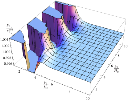
Figure 1: Power spectrum of the tensor mode $H_{\times}$ relative to the isotropic case. The high momentum mode corresponds to large $k_{1}/H_{0}$ and $k_{2}/H_{0}$. The planar mode corresponds to the case that $k_{1}/H_{0}$ becomes $O(1)$.

V.2 Mixed modes and power spectra

The evolution of $V$ and $H_{+}$ modes can be dealt with the parallel way. The evolution equations at the initial times are given in terms of the mixed form

$$\frac{d^{2}}{dt^{2}}\left(\begin{tabular}[]{c}$V$\\ $H_{+}$\\ \end{tabular}\right)+2^{4/3}\left[k_{1}^{2}{\bf 1}+\left(\begin{tabular}[]{cc}$\delta\omega_{11}^{2}$&$\delta\omega_{12}^{2}$\\ $\delta\omega_{12}^{2}$&$\delta\omega_{22}^{2}$\\ \end{tabular}\right)e^{6Ht}\right]\left(\begin{tabular}[]{c}$V$\\ $H_{+}$\\ \end{tabular}\right)=0,$$ (76)

where $\delta\omega^{2}$s are defined in Eq. (V). We may diagonalize the equation (76) by using the transformation

$$\left(\begin{tabular}[]{c}$V$\\ $H_{+}$\\ \end{tabular}\right)=O\left(\begin{tabular}[]{c}$v$\\ $h_{+}$\\ \end{tabular}\right)=\left(\begin{tabular}[]{cc}$\cos\psi$&$-\sin\psi$\\ $\sin\psi$&$\cos\psi$\\ \end{tabular}\right)\left(\begin{tabular}[]{c}$v$\\ $h_{+}$\\ \end{tabular}\right).$$

By choosing $\psi$ to be

$$\cos\psi = \Big{[}\frac{1}{2}\Big{(}1+\frac{1}{\sqrt{1+\chi_{0}^{2}}}\Big{)}\Big{]}^{\frac{1}{2}},\quad\sin\psi=\Big{[}\frac{1}{2}\Big{(}1-\frac{1}{\sqrt{1+\chi_{0}^{2}}}\Big{)}\Big{]}^{\frac{1}{2}},$$

$$\chi_{0} := \frac{2\delta\omega_{12}^{2}}{\delta\omega_{22}^{2}-\delta\omega_{11}^{2}}.$$ (77)

At the initial times, $\chi_{0}$ becomes

$$\chi_{0}=-\frac{2m/H_{0}}{\sqrt{3}(1-m^{2}/(6H_{0}^{2}))}+O(1/s^{2}).$$

Then the frequency term can be diagonalized

$$O^{-1}\left(\begin{tabular}[]{cc}$\delta\omega_{11}^{2}$&$\delta\omega_{12}^{2}$\\ $\delta\omega_{12}^{2}$&$\delta\omega_{22}^{2}$\\ \end{tabular}\right)O=\left(\begin{tabular}[]{cc}$\delta\tilde{\omega}{}_{11}^{2}$&$0$\\ $0$&$\delta\tilde{\omega}{}_{22}^{2}$\\ \end{tabular}\right),$$

where

$$\delta{\tilde{\omega}}_{11}^{2} = \frac{1}{2}\Big{(}\delta\omega_{11}^{2}+\delta\omega_{22}^{2}-\big{(}\delta\omega_{22}^{2}-\delta\omega_{11}^{2}\big{)}\sqrt{1+\frac{4(\delta\omega_{12}^{2})^{2}}{(\delta\omega_{11}^{2}-\delta\omega_{22}^{2})^{2}}}\Big{)},$$

$$\delta{\tilde{\omega}}_{22}^{2} = \frac{1}{2}\Big{(}\delta\omega_{11}^{2}+\delta\omega_{22}^{2}+\big{(}\delta\omega_{22}^{2}-\delta\omega_{11}^{2}\big{)}\sqrt{1+\frac{4(\delta\omega_{12}^{2})^{2}}{(\delta\omega_{11}^{2}-\delta\omega_{22}^{2})^{2}}}\Big{)}.$$ (78)

The original mixed equations are now diagonalized for the new variables

$${\cal M}=\left(\begin{tabular}[]{c}$v$\\ $h_{+}$\\ \end{tabular}\right)=\left(\begin{tabular}[]{c}$V\cos\psi+H_{+}\sin\psi$\\ $H_{+}\cos\psi-V\sin\psi$\\ \end{tabular}\right)\,.$$ (83)

The solutions are given by

$$v \approx \Big{(}1+\frac{m}{\sqrt{3}H_{0}}\Big{)}\sqrt{\frac{\pi}{6H_{0}\sinh(\pi q_{1})}}J_{-iq_{1}}\Big{(}q_{11}e^{3H_{0}t}\Big{)},$$

$$h_{+} \approx \Big{(}1-\frac{m}{\sqrt{3}H_{0}}\Big{)}\sqrt{\frac{\pi}{6H_{0}\sinh(\pi q_{1})}}J_{-iq_{1}}\Big{(}q_{22}e^{3H_{0}t}\Big{)},$$ (84)

where $q_{1}:=\frac{2^{\frac{2}{3}}|k_{1}|}{3H_{0}}$, $q_{11}:=\frac{2^{\frac{2}{3}}(\delta{\tilde{\omega}}_{11}^{2})^{\frac{1}{2}}}{3H_{0}}$, and $q_{22}:=\frac{2^{\frac{2}{3}}(\delta{\tilde{\omega}}_{22}^{2})^{\frac{1}{2}}}{3H_{0}}$, and similarly to the non-planar high momentum modes, factors of order $\frac{m}{H_{0}}$ represent corrections due to the initial mixing of modes and the early time limit of the above solutions correctly reproduces the normalized amplitude. Note that these solutions reproduce the correct normalizations in the limit $t\to-\infty$. By definition, $V$ and $H_{+}$ are now given by

$$V = \sqrt{\frac{\pi}{6H_{0}\sinh(\pi q_{1})}}\Big{[}\Big{(}1+\frac{m}{\sqrt{3}H_{0}}\Big{)}\cos\psi J_{-iq_{1}}\Big{(}q_{11}e^{3H_{0}t}\Big{)}$$

$$- \Big{(}1-\frac{m}{\sqrt{3}H_{0}}\Big{)}\sin\psi J_{-iq_{1}}\Big{(}q_{22}e^{3H_{0}t}\Big{)}\Big{]},$$

$$H_{+} = \sqrt{\frac{\pi}{6H_{0}\sinh(\pi q_{1})}}\Big{[}\Big{(}1+\frac{m}{\sqrt{3}H_{0}}\Big{)}\sin\psi J_{-iq_{1}}\Big{(}q_{11}e^{3H_{0}t}\Big{)}$$ (85)

$$+ \Big{(}1-\frac{m}{\sqrt{3}H_{0}}\Big{)}\cos\psi J_{-iq_{1}}\Big{(}q_{22}e^{3H_{0}t}\Big{)}\Big{]}.$$

When the WKB becomes valid, the coupling between $\tilde{V}$ and ${\tilde{H}}_{+}$ is negligible. At this time, we can match the solution Eq. (85) to WKB solutions. Then, when the universe enters into the de Sitter phase, we finally match the WKB solutions, to the de Sitter mode functions. The essential procedure is almost the same as the case of the $H_{\times}$ mode. The details are summarized in the Appendix B 2. In this subsection we only show the final results: The power spectrum of $\tilde{V}$ ($=V$) for the planar modes is given by

$$P_{V} \simeq P_{V}^{(0)}\Big{(}1+\frac{2m}{\sqrt{3}H_{0}}\Big{)}\Big{(}\coth(\pi q_{1})-\frac{\sin(2\Psi_{V,1})}{\sinh(\pi q_{1})}\Big{)},\quad$$ (86)

where

$$\Psi_{V,1}=\frac{\sqrt{\pi}\Gamma(\frac{1}{3})}{3\times 2^{\frac{1}{3}}\Gamma(\frac{5}{6})}\frac{k}{H_{0}}+O(\sqrt{\frac{k}{H_{0}}}).$$

Similarly, the power spectrum of ${\tilde{H}}_{+}$ ($=H_{+}$) for the planar modes is given by

$$P_{h_{+}} \simeq P_{h_{+}}^{(0)}\Big{(}1-\frac{2m}{\sqrt{3}H_{0}}\Big{)}\Big{(}\coth(\pi q_{1})-\frac{\sin(2\Psi_{+,2})}{\sinh(\pi q_{1})}\Big{)},$$

$$\Psi_{+,2} := \frac{\sqrt{\pi}\Gamma(\frac{1}{3})}{3\times 2^{\frac{1}{3}}\Gamma(\frac{5}{6})}\frac{k}{H_{0}}+O(\sqrt{\frac{k}{H_{0}}}).$$ (87)

Note that the forms of the power spectra for the $H_{+}$ and $V$ modes are almost the same as that of the $H_{\times}$ mode except for the global scaling due to the initial mode mixing.

VI Conclusion

In this paper, we have analytically investigated the corrections to the power spectra of the cosmological perturbations due to the preinflationary anisotropy of the universe, for the high momentum modes in the context of WKB approximations. The first motivation to consider the anisotropic universe is that even if the present universe is almost isotropic, it does not mean that it is also isotropic from the beginning. It would be more generic that the initial universe is highly anisotropic. The second motivation comes from observations. In recent years, several groups have reported the so-called low-$\ell$ anomalies in large angular power of CMB fluctuations. They may be produced by the breaking of the rotational symmetry in the early universe.

We considered the Einstein gravity coupled to a light scalar field. We assumed that this scalar field initially stays at a very large (super-Planck) field value, and then starts to roll down slowly. If the mass of the scalar field is small enough, the kinetic energy of the scalar field does not affect the spacetime dynamics significantly. Imposing the regularity of the spacetime at the initial time, one of two planar branches of the Kasner-de Sitter solution, whose initial geometry becomes a (Milne) patch of the Minkowski spacetime, is a good approximation for describing the cosmic isotropization. The cosmic isotropization takes place within a few Hubble times. During the subsequent inflationary stage, the scalar field rolls down toward the true minimum and plays the role of the inflaton.

Then, we investigated the analytic expressions for the spectra of the cosmological perturbations produced in the above anisotropic background for the high momentum modes. In the anisotropic background, there are 2 scalar and 1 vector modes in terms of the two-dimensional flat space. In the isotropic limit, this vector mode in the anisotropic universe reduces to one of tensor polarizations in the flat 3-dimensional space, while two scalar modes reduce to one scalar and the other tensor polarization there. During the anisotropic phase, two scalar modes are coupled, resulting in the asymmetry between the spectra of two tensor polarizations obtained in the isotropic limit. Since at the initial times, the coupling is absent, we could define the adiabatic vacuum, which we call the anisotropic vacuum, and canonically quantize the perturbations. Our anisotropic vacuum is definitely different from the standard Bunch-Davis vacuum. In addition, the presence of the anisotropic vacuum is specific to our particular choice of the Kasner parameter.

For the non-planar modes $k,k_{1}\gg H_{0}$, for the sufficiently high momentum the WKB approximation is valid but the mixing angle does not vanish at the early time. At the leading order, the power spectra of all the perturbation modes contain the corrections due to the nonstandard propagation in the anisotropic background, and the effects of the initial mixing of modes. The former has the universal form, while the latter induces an asymmetry of two gravitational wave polarizations in the isotropic limit. The modifications of spectra appear in the oscillatory behaviors of the primordial spectrum. On the other hand, for the planar mode, i.e., $k\gg k_{1}\sim H_{0}$, although the WKB approximation is broken at the very early times, the mode mixing does not take place significantly. For the modes of $k_{1}=0$, the adiabaticity parameter initially diverges and hence the anisotropic vacuum is not well defined. However, such modes are not relevant for the observations.

One of the main results which we have obtained is that, irrespective of the non-planar or planar modes, for the high momentum modes the ratio of the power spectra between two tensor polarizations is given by

$$\frac{P_{h_{+}}}{P_{h_{\times}}}\approx 1-\frac{2m}{\sqrt{3}H_{0}}.$$ (88)

In the chaotic inflation typically $\frac{m}{H_{0}}=O(0.1)$, and hence there is a difference of the spectra of two gravitational wave polarizations, which is of roughly ten percent.

Before closing this article, it may be important to mention the effects of the primordial anisotropy on the higher order spectra, in particular on the bispectrum, and the primordial non-Gaussianities. In the model discussed in this paper the initial vacuum is not the standard Bunch-Davis vacuum, and the subsequent evolution is almost the same as that in the single field, slow-roll inflation. Thus, we expect that the folded shape bispectrum where three momenta satisfy $k_{1}+k_{2}\sim k_{3}$ would become dominant chen ; chks (see also isca ), while the local shape bispectrum of $k_{2}\sim k_{3}\gg k_{1}$ would be negligible jm . However, the particular local type bispectrum where $k_{2}$ and $k_{3}$ almost lie in the plane of the $y$ and $z$ directions of Eq. (2) while $k_{1}$ is nearly orthogonal to this plane ($k_{2}\sim k_{3}\gg k_{1}$), could be much different from the case of the isotropic universe, since as in the case of the spectra for the planar modes it could be sensitive to the anisotropy. For the non-planar case of $k_{1}+k_{2}\sim k_{3}$, the amount of the non-Gaussianities would be determined by the coefficient $B_{\tilde{V}}$ in Eq. (61) which represents the amplitude of the negative frequency mode;

$${\rm Re}(B_{\tilde{V}})\sim Q(r_{2})\Big{(}\frac{H_{0}}{k}\Big{)}^{\frac{3}{2}}\sin\big{(}\sqrt{\frac{k}{H_{0}}}+\phi_{0}\big{)},$$ (89)

where $\phi_{0}$ denotes some constant phase. Note that due to the effect of the initial mode mixing ${\rm Re}(B_{\tilde{V}})$ may be amplified by some factor of order $\frac{m}{H_{0}}\sim 0.1$. Therefore, the bispectrum could exhibit an oscillatory behavior, and contain the information on the primordial anisotropy through the factor $Q(r_{2})$, which may be distinguishable if detected. The concrete evaluation of the bispectrum in the anisotropic universe and the detectability of the non-Gaussianities will be interesting issues and should be investigated in the future studies.

Appendix A On the power spectra for the non-planar, high-momentum modes

We will summarize the matching of the WKB and de Sitter mode functions for the non-planar high momentum modes, given by Eqs. (58) and (61), respectively.

Keeping the accuracy to the second order in adiabatic approximation, the solution to Eq. (59) is given by

$$\Omega=\omega(1+\delta),$$ (90)

where

$$\delta:=-\frac{1}{4\omega^{2}}\Big{(}\frac{\omega_{,tt}}{\omega}-\frac{3\omega_{,t}^{2}}{2\omega^{2}}\Big{)}.$$

Defining

$$a:=1-\frac{\delta}{2},\quad b:=1+\frac{\delta}{2},\quad c:=-\frac{\omega_{,t}}{2\omega^{2}}\Big{(}1-\frac{\delta}{2}+\frac{\omega\delta_{,t}}{\omega_{,t}}\Big{)},$$ (91)

and using the results of matching at some appropriate time $t=t_{\ast}$, the final power spectrum is given by

$$P_{\tilde{Y}} = P_{\tilde{Y}}^{(0)}\frac{K_{Y}}{\nu_{\ast}}\Big{\{}b^{2}\nu_{\ast}^{2}\Big{(}\cos\big{[}\frac{k}{H_{0}}(-3H_{0}t_{\ast})^{\frac{1}{3}}\big{]}-\frac{H_{0}}{k}\frac{1}{(-3H_{0}t)^{\frac{1}{3}}}\sin\big{[}\frac{k}{H_{0}}(-3H_{0}t_{\ast})^{\frac{1}{3}}\big{]}\Big{)}^{2}$$ (92)

$$+ \Big{(}-\big{(}a+c\frac{H}{k}\frac{\nu_{\ast}}{(-3H_{0}t_{\ast})^{\frac{1}{3}}}\big{)}\sin\big{[}\frac{k}{H_{0}}(-3H_{0}t_{\ast})^{\frac{1}{3}}\big{]}+c\nu_{\ast}\cos\big{[}\frac{k}{H_{0}}(-3H_{0}t_{\ast})^{\frac{1}{3}}\big{]}\Big{)}^{2}\Big{\}},$$

where $\nu_{\ast}:=\frac{\omega_{\ast}}{k}(-3H_{0}t_{\ast})^{\frac{2}{3}}$ and $\Phi=\int^{t_{\ast}}dt^{\prime}\omega(t^{\prime})$, and $P_{Y}^{(0)}$ is given by (36). $K_{\tilde{Y}}$ represents the contribution of the initial mixing of modes, which are given by $K_{\times}=1$, $K_{V}=1+\frac{2m}{\sqrt{3}H_{0}}$ and $K_{+}=1-\frac{2m}{\sqrt{3}H_{0}}$.

For all ${\tilde{H}}_{+}$, ${\tilde{V}}$ and $H_{\times}$ modes, we obtain in the high momentum limit,

$$\omega_{\ast}^{2}=k^{2}e^{4\alpha}\Big{(}1+2e^{-3\alpha}Q(r_{2})\Big{)}+O(m^{2}),$$ (93)

where $Q(r_{2}):=\frac{2}{3}-r_{2}^{2}$ ($r_{2}:=\frac{k_{2}}{k}$) denotes the leading order corrections due to the anisotropy. Note that $-\frac{1}{3}\leq Q(r_{2})\leq\frac{2}{3}$ and $O(m^{2})$ terms contain the slow-roll corrections. Thus, as long as our concerns are in the high momentum modes, $O(m^{2})$ terms are not important. The WKB approximations are valid as long as the adiabaticity parameter Eq (55) is smaller than unity, namely $-H_{0}t\gg\Big{(}\frac{H_{0}}{k}\Big{)}^{3}$. On the other hand, the late time approximation is valid if $e^{\alpha}\gg 1$. The matching time $t=t_{\ast}$ should be chosen so that the error is minimized and is given in terms of their geometric mean km :

$$e^{\alpha}\Big{|}_{t=t_{\ast}}:=\Big{(}\frac{k}{H_{0}}\Big{)}^{\frac{1}{2}}.$$ (94)

At $t=t_{*}$, $\epsilon_{{\tilde{Y}},\ast}\simeq\frac{H_{0}^{\frac{1}{2}}}{k^{\frac{1}{2}}}$. Making use of $(-3H_{0}t_{\ast})^{\frac{1}{3}}=\Big{(}\frac{H_{0}}{k}\Big{)}^{\frac{1}{2}}\Big{[}1+O(\frac{k^{3}}{H_{0}^{3}})\Big{]}.$ the power spectrum is given by

$$P_{\tilde{Y}} = P_{\tilde{Y}}^{(0)}\frac{K_{Y}}{\nu_{\ast}}\Big{\{}b^{2}\nu_{\ast}^{2}\Big{(}\cos\sqrt{\frac{k}{H_{0}}}-\sqrt{\frac{H_{0}}{k}}\sin\sqrt{\frac{k}{H_{0}}}\Big{)}^{2}$$ (95)

$$+ \Big{(}-\big{(}a+c\nu_{\ast}\sqrt{\frac{H_{0}}{k}}\big{)}\sin\sqrt{\frac{k}{H_{0}}}+c\nu_{\ast}\cos\sqrt{\frac{k}{H_{0}}}\Big{)}^{2}\Big{\}}.$$

As shown in the previous section, $\sin\theta$ is $O(m/H_{0})$ at early times and vanishes at late times, and thus the initial condition for $V$ and $H_{+}$ modes will be specified by using the WKB approximation for $\tilde{V}$ and $\tilde{H}_{+}$. Since $\tilde{V}=V$ and $\tilde{H}_{+}=H_{+}$ at $t\to 0-$, the power spectra for $\tilde{Y}$ reproduce those of $Y$. Therefore, $P_{Y}=P_{\tilde{Y}}$.

Then, evaluating at $t=t_{1}$ up to $O\Big{(}\big{(}\frac{H_{0}}{k}\big{)}^{2}\Big{)}$,

$$\nu_{\ast}=1+Q(r_{2})\Big{(}\frac{H_{0}}{k}\Big{)}^{\frac{3}{2}}+O\Big{(}\Big{(}\frac{H_{0}}{k}\Big{)}^{2}\Big{)},\quad a=1+\frac{H_{0}}{2k}+O\Big{(}\Big{(}\frac{H_{0}}{k}\Big{)}^{2}\Big{)},$$

$$b=1-\frac{H_{0}}{2k}+O\Big{(}\Big{(}\frac{H_{0}}{k}\Big{)}^{2}\Big{)},\quad c=-\sqrt{\frac{H_{0}}{k}}\Big{(}1-\frac{H_{0}}{2k}\Big{)}+O\Big{(}\Big{(}\frac{H_{0}}{k}\Big{)}^{2}\Big{)}.$$ (96)

Therefore, we obtain the power spectrum including the leading order corrections from the direction dependent part

$$P_{\times} = P_{\times}^{(0)}\Big{[}1+Q(r_{2})\Big{(}\frac{H_{0}}{k}\Big{)}^{\frac{3}{2}}\cos\Big{(}2\sqrt{\frac{k}{H_{0}}}\Big{)}+O\Big{(}\Big{(}\frac{H_{0}}{k}\Big{)}^{2}\Big{)}\Big{]},$$

$$P_{V} = P_{V}^{(0)}\Big{[}1+\frac{2m}{\sqrt{3}H_{0}}+Q(r_{2})\Big{(}\frac{H_{0}}{k}\Big{)}^{\frac{3}{2}}\cos\Big{(}2\sqrt{\frac{k}{H_{0}}}\Big{)}+O\Big{(}\Big{(}\frac{H_{0}}{k}\Big{)}^{2}\Big{)}\Big{]},$$

$$P_{+} = P_{+}^{(0)}\Big{[}1-\frac{2m}{\sqrt{3}H_{0}}+Q(r_{2})\Big{(}\frac{H_{0}}{k}\Big{)}^{\frac{3}{2}}\cos\Big{(}2\sqrt{\frac{k}{H_{0}}}\Big{)}+O\Big{(}\Big{(}\frac{H_{0}}{k}\Big{)}^{2}\Big{)}\Big{]}.$$ (97)

Appendix B On the power spectra of the planar modes

B.1 On $H_{\times}$

Here, we explain the derivation of the power spectrum of $H_{\times}$ for the planar modes.

For $H_{0}t\ll-1$, the solutions for $H_{\times}$ are given by

$$H^{(1)}_{\times}=\sqrt{\frac{\pi}{6H_{0}\sinh(\pi q_{1})}}J_{-iq_{1}}\Big{(}q_{\times}e^{3H_{0}t}\Big{)},$$ (98)

where $q_{1}:=\frac{2^{\frac{2}{3}}k_{1}}{3H_{0}}$ and $q_{\times}:=\frac{2^{\frac{2}{3}}(\delta\omega_{\times}^{2})^{\frac{1}{2}}}{3H_{0}}$. Note that this solution reproduces the correct normalization in the limit $t\to-\infty$. During the period of time $2t_{1,\times}<t\ll-\frac{H_{0}^{2}}{k^{3}}$, where $t_{1}$ is the matching time given below, the WKB approximation

$$H^{(2)}_{\times}=\frac{B_{\times,+}}{\sqrt{2\omega_{\times}}}{\rm exp}\Big{[}-i\int_{t_{1,\times}}^{t}dt^{\prime}\omega_{\times}(t^{\prime})\Big{]}+\frac{B_{\times,-}}{\sqrt{2\omega_{\times}}}{\rm exp}\Big{[}i\int_{t_{1,\times}}^{t}dt^{\prime}\omega_{\times}(t^{\prime})\Big{]},$$ (99)

holds well. In order for the error to be minimized, we need to choose the matching time of the two solutions (98) and (99), $t=t_{1,\times}$ to be

$$e^{3H_{0}t_{1,\times}}\simeq\frac{3}{2^{\frac{2}{3}}}\sqrt{\frac{H_{0}}{(\delta\omega_{\times}^{2})^{\frac{1}{2}}}},$$ (100)

since the adiabaticity parameter behaves as $\epsilon_{\times}\simeq\frac{3\times 2^{\frac{1}{3}}H_{0}}{(\delta\omega_{\times}^{2})^{\frac{1}{2}}}e^{-3H_{0}t}$. Since $q_{\times}e^{3H_{0}t_{1,\times}}\gg 1$ at $t=t_{1}$,

$$H^{(1)}_{\times}\simeq\sqrt{\frac{1}{3H_{0}q_{\times}e^{3H_{0}t}\sinh(\pi q_{1})}}\sin\Upsilon_{\times},$$ (101)

where $\Upsilon_{\times}=q_{\times}e^{3H_{0}t}+\frac{\pi}{4}+\frac{iq_{1}\pi}{2}$. Noting

$$\frac{3H_{0}q_{\times}e^{3Ht_{1,\times}}}{\omega_{\times}|_{t=t_{1,\times}}}=\Big{(}1+\frac{H_{0}q_{1}^{2}}{\big{(}\delta\omega_{\times}^{2}\big{)}^{\frac{1}{2}}}\Big{)}^{-\frac{1}{2}},$$ (102)

we obtain

$$B_{\times,+} = \sqrt{\frac{\omega_{\times}|_{t=t_{1,\times}}}{2}}\Big{(}H_{\times}^{(1)}+i\frac{H^{(1)}_{\times,t}}{\omega_{\times}}\Big{)}_{t=t_{1,\times}}$$

$$\simeq \frac{i}{\sqrt{2\sinh(\pi q_{1})}}\Big{[}\Big{(}1+\frac{H_{0}q_{1}^{2}}{\big{(}\delta\omega_{\times}^{2}\big{)}^{\frac{1}{2}}}\Big{)}^{-\frac{1}{4}}\cos\Upsilon_{\times}|_{t=t_{1,\times}}-i\Big{(}1+\frac{H_{0}q_{1}^{2}}{\big{(}\delta\omega_{\times}^{2}\big{)}^{\frac{1}{2}}}\Big{)}^{\frac{1}{4}}\sin\Upsilon_{\times}\big{|}_{t=t_{1,\times}}\Big{]},$$

$$B_{\times,-} = \sqrt{\frac{\omega_{\times}|_{t=t_{1,\times}}}{2}}\Big{(}H_{\times}^{(1)}-i\frac{H^{(1)}_{\times,t}}{\omega_{\times}}\Big{)}_{t=t_{1,\times}}$$ (103)

$$\simeq \frac{(-i)}{\sqrt{2\sinh(\pi q_{1})}}\Big{[}\Big{(}1+\frac{H_{0}q_{1}^{2}}{\big{(}\delta\omega_{\times}^{2}\big{)}^{\frac{1}{2}}}\Big{)}^{-\frac{1}{4}}\cos\Upsilon_{\times}|_{t=t_{1,\times}}+i\Big{(}1+\frac{H_{0}q_{1}^{2}}{\big{(}\delta\omega_{\times}^{2}\big{)}^{\frac{1}{2}}}\Big{)}^{\frac{1}{4}}\sin\Upsilon_{\times}\big{|}_{t=t_{1,\times}}\Big{]}.$$

Since $q_{1}^{2}\ll\frac{H_{0}}{(\delta\omega_{\times}^{2})^{\frac{1}{2}}}$, at the leading order they reduce to

$$B_{\times,+}\simeq\frac{1}{(1-e^{-2\pi q_{1}})^{\frac{1}{2}}}e^{i\big{(}\frac{\pi}{4}-\sqrt{\frac{(\delta\omega_{\times}^{2})^{\frac{1}{2}}}{H_{0}}}\big{)}},\quad B_{\times,-}\simeq\frac{e^{-\pi q_{1}}}{(1-e^{-2\pi q_{1}})^{\frac{1}{2}}}e^{-i\big{(}\frac{\pi}{4}-\sqrt{\frac{(\delta\omega_{\times}^{2})^{\frac{1}{2}}}{H_{0}}}\big{)}}.$$ (104)

Then, at $t=t_{\ast}$ ($|t_{\ast}|\ll|t_{1,\times}|$), where $t_{\ast}$ is chosen to be Eq. (94) as for the non-planar modes, the WKB solution are matched to the de Sitter mode function

$$H^{(3)}_{\times} = \frac{C_{\times,+}}{\sqrt{2k}}e^{i\frac{k}{H_{0}}(-3H_{0}t)^{\frac{1}{3}}}\Big{[}\big{(}-3H_{0}t\big{)}^{\frac{1}{3}}+\frac{iH_{0}}{k}\Big{]}+\frac{C_{\times,-}}{\sqrt{2k}}e^{-i\frac{k}{H_{0}}(-3H_{0}t)^{\frac{1}{3}}}\Big{[}\big{(}-3H_{0}t\big{)}^{\frac{1}{3}}-\frac{iH_{0}}{k}\Big{]}.$$ (105)

$$\xrightarrow[t\to 0-]{} \frac{iH_{0}}{\sqrt{2k^{3}}}\Big{(}C_{\times,+}-C_{\times,-}\Big{)}.$$

For the high momentum modes,

$$C_{\times,+}\simeq e^{-i\sqrt{\frac{k}{H_{0}}}}e^{-i\Phi}B_{\times,+},\quad C_{\times,-}\simeq e^{i\sqrt{\frac{k}{H_{0}}}}e^{i\Phi}B_{\times,-},$$ (106)

where $\Phi=\int_{t_{1,\times}}^{t_{\ast}}dt^{\prime}\omega_{\times}(t^{\prime})$. Thus,

$$C_{\times,+}-C_{\times,-}=\frac{1}{(1-e^{-2\pi q_{1}})^{\frac{1}{2}}}\Big{\{}\big{(}1-e^{-\pi q_{1}}\big{)}\cos\big{(}\frac{\pi}{4}-\Psi_{\times}\big{)}+i\big{(}1+e^{-\pi q_{1}}\big{)}\sin\big{(}\frac{\pi}{4}-\Psi_{\times}\big{)}\Big{\}},$$ (107)

where $\Psi_{\times}:=\sqrt{\frac{(\delta\omega^{2}_{\times})^{\frac{1}{2}}}{H_{0}}}+\Phi+\sqrt{\frac{k}{H_{0}}}$. Therefore, the power spectrum for the $H_{\times}$ mode is given by

$$P_{h_{\times}} \simeq P_{h_{\times}}^{(0)}\Big{(}\coth\big{(}\pi q_{1}\big{)}-\frac{\sin(2\Psi_{\times})}{\sinh(\pi q_{1})}\Big{)}.$$ (108)

Finally, we estimate $\Psi_{\times}$. From Eq. (67),

$$\Phi=\int_{t_{1,\times}}^{t_{\ast}}dt\frac{2^{\frac{2}{3}}k_{2}e^{3H_{0}t}}{(1-e^{6H_{0}t})^{\frac{2}{3}}}=\frac{2^{\frac{2}{3}}k_{2}}{3H_{0}}e^{3H_{0}t}{}_{2}F_{1}\Big{[}\frac{1}{2},\frac{2}{3},\frac{3}{2},e^{6H_{0}t}\Big{]}\Big{|}_{t_{1,\times}}^{t_{\ast}}\simeq\frac{\sqrt{\pi}\Gamma(\frac{1}{3})}{3\times 2^{\frac{1}{3}}\Gamma(\frac{5}{6})}\frac{k_{2}}{H_{0}},$$ (109)

and the $\Phi$ term dominates $\Psi_{\times}$:

$$\Psi_{\times}=\frac{\sqrt{\pi}\Gamma(\frac{1}{3})}{3\times 2^{\frac{1}{3}}\Gamma(\frac{5}{6})}\frac{k}{H_{0}}+O(\sqrt{\frac{k}{H_{0}}}).$$

Here we use the fact that $k_{2}\simeq k$ in the case of planar modes.

B.2 On $V$ and $H_{+}$

Similarly, we explain the derivation of the power spectra of $V$ and $H_{+}$ for the planar modes. Firstly, we match the solutions Eq. (85) to the WKB solutions, and then match them to the mode functions in the de Sitter inflation. Most computations are the same as in the case of $H_{\times}$.

B.2.1 $\tilde{V}$ mode

At the time when the WKB becomes valid, the coupling between $\tilde{V}$ and ${\tilde{H}}_{+}$ is negligible. At $t=t_{1,V}$ given by

$$e^{3H_{0}t_{1,V}}\simeq\frac{3}{2^{\frac{2}{3}}}\sqrt{\frac{H_{0}}{(\delta{\tilde{\omega}}_{11}^{2})^{\frac{1}{2}}}},$$ (110)

the asymptotic form of the first solution

$${\tilde{V}} \simeq \sqrt{\frac{1}{e^{3H_{0}t}\sinh(\pi q_{1})}}\Big{[}\Big{(}1+\frac{m}{\sqrt{3}H_{0}}\Big{)}\frac{\cos\big{(}\psi-\theta\big{)}}{2^{\frac{1}{3}}(\delta{\tilde{\omega}}_{11}^{2})^{\frac{1}{4}}}\sin\Upsilon_{11}$$ (111)

$$- \Big{(}1-\frac{m}{\sqrt{3}H_{0}}\Big{)}\frac{\sin\big{(}\psi-\theta\big{)}}{2^{\frac{1}{3}}(\delta{\tilde{\omega}}_{22}^{2})^{\frac{1}{4}}}\cos\Upsilon_{22}\Big{]},$$

where $\Upsilon_{11}=q_{11}e^{3H_{0}t}+\frac{\pi}{4}+\frac{iq_{1}\pi}{2}$ and $\Upsilon_{22}=q_{22}e^{3H_{0}t}+\frac{\pi}{4}+\frac{iq_{1}\pi}{2}$, is matched to the WKB solution given by

$${\tilde{V}}^{(2)}=\frac{B_{V,+}}{\sqrt{2{\tilde{\omega}}_{11}}}{\rm exp}\Big{[}-i\int_{t_{1,V}}^{t}dt^{\prime}{\tilde{\omega}}_{11}(t^{\prime})\Big{]}+\frac{B_{V,-}}{\sqrt{2{\tilde{\omega}}_{11}}}{\rm exp}\Big{[}i\int_{t_{1,V}}^{t}dt^{\prime}{\tilde{\omega}}_{11}(t^{\prime})\Big{]}.$$ (112)

Since from Eqs. (45) and (77), at $t=t_{1,V}$

$$\chi\Big{|}_{t=t_{1,V}}=\frac{2\omega_{12}^{2}}{\omega_{22}^{2}-\omega_{11}^{2}}\Big{|}_{t=t_{1,V}}\simeq\frac{2\delta\omega_{12}^{2}}{\delta\omega_{22}^{2}-\delta\omega_{11}^{2}}=\chi_{0},$$ (113)

at the leading order, we obtain $\psi\approx\theta_{1,V}$. The first solution then reduces to

$${\tilde{V}} \simeq \sqrt{\frac{1}{e^{3H_{0}t}\sinh(\pi q_{1})}}\Big{(}1+\frac{m}{\sqrt{3}H_{0}}\Big{)}\frac{1}{2^{\frac{1}{3}}(\delta{\tilde{\omega}}_{11}^{2})^{\frac{1}{4}}}\sin\Upsilon_{11}.$$ (114)

Noting that $q_{11}^{2}\ll\frac{(\delta{\tilde{\omega}}_{11}^{2})^{\frac{1}{2}}}{H_{0}}$, after matching these solutions, we obtain

$$B_{V,+} \simeq \frac{1}{(1-e^{-2\pi q_{1}})^{\frac{1}{2}}}\Big{(}1+\frac{m}{\sqrt{3}H_{0}}\Big{)}e^{i\big{(}\frac{\pi}{4}-\sqrt{\frac{(\delta{\tilde{\omega}}_{11}^{2})^{\frac{1}{2}}}{H_{0}}}\big{)}},$$

$$B_{V,-} \simeq \frac{e^{-\pi q_{1}}}{(1-e^{-2\pi q_{1}})^{\frac{1}{2}}}\Big{(}1+\frac{m}{\sqrt{3}H_{0}}\Big{)}e^{-i\big{(}\frac{\pi}{4}-\sqrt{\frac{(\delta{\tilde{\omega}}_{11}^{2})^{\frac{1}{2}}}{H_{0}}}\big{)}}.$$ (115)

Then, at $t=t_{\ast}$ ($|t_{\ast}|\ll|t_{1,V}|$), where $t_{\ast}$ is chosen to be Eq. (94) as for the non-planar high momentum modes, the WKB solution are matched to the de Sitter mode function

$${\tilde{V}}^{(3)} = \frac{C_{V,+}}{\sqrt{2k}}e^{i\frac{k}{H_{0}}(-3H_{0}t)^{\frac{1}{3}}}\Big{[}\big{(}-3H_{0}t\big{)}^{\frac{1}{3}}+\frac{iH_{0}}{k}\Big{]}+\frac{C_{V,-}}{\sqrt{2k}}e^{-i\frac{k}{H_{0}}(-3H_{0}t)^{\frac{1}{3}}}\Big{[}\big{(}-3H_{0}t\big{)}^{\frac{1}{3}}-\frac{iH_{0}}{k}\Big{]}$$ (116)

$$\xrightarrow[t\to 0-]{} \frac{iH_{0}}{\sqrt{2k^{3}}}\Big{(}C_{V,+}-C_{V,-}\Big{)}.$$

For the high momentum modes,

$$C_{V,+}-C_{V,-}\simeq\frac{1+\frac{m}{\sqrt{3}H_{0}}}{(1-e^{-2\pi q_{1}})^{\frac{1}{2}}}\Big{\{}\big{(}1-e^{-\pi q_{1}}\big{)}\cos\big{(}\frac{\pi}{4}-\Psi_{V,1}\big{)}+i\big{(}1+e^{-\pi q_{1}}\big{)}\sin\big{(}\frac{\pi}{4}-\Psi_{V,1}\big{)}\Big{\}},$$ (117)

where $\Psi_{V,1}:=\sqrt{\frac{(\delta{\tilde{\omega}}^{2}_{11})^{\frac{1}{2}}}{H_{0}}}+\Phi+\sqrt{\frac{k}{H_{0}}}$ and $\Psi_{V,2}:=\sqrt{\frac{(\delta{\tilde{\omega}}^{2}_{22})}{H_{0}(\delta{\tilde{\omega}}^{2}_{11})^{\frac{1}{2}}}}+\Phi+\sqrt{\frac{k}{H_{0}}}$. Thus, the power spectrum for the $\tilde{V}$ ($=V$) mode is given by

$$P_{V} \simeq P_{V}^{(0)}\Big{(}1+\frac{2m}{\sqrt{3}H_{0}}\Big{)}\Big{(}\coth(\pi q_{1})-\frac{\sin(2\Psi_{V,1})}{\sinh(\pi q_{1})}\Big{)},\quad$$ (118)

where the $\Phi$ term dominates $\Psi_{V,1}$ and

$$\Psi_{V,1}=\frac{\sqrt{\pi}\Gamma(\frac{1}{3})}{3\times 2^{\frac{1}{3}}\Gamma(\frac{5}{6})}\frac{k}{H_{0}}+O(\sqrt{\frac{k}{H_{0}}}).$$

Here we use the fact that $k_{2}\simeq k$ in the case of planar modes.

B.2.2 ${\tilde{H}}_{+}$ mode

Similarly for the ${\tilde{H}}_{+}$ mode, at $t=t_{1,+}$

$$e^{3H_{0}t_{1,+}}\simeq\frac{3}{2^{\frac{2}{3}}}\sqrt{\frac{H_{0}}{(\delta{\tilde{\omega}}_{22}^{2})^{\frac{1}{2}}}},$$ (119)

the asymptotic form of the first solution

$${\tilde{H}}_{+} \simeq \sqrt{\frac{1}{e^{3H_{0}t}\sinh(\pi q_{1})}}\Big{[}\Big{(}1+\frac{m}{\sqrt{3}H_{0}}\Big{)}\frac{\sin\big{(}\psi-\theta\big{)}}{2^{\frac{1}{3}}(\delta{\tilde{\omega}}_{11}^{2})^{\frac{1}{4}}}\sin\Upsilon_{11}$$ (120)

$$+ \Big{(}1-\frac{m}{\sqrt{3}H_{0}}\Big{)}\frac{\cos\big{(}\psi-\theta\big{)}}{2^{\frac{1}{3}}(\delta{\tilde{\omega}}_{22}^{2})^{\frac{1}{4}}}\cos\Upsilon_{22}\Big{]},$$

is matched to the WKB solution is given by

$${\tilde{H}}_{+}^{(2)}=\frac{B_{+,+}}{\sqrt{2{\tilde{\omega}}_{22}}}{\rm exp}\Big{[}-i\int_{t_{1,+}}^{t}dt^{\prime}{\tilde{\omega}}_{22}(t^{\prime})\Big{]}+\frac{B_{+,-}}{\sqrt{2{\tilde{\omega}}_{22}}}{\rm exp}\Big{[}i\int_{t_{1,+}}^{t}dt^{\prime}{\tilde{\omega}}_{22}(t^{\prime})\Big{]}.$$ (121)

From Eqs. (45) and (77), at $t=t_{{1,+}}$ the similar relation to Eq. (113) is obtained, which leads to $\psi\approx\theta_{1,+}$. Thus, the first solution reduces to

$${\tilde{H}}_{+} \simeq \sqrt{\frac{1}{e^{3H_{0}t}\sinh(\pi q_{1})}}\Big{(}1-\frac{m}{\sqrt{3}H_{0}}\Big{)}\frac{1}{2^{\frac{1}{3}}(\delta{\tilde{\omega}}_{22}^{2})^{\frac{1}{4}}}\cos\Upsilon_{22}.$$ (122)

Noting $q_{22}^{2}\ll\frac{(\delta{\tilde{\omega}}_{22}^{2})^{\frac{1}{2}}}{H_{0}}$, after matching these solutions, at the leading order we obtain the coefficients

$$B_{+,+} \simeq \frac{1}{(1-e^{-2\pi q_{1}})^{\frac{1}{2}}}\Big{(}1-\frac{m}{\sqrt{3}H_{0}}\Big{)}e^{i\big{(}\frac{\pi}{4}-\sqrt{\frac{(\delta{\tilde{\omega}}_{22}^{2})^{\frac{1}{2}}}{H_{0}}}\big{)}},$$

$$B_{+,-} \simeq \frac{e^{-\pi q_{1}}}{(1-e^{-2\pi q_{1}})^{\frac{1}{2}}}\Big{(}1-\frac{m}{\sqrt{3}H_{0}}\Big{)}e^{-i\big{(}\frac{\pi}{4}-\sqrt{\frac{(\delta{\tilde{\omega}}_{22}^{2})^{\frac{1}{2}}}{H_{0}}}\big{)}}.$$ (123)

Then, at $t=t_{\ast}$ with ($|t_{\ast}|\ll|t_{1,+}|$), where $t_{\ast}$ is chosen to be Eq. (94) as for the non-planar high momentum modes, the WKB solution are matched to the de Sitter mode function

$${\tilde{H}}_{+}^{(3)} = \frac{C_{+,+}}{\sqrt{2k}}e^{i\frac{k}{H_{0}}(-3H_{0}t)^{\frac{1}{3}}}\Big{[}\big{(}-3H_{0}t\big{)}^{\frac{1}{3}}+\frac{iH_{0}}{k}\Big{]}+\frac{C_{+,-}}{\sqrt{2k}}e^{-i\frac{k}{H_{0}}(-3H_{0}t)^{\frac{1}{3}}}\Big{[}\big{(}-3H_{0}t\big{)}^{\frac{1}{3}}-\frac{iH_{0}}{k}\Big{]}$$ (124)

$$\xrightarrow[t\to 0-]{} \frac{iH_{0}}{\sqrt{2k^{3}}}\Big{(}C_{+,+}-C_{+,-}\Big{)}.$$

For the high momentum modes,

$$C_{+,+}-C_{+,-}\simeq\frac{1-\frac{m}{\sqrt{3}H_{0}}}{(1-e^{-2\pi q_{1}})^{\frac{1}{2}}}\Big{\{}\big{(}1-e^{-\pi q_{1}}\big{)}\cos\big{(}\frac{\pi}{4}-\Psi_{+,2}\big{)}+i\big{(}1+e^{-\pi q_{1}}\big{)}\sin\big{(}\frac{\pi}{4}-\Psi_{+,2}\big{)}\Big{\}},$$ (125)

where $\Psi_{+,1}:=\sqrt{\frac{(\delta{\tilde{\omega}}^{2}_{11})}{H_{0}(\delta{\tilde{\omega}}^{2}_{22})^{\frac{1}{2}}}}+\Phi+\sqrt{\frac{k}{H_{0}}}$ and $\Psi_{+,2}:=\sqrt{\frac{(\delta{\tilde{\omega}}^{2}_{22})^{\frac{1}{2}}}{H_{0}}}+\Phi+\sqrt{\frac{k}{H_{0}}}$. Thus, the power spectrum for the ${\tilde{H}}_{+}$ ($=H_{+}$) mode is given by

$$P_{h_{+}} \simeq P_{h_{+}}^{(0)}\Big{(}1-\frac{2m}{\sqrt{3}H_{0}}\Big{)}\Big{(}\coth(\pi q_{1})-\frac{\sin(2\Psi_{+,2})}{\sinh(\pi q_{1})}\Big{)},$$

$$\Psi_{+,2} = \frac{\sqrt{\pi}\Gamma(\frac{1}{3})}{3\times 2^{\frac{1}{3}}\Gamma(\frac{5}{6})}\frac{k}{H_{0}}+O(\sqrt{\frac{k}{H_{0}}}).$$ (126)

Here we use the fact that $k_{2}\simeq k$ in the case of planar modes.

References

- (1) E. Komatsu et al. [WMAP Collaboration], Astrophys. J. Suppl. 180, 330 (2009) [arXiv:0803.0547 [astro-ph]].
- (2) J. Dunkley et al. [WMAP Collaboration], Astrophys. J. Suppl. 180, 306 (2009) [arXiv:0803.0586 [astro-ph]].
- (3) C. L. Bennett et al. [WMAP Collaboration], Astrophys. J. Suppl. 148, 1 (2003) [arXiv:astro-ph/0302207].
- (4) A. de Oliveira-Costa, M. Tegmark, M. Zaldarriaga and A. Hamilton, Phys. Rev. D 69, 063516 (2004) [arXiv:astro-ph/0307282]
- (5) D. J. Schwarz, G. D. Starkman, D. Huterer, and G. J. Copi, Phys. Rev. Lett. 93, 221301 (2004) [arXiv:astro-ph/0403353]; C. J. Copi, D. Huterer and G. D. Starkman, Phys. Rev. D 70, 043515 (2004) [arXiv:astro-ph/0310511].
- (6) P. Vielva, E. Martinez-Gonzalez, R. B. Barreiro, J. L. Sanz and L. Cayon, Astrophys. J. 609, 22 (2004) [arXiv:astro-ph/0310273]; M. Cruz, M. Tucci, E. Martinez-Gonzalez and P. Vielva, Mon. Not. Roy. Astron. Soc. 369, 57 (2006) [arXiv:astro-ph/0601427]; M. Cruz, L. Cayon, E. Martinez-Gonzalez, P. Vielva and J. Jin, Astrophys. J. 655, 11 (2007) [arXiv:astro-ph/0603859].
- (7) H. K. Eriksen, F. K. Hansen, A. J. Banday, K. M. Gorski and P. B. Lilje, Astrophys. J. 605, 14 (2004) [Erratum-ibid. 609, 1198 (2004)] [arXiv:astro-ph/0307507]; A. Bernui, Phys. Rev. D 78, 063531 (2008) [arXiv:0809.0934 [astro-ph]]; J. Hoftuft, H. K. Eriksen, A. J. Banday, K. M. Gorski, F. K. Hansen and P. B. Lilje, Astrophys. J. 699, 985 (2009) [arXiv:0903.1229 [astro-ph.CO]];
- (8) C. J. Copi, D. Huterer, D. J. Schwarz and G. D. Starkman, Adv. Astron. 2010, 847541 (2010) [arXiv:1004.5602 [astro-ph.CO]].
- (9) C. Armendariz-Picon and L. Pekowsky, Phys. Rev. Lett. 102, 031301 (2009) [arXiv:0807.2687 [astro-ph]]; T. S. Pereira and L. R. Abramo, Phys. Rev. D 80, 063525 (2009) [arXiv:0907.2340 [astro-ph]];
- (10) N. E. Groeneboom, L. Ackerman, I. K. Wehus and H. K. Eriksen, Astrophys. J. 722, 452 (2010) [arXiv:0911.0150 [astro-ph.CO]]; A. Pontzen and H. V. Peiris, Phys. Rev. D 81, 103008 (2010) [arXiv:1004.2706 [astro-ph.CO]].
- (11) J. P. Luminet, J. Weeks, A. Riazuelo, R. Lehoucq and J. P. Uzan, Nature 425, 593 (2003) [arXiv:astro-ph/0310253].
- (12) T. R. Jaffe, A. J. Banday, H. K. Eriksen, K. M. Gorski and F. K. Hansen, Astrophys. J. 629, L1 (2005) [arXiv:astro-ph/0503213]; T. R. Jaffe, S. Hervik, A. J. Banday and K. M. Gorski, Astrophys. J. 644, 701 (2006) [arXiv:astro-ph/0512433].
- (13) J. W. Moffat, JCAP 0510, 012 (2005) [arXiv:astro-ph/0502110]; H. Alnes, M. Amarzguioui and O. Gron, Phys. Rev.D73, 083519 (2006); K. Tomita and K. T. Inoue, Phys. Rev. D 77, 103522 (2008) [arXiv:0712.1291 [astro-ph]].
- (14) L. Campanelli, P. Cea and L. Tedesco, Phys. Rev. Lett. 97, 131302 (2006) [Erratum-ibid. 97, 209903 (2006)] [arXiv:astro-ph/0606266]; L. Campanelli, P. Cea and L. Tedesco, Phys. Rev. D 76, 063007 (2007) [arXiv:0706.3802 [astro-ph]].
- (15) A. L. Erickcek, M. Kamionkowski and S. M. Carroll, Phys. Rev. D 78, 123520 (2008) [arXiv:0806.0377 [astro-ph]]; S. Yokoyama and J. Soda, JCAP 0808, 005 (2008) [arXiv:0805.4265 [astro-ph]];
- (16) X. Gao, (2009) [arXiv:0903.1412 [astro-ph.CO]]. B. Himmetoglu, C. R. Contaldi and M. Peloso, Phys. Rev. Lett. 102, 111301 (2009) [arXiv:0809.2779 [astro-ph]];
- (17) L. Ackerman, S. M. Carroll and M. B. Wise, Phys. Rev. D 75, 083502 (2007).
- (18) M. a. Watanabe, S. Kanno and J. Soda, Phys. Rev. Lett. 102, 191302 (2009) [arXiv:0902.2833 [hep-th]].
- (19) T. Kahniashvili, G. Lavrelashvili and B. Ratra, Phys. Rev. D 78, 063012 (2008) [arXiv:0807.4239 [astro-ph]]; T. Koivisto and D. F. Mota, JCAP 0808, 021 (2008) [arXiv:0805.4229 [astro-ph]]; L. Campanelli, Phys. Rev. D 80, 063006 (2009) [arXiv:0907.3703 [astro-ph.CO]].
- (20) D. C. Rodrigues, Phys. Rev. D 77, 023534 (2008) [arXiv:0708.1168 [astro-ph]].
- (21) T. Koivisto and D. F. Mota, Astrophys. J. 679, 1 (2008) [arXiv:0707.0279 [astro-ph]]; T. Koivisto and D. F. Mota, JCAP 0806, 018 (2008) [arXiv:0801.3676 [astro-ph]].
- (22) R. M. Wald, Phys. Rev. D 28, 2118 (1983).
- (23) C. Pitrou, T. S. Pereira and J. P. Uzan, JCAP 0804, 004 (2008) [arXiv:0801.3596 [astro-ph]];
- (24) A. E. Gümrükçüoğlu, C. R. Contaldi and M. Peloso, JCAP 0711, 005 (2007) [arXiv:0707.4179 [astro-ph]].
- (25) A. E. Gümrükçüoğlu, L. Kofman and M. Peloso, Phys. Rev. D 78, 103525 (2008) [arXiv:0807.1335 [astro-ph]].
- (26) A. Lue, L. M. Wang and M. Kamionkowski, Phys. Rev. Lett. 83, 1506 (1999) [arXiv:astro-ph/9812088]; S. Saito, K. Ichiki and A. Taruya, JCAP 0709, 002 (2007) [arXiv:0705.3701 [astro-ph]]; S. Alexander and N. Yunes, Phys. Rept. 480, 1 (2009) [arXiv:0907.2562 [hep-th]]; J. Q. Xia, H. Li and X. Zhang, Phys. Lett. B 687, 129 (2010) [arXiv:0908.1876 [astro-ph.CO]]; M. Kamionkowski and T. Souradeep, Phys. Rev. D 83, 027301 (2011) [arXiv:1010.4304 [astro-ph.CO]]; L. Sorbo, arXiv:1101.1525 [astro-ph.CO].
- (27) A. E. Gumrukcuoglu, B. Himmetoglu and M. Peloso, Phys. Rev. D 81, 063528 (2010) [arXiv:1001.4088 [astro-ph.CO]]; M. a. Watanabe, S. Kanno and J. Soda, arXiv:1011.3604 [astro-ph.CO].
- (28) X. Chen, Adv. Astron. 2010, 638979 (2010) [arXiv:1002.1416 [astro-ph.CO]].
- (29) H. C. Kim and M. Minamitsuji, Phys. Rev. D 81, 083517 (2010) [Erratum-ibid. D 82, 109904 (2010)] [arXiv:1002.1361 [gr-qc]].
- (30) M. Sasaki, Prog. Theor. Phys. 76, 1036 (1986), V. F. Mukhanov, Sov. Phys. JETP 67 (1988) 1297 [Zh. Eksp. Teor. Fiz. 94N7 (1988) 1], V. F. Mukhanov, H. A. Feldman and R. H. Brandenberger, Phys. Rept. 215, 203 (1992).
- (31) X. Chen, M. x. Huang, S. Kachru and G. Shiu, JCAP 0701, 002 (2007) [arXiv:hep-th/0605045].
- (32) R. Holman and A. J. Tolley, JCAP 0805, 001 (2008) [arXiv:0710.1302 [hep-th]]; P. D. Meerburg, J. P. van der Schaar and P. S. Corasaniti, JCAP 0905, 018 (2009) [arXiv:0901.4044 [hep-th]].
- (33) J. M. Maldacena, JHEP 0305, 013 (2003) [arXiv:astro-ph/0210603].