Irreversible Behaviour and Collapse of Wave Packets in a Quantum System with Point Interactions.

Abstract

A system of a particle and a harmonic oscillator, which have pure point spectra if uncoupled, is known to acquire absolutely continuous spectrum when they are coupled by a sufficiently strong point interaction. Here the dynamical mechanism underlying this spectral phenomenon is exposed. The energy of the oscillator is proven to exponentially diverge in time, while the spatial probability distribution of the particle collapses into a $\delta$-function in the interaction point. On account of this result, a generalized model with many oscillators which interact with the particle at different points is argued to provide a formal model for approximate measurement of position, and collapse of wave packets.

I Introduction.

I.1 Background: Smilansky’s model.

Smilansky’s model smi04 is an offspring of the theory of Quantum Graphs. It consists of a quantum particle coupled to a harmonic oscillator via a point interaction. The particle moves inside a 1-dimensional hard box . The linear coordinates of the harmonic oscillator and of the particle are denoted by $q$ and by $x$ respectively , with $x\in I_{L}\equiv[-L/2,L/2]$. In the Hilbert space ${\mathfrak{H}}=L^{2}(I_{L})\otimes L^{2}({\mathbb{R}})$ the Hamiltonian of the system is formally written as:

$${\cal H}_{\alpha,L,\omega}\;=\;H^{(p)}\otimes{\mathbb{I}}\;+\;{\mathbb{I}}\otimes H^{\mbox{\rm\tiny(osc)}}_{\omega}\;+\alpha q\;\delta(x)\;,$$ (1)

where

$$H^{\mbox{\rm\tiny(osc)}}_{\omega}\;=\;-\;\frac{1}{2}\frac{\partial^{2}}{\partial q^{2}}\;+\;\frac{1}{2}\omega^{2}q^{2}\;.$$ (2)

is a harmonic oscillator Hamiltonian with frequency $\omega$, $H^{(p)}_{L}$ is the Hamiltonian of the particle in the box, and the last term describes the point interaction, which is scaled by the parameter $\alpha>0$. In smi04 Smilansky’s model was presented in two variants, one with $L=+\infty$ and the other with $L<+\infty$. The spectral theory of the former variant was rigorously analyzed by Solomyak MS04 and Naboko and Solomyak NS06 , who proved that for $\alpha>\omega$ a new branch of the absolutely continuous (ac) spectrum of ${\cal H}_{\alpha,\infty,\omega}$ appears besides the one which is naturally associated with unbounded motion of the particle. The new branch coincides with ${\mathbb{R}}$, and has multiplicity $1$. The 2nd variant is the finite-box model which is studied in the present paper. For this variant an argument presented in smi04 shows that normalizable eigenfunctions exist for $\alpha<\omega$ and don’t exist for $\alpha>\omega$.
A generalization of Smilansky’s model has $N$ oscillators interacting with the particle at different points. Evans and Solomyak ES05 have used a scattering theory approach to prove that a spectral transition occurs also in the multi-oscillator model with $N=2$ and $L=\infty$ . The nature of their argument makes it intuitively clear , that the same conclusion is true for any $N>0$.
Not much is known about the dynamics of Smilansky’s model. In smi04 strong excitation of the oscillator was surmised for $\alpha>\omega$, with the particle dwelling near the interaction point. Due to inherent exponential instability of the dynamics, to be proven in the present paper, numerical simulation of this system is problematic.

I.2 Outline.

In this paper the dynamics of Smilansky’s finite-box model is studied for $\alpha>\omega$, in the single- and in the multi-oscillator cases (secs. II, III respectively). The main results are Propositions 2, 3 and 5. In the single-oscillator case, the energy of the harmonic oscillator diverges exponentially fast, and, in the limit $t\to\pm\infty$, the probability distribution of the particle collapses into a $\delta$-function supported in the interaction point. The dynamical origin of such exponential instability may be qualitatively illustrated as follows: for $q<0$, the $q\delta$ term in the Hamiltonian acts like a potential well for the particle. When $\alpha>\omega$, interaction drives the oscillator still farther in the $q<0$ region. This makes the potential well deeper, and so on. Unbounded increase of the oscillator’s energy follows, which is balanced by unbounded decrease of the energy of the particle as it falls deeper and deeper into the well.
This picture is further illustrated by an approximate description of the dynamics, based on a band formalism. This is formally a Born-Oppenheimer approximation in which the particle plays the role of the fast degree of freedom; however it is a long-time asymptotic approximation rather than an adiabatic one. In this approximation the oscillator gets an effective spring constant, which becomes negative when $\alpha>\omega$.
The mathematical groundwork for the exact dynamical results of Propositions 2 and 3 is provided by spectral results largely resting on the work of Naboko and Solomyak, which are described in sections II.1 and II.2. In particular, existence of ac spectrum of multiplicity 1 for $\alpha>\omega$ is assumed as a rigorously proven result, because Naboko and Solomyak’s proof NS06 of a new branch of ac spectrum in the $L=\infty$ case works, with minor modifications, also in the finite box case. An independent proof of existence of ac spectrum (though not of its simplicity) is nevertheless provided here by spectral expansions, which are constructed in section II.2 using formal eigenfunctions. Such eigenfunctions are studied in Section II.1, by adapting a method used in NS06 , which includes recourse to Birkhoff’s theory about asymptotic expansions of solutions of 2nd order difference equations El99 . In addition, new results about smooth dependence of eigenfunctions on energy, which are necessary for the purposes of spectral expansion, are proven (Note V.1), elaborating on the formulation by Wong and Li WL92 of Birkhoff’s theory. To be noted that, unlike the $L=\infty$ case, in the finite-box case some point spectrum may survive even above the threshold $\alpha=\omega$, in the presence of special symmetries (see section II.1); and that, even in the absence of point spectrum, pure absolute continuity of the spectrum is not proven (nor it was in the $L=\infty$ case).
A finite-box model with an arbitrary finite number of oscillators is studied on a somewhat less rigorous level. Validity of the scattering approach which was developed in ES05 for the $L=\infty$ variant is assumed, so a spectral transition is again expected and indeed numerical computations of bands provide evidence that at $\alpha=\omega$ the morphology of the lowest bands undergoes a phase transition , which mirrors the spectral transition.
Using the scattering approach, the reduced state of the particle is shown to evolve towards a fully incoherent mixture of ”position eigenstates”. This process looks like the wave-packet reduction which is associated with a measurement of position and indeed the multi-oscillator model is surmised to provide a formal model for approximate position measurement, with the oscillators acting like detectors of the particle’s position.

II Single oscillator model.

II.1 Formal eigenfunctions.

For $\lambda>0$ let $\Lambda:\psi(x,q)\mapsto\lambda\psi(\lambda x,\lambda q)$ denote the unitary scaling operator from $L^{2}(I_{L})\otimes L^{2}({\mathbb{R}})$ to $L^{2}(I_{\lambda^{-1}L})\otimes L^{2}({\mathbb{R}})$. Then:

$$\Lambda^{-1}\;{\cal H}_{\alpha,L,\omega}\;\Lambda=\;\lambda^{2}\;{\cal H}_{\alpha^{\prime},L^{\prime},\omega^{\prime}}\;,$$ (3)

where $\alpha^{\prime}=\alpha/\lambda^{2}$, $L^{\prime}=L\lambda$, and $\omega^{\prime}=\omega/\lambda^{2}$. Therefore, one of the parameters $L,\omega,\alpha$ may always be re-set to a prescribed value, by suitably rescaling the coordinates $x$ and $q$ and the time $t$. Here $L=2\pi$ is assumed, and periodic boundary conditions at $x=\pm\pi$ are used, so the particle may be thought to move in a circle $\mathbb{S}$ with a distinguished point $O$. This choice affords some formal simplifications without hindering theoretical analysis (see footnote on page 10). That being said, $\alpha,L,\omega$ will no longer be specified in subscripts to $\cal H$, unless strictly necessary. As the Hamiltonian is invariant under reflection ($x\mapsto-x$) in the interaction point $O$ , odd functions with respect to $x$ make an invariant subspace. Such functions vanish at the interaction point, so in this subspace the particle and the oscillator do not interact. For this reason, analysis will be restricted to the invariant subspace ${\mathfrak{H}}_{+}=L^{2}_{+}({\mathbb{S}})\otimes L^{2}({\mathbb{R}})$ where $L^{2}_{+}({\mathbb{S}})$ are the square-integrable functions on ${\mathbb{S}}$ which are invariant under reflection in $O$.
The theory which was developed by Solomyak and Naboko in papers MS04 ,NS06 for the case $L=\infty$ works, with minor modifications, in the present case as well. It starts by analyzing the ”formal eigenfunctions” of $\cal H$, and this analysis will now be adapted to the present case because these very eigenfunctions will provide a key to the dynamical analysis to be presented in the following Sections. The wave function $\psi(x,q)$ is expanded over the normalized eigenfunctions $h_{n}(q)$ of the harmonic oscillator (Hermite functions):

$$\psi(x,q)\;=\;\sum\limits_{n=0}^{\infty}\psi_{n}(x)\;h_{n}(q)\;,$$ (4)

The Hilbert space $\mathfrak{H}$ is thereby identified with $\ell^{2}({\mathbb{N}})\otimes L^{2}({\mathbb{S}})$, that is the Hilbert space of sequences $\psi\equiv\{\psi_{n}(x)\}$ such that $\boldsymbol{\lVert}\psi\boldsymbol{\rVert}^{2}\equiv\sum_{n}\|\psi_{n}\|^{2}<+\infty$ where $\|.\|$ denotes the $L^{2}({\mathbb{S}})$ norm, and the boldface symbol $\boldsymbol{\lVert}.\boldsymbol{\rVert}$ denotes the $\mathfrak{H}$-norm. The Hamiltonian is formally identified with the differential operator which acts in $\ell^{2}({\mathbb{N}})\otimes L^{2}_{+}({\mathbb{S}})$ according to:

$$\{\psi_{n}(x)\}\;\;\mapsto\;\;\{L_{n}\psi_{n}(x)\}\;,$$

$$L_{n}\;=\;-\frac{1}{2}\frac{d^{2}}{dx^{2}}\;+\;\biggl{(}n+\frac{1}{2}\biggr{)}\omega\;,\;\;\;\;(\;n=0,1,2,\ldots\;)\;.$$ (5)

A vector $\psi\in\ell^{2}({\mathbb{N}})\otimes L^{2}({\mathbb{S}})$ is in the domain of the Hamiltonian if each $\psi_{n}$ has a square-integrable 2nd derivative in $\mathbb{S}\setminus\{O\}$, such that $\sum_{n}\|L_{n}\psi_{n}\|^{2}<+\infty$, and, moreover, certain boundary conditions at $x=0$ are satisfied. These are dictated by the $\delta$ function in (1). Using recurrence properties of the Hermite functions, such ”matching conditions” may be written in the form NS06 :

$$\psi^{\prime}_{n}(0+)\;-\psi^{\prime}_{n}(0-)\;=\;2\alpha\;(2\omega)^{-1/2}\bigl{(}\sqrt{n+1}\;\psi_{n+1}(0)\;+\;\sqrt{n}\;\psi_{n-1}(0)\bigr{)}\;,$$ (6)

where the rightmost term is $0$ for $n=0$. The ”formal eigenfunctions” are sequences $\{u_{n}(x,E)\}$ that solve the infinite system of equations

$$L_{n}\;u_{n}(x,E)\;=\;E\;u_{n}(x,E)\;,\;\;\;n=0,1,\ldots,$$ (7)

for $E\in{\mathbb{R}}$, and satisfy the matching conditions (6). Such sequences need not belong in $\ell^{2}({\mathbb{N}})\otimes L^{2}({\mathbb{S}})$, and are sought in the form:

$$u_{n}(x,E)\;=\;C(n,E)\;v_{n}(x,E)\;,$$ (8)

where, for each $n=0,1,2,\ldots$, the functions:

$$v_{n}(x,E)\;=\;\rho_{n}(E)\;\cos\;\bigl{(}k_{n}(E)(|x|-\pi)\bigr{)}\;\;,\;\;\;k_{n}(E)=\sqrt{2E-(2n+1)\omega}\;$$ (9)

are normalized solutions of eqn.(7). The factor $\rho_{n}$ in (9) is chosen so that $\|v_{n}(.,E)\|=1$ :

$$\rho_{n}(E)\;=\;\biggl{(}\pi+\frac{\sin(2k_{n}(E)\pi)}{2k_{n}(E)}\biggr{)}^{-1/2}\;.$$ (10)

For $n>E/\omega-1/2$,  $k_{n}(E)$ is imaginary and formulae (9), (10) are conveniently rewritten with circular functions replaced by hyperbolic ones, and $k_{n}(E)$ replaced by $\chi_{n}(E)\equiv-ik_{n}(E)$.
Coefficients $C(n,E)$ in (8) have to be chosen such that conditions (6) be satisfied. Substituting (8) and (9) in eqs. (6) one finds that to this end they must solve the following 2nd order difference equation :

$$h_{2}(n,E)\;C(n+2,E)\;+\;h_{1}(n,E)\;C(n+1,E)\;+\;h_{0}(n,E)\;C(n,E)\;=\;0\;,\;\;\;\;\;(n\geq 0)\;,$$ (11)

with initial conditions $C(0,E)$ and $C(1,E)$ that satisfy:

$$h_{2}(-1,E)\;C(1,E)\;=\;-h_{1}(-1,E)\;C(0,E)\;,$$ (12)

having denoted, for $n\geq-1$ :

$$h_{2}(n,E)\;=\;\alpha\;\sqrt{n+2}\;\;v_{n+2}(0,E)\;;\;\;\;h_{1}(n,E)\;=\;(2\omega)^{1/2}\;v^{\prime}_{n+1}(0+,E)\;,$$ (13)

and for $n\geq 0$:

$$h_{0}(n,E)\;=\;\alpha\;\sqrt{n+1}\;v_{n}(0,E)\;.$$ (14)

Let ${\cal E}_{\omega}$ denote the set of real energies $E$ such that either $h_{2}(n,E)$ or $h_{0}(n,E)$ or both vanish for some $n\geq 0$: such energies are given by $2E=(2n+1)\omega+(r+1/2)^{2}$ for $r\in{\mathbb{Z}}$ and $n\geq 0$, so ${\cal E}_{\omega}$ has at most finite intersection with any bounded interval. Whenever $E\in{\mathbb{R}}\setminus{\cal E}_{\omega}$, solutions of eqn. (11) are in one-to-one correspondence with their initial values $C(0,E)$ and $C(1,E)$. In particular, the solution of (11) which verifies (12) exists, and is uniquely fixed by the value of $C(0,E)$, which plays the role of a normalization constant. An asymptotic approximation as $n\to+\infty$ to this solution is provided by a theory of Birkhoff and Adams El99 , which is briefly reviewed in Note V.1. According to that theory, if $\alpha>\omega$ and $E\in{\mathbb{R}}\setminus{\cal E}_{\omega}$ then equation (11) has two ”normal” linearly independent solutions $C^{\star}_{\pm}(n,E)$ which have the following $n\to+\infty$ asymptotics:

$$C_{\pm}^{\star}(n,E)\;\sim\;\frac{1}{\sqrt{n}}\;\exp(\pm in\theta\;\mp i\lambda E\log(n))\;\;+O(n^{-3/2})\;,$$ (15)

where

$$\theta\;=\;\arccos(\omega/\alpha)\;,\;\;\;\;\lambda\;=\;\frac{1}{2\sqrt{\alpha^{2}-\omega^{2}}}\;.$$ (16)

(Cp. Lemma 3.3 in Ref. NS06 , where parameters $\mu$ and $\Lambda$ respectively correspond to $\omega/\alpha$ and $E/\omega$). Thanks to reality of coefficients (13) and (14), the complex conjugate of any solution of eqn. (11) is still a solution. Hence the normal solutions are mutually conjugate, because such are their asymptotic approximations (15). If $C(0,E)$ is chosen real in (12), then the sought for particular solution $C(n,E)$ is real for all $n>0$, so it may be written as a linear superposition of the mutually conjugate ”normal” solutions, in the following form :

$$C(n,E)\;=\;C(0,E)\;\Re\mbox{\rm e}\;\bigl{\{}Z(E)C^{\star}_{+}(n,E)\bigr{\}}\;,$$ (17)

where $Z(E)\in{\mathbb{C}}$ has to be chosen so that:

$$\Re\mbox{\rm e}\;\bigl{\{}Z(E)C^{\star}_{+}(0,E)\bigr{\}}\;=\;1\;,\;\;\;\;h_{2}(-1,E)\;\Re\mbox{\rm e}\;\bigl{\{}Z(E)C^{\star}_{+}(1,E)\bigr{\}}\;=\;-h_{1}(-1,E)\;,$$ (18)

as is required by the initial condition (12). In the rest of this work, the normalization factor $C(0,E)$ in (17) will be fixed such that $C(0,E)|Z(E)|=\pi^{-1/2}$. This choice is aimed at Lemma 1 below. Thanks to it, coefficients $C(n,E)$ of the formal eigenfunction $\{u_{n}(x,E)\}$ (cp. (8)) have the following asymptotic form:

$$C(n,E)\;\sim\;\frac{1}{\sqrt{\pi n}}\;\cos\bigl{(}n\theta\;-\;\lambda{E}\log(n)\;+\;\zeta(E)\bigr{)}\;+\;O(n^{-3/2})\;.$$ (19)

Here $\zeta(E)$ is the phase of $Z(E)$; it is not explicitly known, because the normal solutions $C_{\pm}^{\star}(n,E)$ are not known except for their asymptotic forms, so eqs. (18) cannot be solved explicitly. In Note V.1 (Corollary 2) $Z(E)$ is proven to be a $C^{1}$ function of $E$ in any closed interval $I$ having empty intersection with the set ${\cal E}_{\omega}^{*}$ of ”exceptional” energies, which is obtained on adding to ${\cal E}_{\omega}$ the threshold energies $(n+1/2)\omega$, $(n\geq 0)$, which are branch points for coefficients in eqn.(11).

It should be stressed that (19) only holds when $\alpha>\omega$, and that the case $\alpha\leq\omega$ is not discussed here. Of crucial importance is that:

$$\sum\limits_{n=0}^{+\infty}|C(n,E)|^{2}\;=\;+\infty\;,$$ (20)

so the sequence $\{u_{n}(x,E)\}$ is not in $\ell^{2}({\mathbb{N}})\otimes L^{2}(\mathbb{S})$ and does not define an eigenvector proper. It is worth noting, however, that the series $\sum_{n}C(n,E)v_{n}(x,E)h_{n}(q)$ is pointwise convergent to a $C^{\infty}$ function $\varphi_{E}(x,q)$ at all points $(x,q)\in({\mathbb{S}}\setminus\{0\})\times{\mathbb{R}}$, because if $|x|>\delta>0$ then $v_{n}(x,E)$ decays quite fast, $\sim 2n^{1/4}e^{-\delta\sqrt{2n}}$ with $n$, and the Hermite functions are uniformly bounded EMOT55 .
Such properties of the infinite recursion (11) are essentially identical to ones which were established in NS06 for the $L+\infty$ case. Due to them, for $\alpha>\omega$ the spectrum of ${\cal H}_{\alpha,L,\omega}$ acquires an absolutely continuous component, with multiplicity $1$.

II.2 Spectral expansions.

Throughout the following, $\alpha>\omega$ is understood, and the absolutely continuous subspace of $\cal H$ is denoted ${\mathfrak{H}}_{\text{\tiny ac}}$. In this Section the above described formal eigenfunctions $\{u_{n}(x,E)\}$ are used to construct spectral expansions.

Lemma 1

If $\Psi,\Phi\in C_{0}({\mathbb{R}}\setminus{\cal E}_{\omega}^{*})$ (the continuous, compactly supported functions having no exceptional energies in their support), then

$$\sum\limits_{n=0}^{\infty}\iint\limits_{{\mathbb{R}}^{2}}dE_{1}\;dE_{2}\;{\bar{\Psi}}(E_{1})\Phi(E_{2})\int_{{\mathbb{S}}}dx\;u_{n}(x,E_{1})u_{n}(x,E_{2})\;=\;\int_{{\mathbb{R}}}dE\;{\bar{\Psi}}(E)\Phi(E)\;.$$ (21)

Proof: let $P_{n}(E_{1},E_{2})=(u_{n}(E_{1}),u_{n}(E_{2}))$ denote the scalar product in $L^{2}_{+}({\mathbb{S}})$ of $u_{n}(x,E_{1})$ and $u_{n}(x,E_{2})$. From $L_{n}u_{n}=Eu_{n}$ (cp. eqn.(5)):

$$P_{n}(E_{1},E_{2})\;=\;-(2E_{1})^{-1}\biggl{(}\int_{0}^{\pi}\;+\;\int_{-\pi}^{0}\;\biggr{)}dx\;u_{n}(x,E_{2})\frac{\partial^{2}}{\partial x^{2}}\;u_{n}(x,E_{1})\;+$$

$$+\;(2E_{1})^{-1}(2n+1)\bigl{(}u_{n}(E_{1}),u_{n}(E_{2})\bigr{)}\;.$$ (22)

Integration by parts yields:

$$2(E_{1}\;-\;E_{2})\;P_{n}(E_{1},E_{2})\;=\ \bigl{[}u^{\prime}_{n}(0+,E_{1})-u^{\prime}_{n}(0-,E_{1})\bigr{]}u_{n}(0,E_{2})\;+$$

$$-\;\bigl{[}u^{\prime}_{n}(0+,E_{2})-u^{\prime}_{n}(0-,E_{2})\bigr{]}u_{n}(0,E_{1})\;.$$ (23)

Using the matching condition (6),

$$(E_{1}\;-\;E_{2})\;P_{n}(E_{1},E_{2})\;=\;\frac{\alpha}{\sqrt{2\omega}}\;\bigl{(}W_{n+1}(E_{1},E_{2})\;-\;W_{n}(E_{1},E_{2})\bigr{)}\;,$$ (24)

where, for $n>0$

$$W_{n}(E_{1},E_{2})\;=\;\sqrt{n}\;\bigl{(}u_{n}(0,E_{1})u_{n-1}(0,E_{2})\;-u_{n-1}(0,E_{1})u_{n}(0,E_{2})\bigr{)}$$ (25)

and $W_{0}(E_{1},E_{2})=0$. Hence,

$$\sum\limits_{n=0}^{N}P_{n}(E_{1},E_{2})\;=\;\frac{\alpha}{\sqrt{2\omega}}\;\frac{W_{N+1}(E_{1},E_{2})}{E_{1}-E_{2}}\;.$$

Substituting in (25) the asymptotic form of $u_{n}(0)$ which follows from eqs.(9),(10), (19):

$$\sum\limits_{n=0}^{N}P_{n}(E_{1},E_{2})\;\sim\;{2\alpha\sin(\theta)}\;\frac{\sin\bigl{(}(\lambda(E_{1}-E_{2})\ln(N)-\zeta(E_{1})+\zeta(E_{2})\bigr{)}}{\pi(E_{1}-E_{2})}$$

$$\underset{N\to\infty}{\longrightarrow}\;\;\delta(E_{1}-E_{2})\;.$$ (26)

where the definitions (16) of $\lambda$ and $\theta$ have been used. Convergence to the Dirac delta function is meant in the sense of eqn.(21) for continuous functions $\Psi$ and $\Phi$ supported in ${\mathbb{R}}\setminus{\cal E}^{*}_{\omega}$ and rests on regularity of $\zeta(E)$ in ${\mathbb{R}}\setminus{\cal E}^{*}_{\omega}$, as established by Corollary 2 in Note V.1.$\Box$

Thanks to (21), whenever $\Psi\in C_{0}({\mathbb{R}}\setminus{\cal E}^{*}_{\omega})$ the sequence of functions which are defined on ${\mathbb{S}}$ by

$$\psi_{n}(x)\;=\;\int_{{\mathbb{R}}}dE\;\Psi(E)u_{n}(x,E)\;,\;\;\;(n=0,1,2,\ldots)$$ (27)

is a vector in $\ell^{2}({\mathbb{N}})\otimes L^{2}_{+}({\mathbb{S}})$. This vector will be denoted $\psi$, and the function $\Psi$ will be termed the spectral representative of $\psi$. Eqn.(21) says that the map $\imath:\Psi\mapsto\psi$ is isometric, so $\imath$ extends to an isometry of $L^{2}({\mathbb{R}})$ into $\ell^{2}({\mathbb{N}})\otimes L^{2}_{+}({\mathbb{S}})$ . Proposition 1 below easily follows . It shows that this map, or rather its inverse, yields a complete spectral representation of ${\cal H}$ restricted to its absolutely continuous subspace.

Proposition 1

;
 (i) For all $\Psi\in L^{2}({\mathbb{R}})$, and $t\in{\mathbb{R}}$,

$$\imath\bigl{(}e^{-iEt}\Psi\bigr{)}\;=\;e^{-i{\cal H}t}\imath(\Psi)\;,$$ (28)

(ii) $\imath$ is a unitary isomorphism of $L^{2}({\mathbb{R}})$ onto ${\mathfrak{H}}_{\text{\tiny ac}}$.

A proof is presented in Note V.2.

II.3 Dynamics for $\alpha>\omega$.

The spectral results in the previous Sections have dynamical consequences as stated in the Propositions below. Throughout this section $\alpha>\omega$ is understood. Let $\psi\in L^{2}_{+}({\mathbb{S}})\otimes L^{2}({\mathbb{R}})$ , and $\|\psi\|=1$. The notation $\psi(t)=e^{-i{\cal H}t}\psi$ will be used; moreover, $\langle f\rangle_{T}=\tfrac{1}{T}\int_{0}^{T}dtf(t)$ will denote the time average up to time $T$ of a function $f(t)$.

Proposition 2

If $\psi\in{\mathfrak{H}}_{\text{\tiny ac}}$ then the time-averaged energy of the oscillator grows in time, at least exponentially fast: i.e.,

$$\liminf\limits_{T\to+\infty}\;\frac{\ln(E_{\mbox{\rm\tiny osc}}(T))}{T}\;>\;0\;.$$ (29)

where

$$E_{\mbox{\rm\tiny osc}}(T)\;=\;\biggl{\langle}\;\bigl{(}\psi(t)\;,\;{\mathbb{I}}\otimes H^{\mbox{\rm\tiny(osc)}}_{\omega}\;\psi(t)\bigr{)}\;\biggr{\rangle}_{T}\;.$$

A proof is given in Appendix V.3.

Proposition 3

If $\psi\in{\mathfrak{H}}_{\text{\tiny ac}}$ and $\|\psi\|=1$ then the probability distribution of the position $x$ of the particle weakly converges to $\delta(x)$ in the limit $t\to+\infty$.

This is equivalent to

$$\lim\limits_{t\to+\infty}\int dq\int\limits_{\eta<|x|<\pi}dx\;|\psi(q,x,t)|^{2}\;=\;0$$ (30)

for any $0<\eta<\pi$, which is proven in Appendix V.4.
One may reasonably expect the expectation value of the position $q$ of the oscillator to diverge to $-\infty$ as the particle endlessly falls in the $\delta$-potential . This will be further supported by arguments in the next Section; however no exact proof is attempted here.
The reduced state of the particle when the full system is in the pure state $\psi(t)$ is the positive trace class operator $S_{\psi}(t)$ in $L^{2}({\mathbb{S}})$ such that $\mbox{\rm Tr}(S_{\psi}(t)A)=(\psi(t),A\otimes{\mathbb{I}}\psi(t))$ for all bounded operators $A$ in $L^{2}({\mathbb{S}})$. Proposition 3 entails a somewhat extreme form of decoherence for the reduced state:

Corollary 1

If $\psi\in{\mathfrak{H}}_{\text{\tiny ac}}$ then for every $\phi$ and $\phi^{\prime}$ in $L^{2}({\mathbb{S}})$, $\lim_{t\to\pm\infty}(\phi,S_{\psi}(t)\phi^{\prime})=0$ .

A proof is presented in Note V.5.

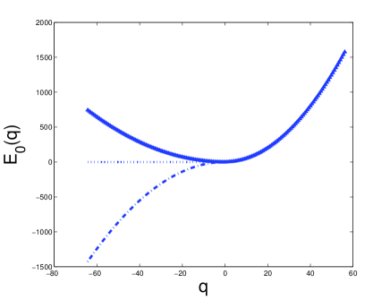
Figure 1: The lowest energy band in the single oscillator model for $\omega=1$ and $\alpha=0.8$ (upper, full line), $\alpha=1$ (middle, dotted line) and $\alpha=1.3$ (lower, dashed-dotted line).

II.4 Band dynamics: inverted oscillator.

An intuitive picture of the above results is provided by an approximate description of the dynamics, to be presented in this section. Hamiltonian (1) (with $L=2\pi$) may also be presented in the following form:

$${\cal H}\;=\;\int^{\oplus}_{{\mathbb{R}}}dq\;\mathrm{H}_{\alpha}(q)\;+\;{\mathbb{I}}\otimes H^{\mbox{\rm\tiny(osc)}}_{\omega}\;,$$ (31)

where, for any fixed value of $q$,

$$\mathrm{H}_{\alpha}(q)\;=\;H^{(p)}\;+\;\alpha q\;\delta(x)$$ (32)

is an operator in $L^{2}_{+}({\mathbb{S}})$ RS2 . It has a complete set of eigenfunctions and eigenvalues which parametrically depend on the product $\alpha q$. All eigenfunctions are real valued and have the form:

$$\phi_{q,n}(x)\;=\;A_{n}\;\cos(\xi_{n}(|x|-\pi))\;\;\,\;\;n=0,1,2,\ldots$$ (33)

where $A_{n}$ are normalization constants, and $\xi_{n}$ are the solutions with $\Re{\text{e}}(\xi)\geq 0$ of the equation:

$$\tan(\pi\xi)\;=\;\frac{\alpha q}{\xi}\;.$$

They are numbered in increasing order of the corresponding energy eigenvalues $W_{n}(q)=\tfrac{1}{2}\xi_{n}^{2}$. All $\xi_{n}$ with $n>0$ are real, and behave like $\xi_{n}\sim n+\tfrac{1}{2}$ asymptotically as $q\to\pm\infty$. Instead $\xi_{0}$ is real only when $q>0$, and turns imaginary when $q<0$ ; in that case $\xi_{0}=i\chi$, where $\chi$ is the unique positive solution of

$$\tanh(\pi\chi)\;=\;-\frac{\alpha q}{\chi}\;.$$

Hence $W_{0}(q)$ is negative whenever $q<0$. A standard Feynman-Hellman argument yields:

$$\frac{dW_{n}(q)}{dq}\;=\;\alpha\;\phi_{q,n}(0)^{2}\;,$$ (34)

so the levels $W_{n}(q)$ are nondecreasing functions of $q$. The ground state energy $W_{0}(q)$ is asymptotically given by:

$$W_{0}(q)\;=\;\tfrac{1}{2}\xi_{0}^{2}\;\sim\left\{\begin{array}[]{ll}\tfrac{1}{8},&\hbox{for\;$q\to+\infty$\;;}\\ -\tfrac{1}{2}\alpha^{2}q^{2},&\hbox{for\;$q\to-\infty$\;.}\end{array}\right.$$ (35)

When $q>0$, the ground state eigenfunction has still the form (33) with $n=0$. For $q<0$ it is instead given by:

$$\phi_{q,0}(x)\;=\;A_{0}\;\cosh\bigl{(}\chi(q)(|x|-\pi)\bigr{)}\;,\;\;\;(q<0)\;.$$

so for large negative $q$ it is sharply peaked at $x=0$. Any $\psi\in L^{2}_{+}({\mathbb{S}})\otimes L^{2}({\mathbb{R}})$ may be expanded as

$$\psi(x,q)\;=\;\sum\limits_{n=0}^{\infty}Q_{n}(q)\;\phi_{q,n}(x)\;\;,\;\;\;Q_{n}(q)=\int_{-\pi}^{\pi}dx\;\phi_{q,n}(x)\psi(x,q)\;,$$ (36)

so that

$$\sum\limits_{n=0}^{\infty}|Q_{n}(q)|^{2}\;=\;\int_{-\pi}^{\pi}dx\;|\psi(x,q)|^{2}\;.$$

In this way $\mathfrak{H}$ is decomposed in ”Band Subspaces” ${\mathfrak{B}}_{n}\equiv\{\psi(x,q)=Q_{n}(q)\phi_{q,n}(x)\;|\;Q_{n}(q)\in L^{2}({\mathbb{R}})\}$. The projector onto the $n$-th band subspace will be denoted $\Pi_{n}$. In the ”band formalism” it is easy to show that ${\cal H}_{\alpha,\omega}$ is bounded from below when $\alpha<\omega$. Indeed, if $\psi$ is in the domain of ${\cal H}_{\alpha,\omega}$, then

$$(\psi,{\cal H}_{\alpha,\omega}\psi)\; = \;\sum\limits_{n=0}^{\infty}\int_{-\infty}^{\infty}dq\;W_{n}(q)|Q_{n}(q)|^{2}\;+\;(\psi,{\mathbb{I}}\otimes H^{\mbox{\rm\tiny(osc)}}_{\omega}\psi)\;.$$ (37)

Singling out the contribution of the lowest band $\mathfrak{B}_{0}$, and using (35) and monotonicity of $W_{0}(q)$:

$$(\psi,{\cal H}_{\alpha,\omega}\psi) \geq \;-\frac{1}{2}\alpha^{2}\int_{-\infty}^{\infty}dq\;\int_{-\pi}^{\pi}dx\;q^{2}|\psi(x,q)|^{2}\;+$$ (38)

$$\;+\;\sum\limits_{n=1}^{\infty}\int_{-\infty}^{\infty}dq\;W_{n}(q)|Q_{n}(q)|^{2}\;+\;(\psi,{\mathbb{I}}\otimes H^{\mbox{\rm\tiny(osc)}}_{\omega}\;\psi)$$

$$\geq \;(\psi,{\mathbb{I}}\otimes H^{\mbox{\rm\tiny(osc)}}_{\sqrt{\omega^{2}-\alpha^{2}}}\psi)$$

$$\geq \;\frac{1}{2}\sqrt{\omega^{2}-\alpha^{2}}\;\|\psi\|^{2}\;.$$

This shows that the abrupt change from semibounded to unbounded spectrum which occurs at $\alpha=\omega$ is related to a change in the structure of the ”ground band” alone. This transition is further elucidated by noting that the ground band plays the role of a stable variety, due to the following:

Proposition 4

If $\alpha>\omega$ then, for arbitrary $\psi\in{\mathfrak{H}}_{\mbox{\tiny ac}}$, and for all integer $n>0$:

$$\lim\limits_{t\to\infty}\|\;\Pi_{n}e^{-i{\cal H}_{\alpha,\omega}t}\psi\;\|\;=\;0\;.$$

A proof is presented in section V.6. This suggests that asymptotic solutions in time of the time-dependent Schrödinger equation may be sought in the form $\psi(x,q,t)=Q_{0}(q,t)\phi_{q,0}(x)$. No exact proof is attempted here; nevertheless, direct substitution yields a Schrödinger equation for the band wavefunction $Q_{0}(q,t)$:

$$i\frac{\partial Q_{0}}{\partial t}\;=\;-\frac{1}{2}\frac{\partial^{2}Q_{0}}{\partial q^{2}}\;+\;{\cal V}(q)Q_{0}\;,$$

where the band potential ${\cal V}(q)$ is given by:

$${\cal V}(q)\;=\;\frac{1}{2}\omega^{2}q^{2}\;+\;W_{0}(q)\;+\;\frac{1}{2}\int_{{\mathbb{S}}}dx\;\biggl{|}\frac{\partial\phi_{q,0}(x)}{\partial q}\biggr{|}^{2}\;.$$ (39)

A calculation reported in Note V.7 shows that the last term on the right-hand side is $O(q^{-2})$ as $q\to-\infty$ and tends to a constant when $q\to+\infty$. At large $q$, the band potential is then determined by the other two terms. The band potential which results of these two terms alone is shown in Fig.1. As $\alpha$ grows beyond $\omega$, it turns from concave to monotone increasing and then, at large negative $q$, ${\cal V}(q)\sim-\frac{1}{2}(\alpha^{2}-\omega^{2})q^{2}$, that is the potential of an inverted harmonic oscillator. This sort of phase transition qualitatively explains the growth of the harmonic oscillator’s energy which was proven in Proposition 1, and suggests that it is exponential with rate $\lambda^{-1}=2\sqrt{\alpha^{2}-\omega^{2}}$.

III Collapse of wave-packets.

III.1 A multi-oscillator model.

Smilansky’s model has generalizations, in which an arbitrary finite number $N$ of harmonic oscillators interact with the particle at different points $O_{1},\ldots,O_{N}$ . In the $L=\infty$ case, the corresponding spectral theory has been developed by Evans and Solomyak ES05 using a scattering theory approach. Translated to the present case, this approach is as follows. All oscillators are assumed to have the same frequency $\omega$ and coupling constant $\alpha$, and a circular ordering is assumed for the interaction points $O_{i}$. For each $i=1,\ldots,N$ let a rigid wall be inserted at a point $Z_{i}$ in between $O_{i}$ ad $O_{i+1}$, and let $J_{i}$ denote the arc $Z_{i},Z_{i+1}$. The Hamiltonian ${\cal H}^{(b)}$ of the resulting system differs from ${\cal H}$ because of Dirichlet conditions at the points $Z_{i}$, and is actually an orthogonal sum of operators ${\cal H}^{(b)}_{i}$ in ${\mathfrak{H}}_{i}\equiv L^{2}(J_{i})\otimes L^{2}({\mathbb{R}}^{N})$, each of which describes the particle in a rigid box $J_{i}$, coupled to the $i$-th oscillator alone. Therefore, thanks to what is known about the single-oscillator box model, ${\cal H}^{(b)}$ has ac spectrum coinciding with ${\mathbb{R}}$ when $\alpha>\omega$. Møller wave operators are defined by :

$$\Omega_{\pm}({\cal H},{\cal H}^{(b)})\;=\;\lim\limits_{t\to\pm\infty}e^{i{\cal H}t}\;e^{-i{\cal H}^{(b)}t}\;P_{ac}^{(b)}$$ (40)

where $P_{ac}^{(b)}$ denotes projection onto the absolutely continuous subspace of ${\cal H}^{(b)}$. They are said to be complete if their range coincides with the entire absolutely continuous subspace of ${\cal H}$. Whenever this happens, the wave operators $\Omega_{\pm}({\cal H}^{(b)},{\cal H})$ also exist RS3 . Existence and completeness have been proven in ES05 for the model with $L=\infty$. Here they are assumed also for the multi-oscillator box model. In the absence of a formal proof paraphrasing Evans and Solomyak’s, this assumption rests on intuition provided by Proposition 2: as the wave function which evolves in ${\mathfrak{H}}_{i}$ under Hamiltonian ${\cal H}^{(b)}_{i}$ is drained by the $i$-th interaction point, the boundaries at $Z_{i}$ and $Z_{i+1}$ become ininfluent, and so does the difference between $\cal H$ and ${\cal H}^{(b)}$ .
Existence and completeness of wave operators enforce unitary equivalence of the absolutely continuous parts of $\cal H$ and of ${\cal H}^{(b)}$, hence infinitely degenerate Lebesgue spectrum of $\cal H$ at $\alpha>\omega$.

III.2 Band formalism.

There is a band formalism also for the N-oscillators case. The case $N=2$ will be briefly described. Oscillators $1$ and $2$ with respective coordinates $q_{1}$ and $q_{2}$ are coupled to the particle at points $x=0$ and $x=\pm\pi$ respectively, diametrally opposite in ${\mathbb{S}}$. The particle Hamiltonian which now replaces (32) parametrically depends on $q_{1}$ and $q_{2}$, and has real-valued eigenfunctions $\phi_{q_{1},q_{2},n}(x)$ in $L^{2}({\mathbb{S}}_{+})$ and eigenvalues $W_{n}(q_{1},q_{2})=\tfrac{1}{2}\xi_{n}^{2}$, where $\xi_{n}$ are the solutions with $\Re{\text{e}}(\xi_{n})\geq 0$ (numbered in non-decreasing order of the corresponding eigenvalues) ) of the equation:

$$\tan(\pi\xi)\;=\;\frac{\alpha\xi(q_{1}+q_{2})}{\xi^{2}-\alpha^{2}q_{1}q_{2}}.$$ (41)

”Band potentials” $E_{n}(q_{1},q_{2})=\tfrac{1}{2}\omega^{2}(q_{1}^{2}+q_{2}^{2})+W_{n}(q_{1},q_{2})$ computed by numerically solving eq. (41) are shown in Fig.2 and in Fig.3. Like in the $N=1$ case, the spectral transition at $\alpha=\omega$ is concomitant to a phase transition in the structure of the lowest band. A transition is observed for the 2nd lowest energy band as well, at a higher value of $\alpha/\omega\approx 1.414$ (not shown), but not for higher bands. The structure of the overcritical ground band, shown in Fig. 3, is explained as follows. When $1<\alpha/\omega$ , $\xi_{0}$ is found to be imaginary in the region $\mathcal{R}$ of the $(q_{1},q_{2})$ plane which is defined by the inequality:

$$q_{-}\;<\;-\frac{q_{+}}{1+\pi q_{+}}\;,$$

where $q_{-}$ and $q_{+}$ are respectively the minimum and the maximum of $q_{1}$ and $q_{2}$. Moving out to infinity in $\cal R$ along a half-line started at $(0,0)$, the asymptotic behaviour of $\xi_{0}$ is $\sim-i\alpha q_{-}$, so the band potential $E_{0}(q_{1},q_{2})$ diverges to $-\infty$, except along directions lying within an angle of $\arcsin(\omega/\alpha)-\pi/4$ on either side of the half-line $q_{1}=q_{2}<0$, where instead it diverges to $+\infty$ as long as $\omega<\alpha<\omega\sqrt{2}$. This is why in Fig.3 one observes two valleys , hereby labeled $1$ and $2$, that descend to $-\infty$ along the negative $q_{1}$ axis and the negative $q_{2}$ axis respectively, and are separated by a crest, which rises along the $q_{1}=q_{2}<0$ half-line. In region $\mathcal{R}$ the ground eigenfunction has the form

$$\phi_{q_{1},q_{2},0}(x)\;=\;C_{1}(q_{1},q_{2})\;e^{|\xi_{0}(q_{1},q_{2})||x|}\;+\;C_{2}(q_{1},q_{2})e^{-|\xi_{0}(q_{1},q_{2})||x|}\;.$$

It has two peaks, labeled $1$ and $2$, at the interaction points of oscillators $1$ and $2$. Descending along either valley both peaks become narrower and narrower, however calculation shows that the whole probability is asymptotically in time caught within the peak which shares the label of the valley.
Like in sec. II.4, for $\omega<\alpha<\omega\sqrt{2}$, the quantum dynamics is asymptotically attracted by the $0$-th band subspace, which consists of functions of the form $Q_{0}(q_{1},q_{2})\phi_{0,q_{1},q_{2}}(x)$. The ”band wave-function” $Q_{0}(q_{1},q_{2},t)$ asymptotically in time solves the Schrödinger equation for a particle in the plane $(q_{1},q_{2})$, subject to a potential that behaves at $\infty$ like the one in Fig. 3. A classical particle would escape to infinity along one valley, so one and just one oscillator would undergo unbounded excitation.

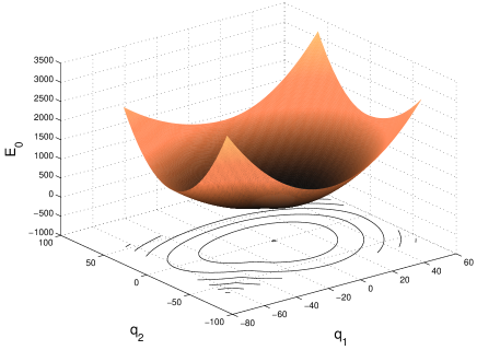
Figure 2: The lowest energy band in the model with 2 oscillators, for $\alpha=0.7$ and $\omega=1$.

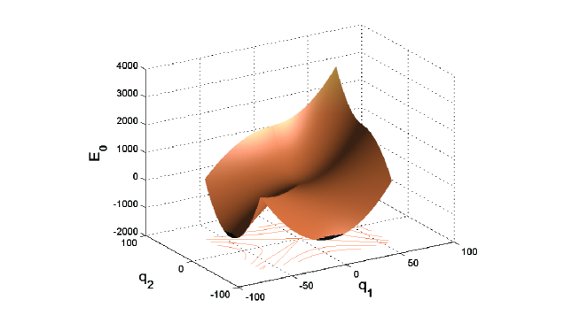
Figure 3: Same as Fig.2, for $\alpha=1.3$ and $\omega=1$.

III.3 Collapse of wave-packets.

Existence and completeness of wave operators have the following immediate consequence, which generalizes Proposition 3:

Proposition 5

If $\alpha>\omega$ and $\psi\in{\cal H}_{ac}$ with $\|\psi\|=1$, then the probability distribution of the particle converges weakly as $t\to\pm\infty$ to a superposition of $\delta$ functions supported in the interaction points.

$$\idotsint\limits_{{\mathbb{R}}^{N}}dq_{1}\ldots dq_{N}\;|\psi(x,q_{1},\ldots,q_{N},t)|^{2}\;\;\underset{t\to\pm\infty}{\longrightarrow}\;\;\sum\limits_{j=1}^{N}\gamma_{j}^{\pm}\;\delta(x-O_{j})\;,$$

where:

$$\gamma_{j}^{\pm}\;=\;\|P_{j}\;\Omega_{\pm}({\cal H}^{(b)},{\cal H})\psi\|^{2}\;,$$ (42)

and $P_{j}$ denotes projection onto ${\mathfrak{H}}_{j}$.

A proof is presented in section V.8. This in particular implies that the right-hand sides in (42) do not depend on the positions $Z_{i}$ of the rigid walls.
Corollary 1 about complete decoherence of the reduced state of the particle generalizes to the multi-oscillator case. Hence one may say that coupling to the oscillators causes the reduced state of the particle to evolve exponentially fast towards an ”incoherent superposition of position eigenstates”. In the case when the particle is initially in a pure state, this process is similar to the wave-packet reduction which is conventionally associated with measurements of position. Here the measuring apparatus consists of $N$ oscillators, and the $N$ interaction points have to be chosen in a thick homogeneous grid. Under the assumptions in Proposition 5, as $t\to+\infty$ the pure state $\psi(t)=e^{-i{\cal H}t}\psi$ comes closer and closer to the state $e^{-i{\cal H}^{(b)}t}\Omega^{+}\psi$. This is a coherent superposition of states which have the particle in a box and the corresponding oscillator in a highly excited state. Tracing out the oscillators yields an incoherent mixture of alternatives for the particle position , however the probability of finding the particle in the $m$-th box is given by $\gamma^{+}_{m}=\|P_{m}\Omega_{+}\psi\|^{2}$ as in eqn. (42) and not by $\int_{J_{m}}dx|\psi_{0}(x)|^{2}=\|P_{m}\psi\|^{2}$ as in an ideal measurement. The difference lies with replacing the initial state $\psi$ with the ”outgoing state” $\Omega_{+}\psi$ , and may be ascribed to the non-instantaneous nature of the measurement process. Increasing the number $N$ of oscillators (hence increasing the precision of the measurement) while keeping $\alpha/N$ and $\omega/N$ constant causes the time scale of the exponentially fast reduction process to decrease proportional to $1/N$ (see the scaling rule (3), and remarks in the end of sect.II.4). This suggests a possibility of retrieving the ideal measurement of position by a suitable limit process.

IV Concluding Remarks.

Dynamical instability in Smilansky’s model is due to a positive feedback loop between fall of the particle in the $\delta$- potential well and excitation of the oscillator. This effect may not crucially rest on point interaction, nor on linear dependence of the interaction on the coordinate of the oscillator. While such special features are probably optimal in simplifying mathematical analysis, a similar behavior may be reproducible with smoother interaction potentials and also in purely classical models.
Smilansky’s model is somewhat unrealistic from a physical viewpoint, as it is not easy to conceive of physical realizations, albeit approximate. Generalizations of the model to higher dimension, and more realistic couplings - if at all possible - may enhance physical interest.

Acknowledgment: I thank Uzy Smilansky for discussions about his model and Raffaele Carlone for making me aware of exact results in related fields.

V Notes, and proofs.

V.1 BA&WL Theory.

Corollary 2 to Proposition 6, which is proven in this Note, is an essential ingredient in the derivation of the spectral expansion in Sect. II.2 (notably in the proof of Lemma 1). Proposition 6 is proven by a rephrased version of a method which was introduced by Wong and Li WL92 in the context of a theory of Birkhoff and Adams about asymptotic expansions for $n\to+\infty$ of solutions of 2nd order difference equations of the form :

$$C(n+2)\;+\;p(n)\;C(n+1)\;+\;q(n)\;C(n)\;=\;0\;.$$ (43)

The main result of that theory (Theorem 8.36 in ref.El99 ) is that , whenever coefficients $p(n)$ and $q(n)$ have asymptotic expansions for $n\to\infty$ in powers of $n^{-1}$:

$$p(n)\;\sim\;\sum\limits_{k=0}^{+\infty}a(k)\;n^{-k}\;,\;\;\;q(n)\;\sim\;\sum\limits_{k=0}^{+\infty}b(k)\;n^{-k}\;,$$ (44)

the equation has two linearly independent ”normal” solutions, which have asymptotic expansions:

$$C_{\pm}^{\star}(n)\;\sim\;\sigma_{\pm}^{n}\;n^{\alpha_{\pm}}\;\sum\limits_{s=0}^{\infty}c_{\pm}(s)\;n^{-s}$$ (45)

where $\sigma_{\pm}$ are the (assumedly distinct) roots of the equation:

$$\sigma^{2}\;+\;a(0)\;\sigma\;+\;b(0)\;=\;0\;,$$ (46)

and

$$\alpha_{\pm}\;=\;\frac{a(1)\;\sigma_{\pm}\;+\;b(1)}{a(0)\;\sigma_{\pm}\;+\;2b(0)}\;.$$ (47)

Coefficients $c_{\pm}(s)$ in (45) are recursively determined by directly substituting (45) in (43) with $c_{\pm}(0)=1$. Eqn.(11) may be written in the form of eqn. (43), with coefficients that additionally depend on $E$:

$$p(n)\;=\;p(n,E)\;=\;-\;\frac{h_{1}(n,E)}{h_{2}(n,E)}\;,\;\;\;q(n)\;=\;q(n,E)\;=\;-\;\frac{h_{0}(n,E)}{h_{2}(n,E)}\;,$$ (48)

where $h_{0},\;h_{1},\;h_{2}$ are as in eqs. (13) and (14). Using (9) and (10) one computes asymptotic expansions (44). In particular,

$$a(0,E)\;=\;\tfrac{2\omega}{\alpha}\;,\;\;a(1,E)\;=\;-\tfrac{\omega}{\alpha}\bigl{(}1+\tfrac{E}{\omega}\bigr{)}\;,\;\;b(0,E)\;=\;1\;,\;\;b(1,E)\;=\;-1\;,$$

whence it follows that expansions (45) have the form (15) at lowest orders.
In the following $I$ will denote an arbitrary closed interval contained in ${\mathbb{R}}\setminus{\cal E}^{*}_{\omega}$; positive quantities only dependent on $\alpha,\omega,I$ will be denoted by $c_{1},c_{2},\ldots$; derivatives with respect to $E$ will be denoted by a dot, like, e.g., in $\dot{p}(n,E),\dot{q}(n,E)\ldots$. The following Lemma 2 sets premises for the proof of Proposition 6.

Lemma 2

For all positive $n$, $p(n,E)$ and $q(n,E)$ as given by (48), (13), (14) are $C^{1}$ functions of $E\in I$. Their asymptotic expansions (44) are uniform in $I$ . Their derivatives have uniform asymptotic expansions in $I$ in powers of $n^{-1}$, with coefficients given by the derivatives of the coefficients $a(s,E)$, $b(s,E)$, as specified in (48), (13), and (14). In particular, $n|\dot{p}(n,E)|$ and $n|\dot{q}(n,E)|$ are bounded in $I$ by some $c_{1}>0$.

Proof: by direct inspection. $\Box$

Proposition 6

For all $n\geq 0$ the normal solutions $C_{\pm}^{\star}(n,E)$ of eqn.(43), with coefficients as in (48), are $C^{1}$ functions of $E\in I$.

Proof: the proof is the same for both normal solutions, so suffixes $\pm$ will be left understood throughout. Thanks to Lemma 2, all coefficients $c(s,E)$ are $C^{1}$ functions of $E\in I$, because each of them is determined by a finite number of coefficients $a$ and $b$. Let $\mathfrak{R}$ and ${\mathfrak{R}}_{0}$ denote operators that act on sequences $w:{\mathbb{N}}\times{\mathbb{R}}\to{\mathbb{C}}$ according to

$$({\mathfrak{R}}w)(n,E)\;=\;w(n+2,E)\;+\;p(n,E)w(n+1,E)\;+\;q(n,E)w(n,E)\;,$$ (49)

$$({\mathfrak{R}}_{0}w)(n,E)\;=\;w(n+2,E)\;+\;a(0,E)w(n+1,E)\;+\;b(0,E)w(n,E)\;.$$ (50)

Let $Y(n,E)\;=\;\exp(\pm in\theta\mp i\lambda E\log(n))$, and let a normal solution be written in the form:

$$C^{\star}(n,E)=L_{N}(n,E)+\epsilon_{N}(n,E)\;,$$ (51)

where $N$ is an integer, and $L_{N}(n,E)$ is obtained on truncating at the $(N-1)$-th order the asymptotic expansion (45) of the normal solution:

$$L_{N}(n,E)=n^{-1/2}Y(n,E)\sum_{0}^{N-1}c(s,E)n^{-s}\;.$$

Direct calculation yields

$$({\mathfrak{R}}L_{N})(n,E)\;=\;n^{-1/2}\;Y(n,E)\;R_{N}(n,E)\;,$$ (52)

where , for any fixed $n$, $R_{N}(n,E)$ is a $C^{1}$ function of $E\in I$, because such are all coefficients $c(s,E)$, $(0\leq s\leq N-1)$; and, moreover,

$$R_{N}(n,E)=O(n^{-N-1})\;,$$ (53)

uniformly with respect to $E\in I$ as $n\to\infty$. Differentiating (52) on both sides, $\dot{R}_{N}(n,E)$ is found to have a uniform asymptotic expansion in $I$ in powers of $n^{-1}$, so (53) entails that

$$\dot{R}_{N}(n,E)=O(n^{-N-1})\;,$$ (54)

uniformly in $I$. Substitution of (51) and (52) into (43) yields:

$$({\mathfrak{R}}\epsilon_{N})(n,E)\;=\;-n^{-1/2}\;Y(n,E)\;R_{N}(n,E)\;,$$

which is equivalent to

$$({\mathfrak{R}}_{0}\epsilon_{N})(n,E)\;=\;-n^{-1/2}\;Y(n,E)\;R_{N}(n,E)\;-\;{\tilde{q}}(n,E)\epsilon_{N}(n,E)\;-\;{\tilde{p}}(n,E)\epsilon_{N}(n+1,E)\;,$$ (55)

where ${\tilde{p}}(n,E)=p(n,E)-a_{0}(E)$ and ${\tilde{q}}(n,E)=q(n,E)-b_{0}(E)$ . Eqn.(55) may be read as a inhomogeneous 2nd order difference equation, so it can be rewritten in ”integral” form using a ”Green function” for the operator ${\mathfrak{R}}_{0}$. This is provided by the function WL92 :

$$G(n)\;=\;s(n-1)\;\frac{\sin\bigl{(}(n-1)\theta\bigr{)}}{\sin(\theta)}$$ (56)

where $s(n)=1$ for $n\geq 0$, and $s(n)=0$ for $n<0$. Therefore, introducing the operator $\mathfrak{G}$ that formally acts on sequences as in:

$$({\mathfrak{G}}w)(n,E)\;=\;-\sum\limits_{k=n}^{+\infty}G(n-k)\;\bigl{(}{\tilde{q}}(k,E)\;w(k,E)\;+\;{\tilde{p}}(k,E)\;w(k+1,E)\bigr{)}\;,$$ (57)

and denoting

$$d_{N}(n,E)\;=\;-\sum\limits_{k=n}^{+\infty}G(n-k)\;k^{-1/2}Y(k,E)R_{N}(k,E)\;,$$ (58)

the sequence $\epsilon_{N}(n,E)$ must solve the following equation written in vector form :

$$\epsilon_{N}\;=\;d_{N}\;+\;{\mathfrak{G}}\;\epsilon_{N}\;.$$ (59)

No solution of the homogeneous equation ${\mathfrak{R}}_{0}\epsilon_{N}=0$ appears on the rhs of (59), because such solutions do not vanish at infinity, as is instead required of $\epsilon_{N}(n,E)$. Let $\sigma$ and $\sigma^{\dagger}$ denote the left shift operator and its adjoint: $(\sigma w)(n,E)=w(n+1,E)$, $(n\geq 1)$, $(\sigma^{\dagger}w)(n,E)=w(n-1,E)$ if $n>1$, and $(\sigma^{\dagger}w)(1,E)=0$. If $\epsilon_{N}$ satisfies (59), then ${\tilde{\epsilon}}_{N}:=\sigma^{N}\epsilon_{N}$ satisfies:

$${\tilde{\epsilon}}_{N}\;=\;\sigma^{N}d_{N}\;+\;{\mathfrak{G}}_{N}\;{\tilde{\epsilon}}_{N}\;,\;\;\;\;{\mathfrak{G}}_{N}\;=\;\sigma^{N}{\mathfrak{G}}\sigma^{\dagger N}\;.$$ (60)

The operator ${\mathfrak{G}}_{N}$ is explicitly given by eqn.(57) after replacing $\tilde{a}$, $\tilde{b}$ by $\sigma^{N}{\tilde{a}}$, $\sigma^{N}{\tilde{b}}$ respectively. Thanks to Lemma 3 and to the Contraction Mapping theorem, if $N$ is sufficiently large then eqn.(60) has a unique solution in the Banach space ${\mathfrak{X}}_{N,I}$ of sequences $w:{\mathbb{N}}\to C^{1}(I)$ such that

$$\|w\|_{\mathfrak{X}}\;:=\;\|w\|_{N}\;+\;\|\dot{w}\|_{N*}\;<\;+\infty\;,$$ (61)

where

$$\|w\|_{N}\;=\;\sup\;\{(N+n)^{N+1/2}|w(n,E)|\;,\;n\geq 0,\;E\in I\}\;,$$

$$\|w\|_{N^{*}}\;=\;\sup\;\biggl{\{}(N+n)^{N+1/2}\frac{1}{\log(N+n)}|w(n,E)|\;,\;n\geq 0,\;E\in I\biggr{\}}\;.$$ (62)

The thus found ${\tilde{\epsilon}}_{N}$ determines $\epsilon_{N}(n,E)$ as a $C^{1}$ function, and hence, via eqn.(51), the normal solution, for $n\geq N+1$. For such $n$ the thesis is then proven, because $L_{N}(n,E)$ is itself $C^{1}$ wrt $E$ thanks to already noted properties of coefficients $c(s,E)$. The values of the normal solution thus found at $n=N+1$ and $n=N+2$ can then be used to retrieve the normal solution for $0\leq n\leq N$ by solving eqn.(43) backwards (which is possible, because $q(n,E)\neq 0$ for all $n\geq 0$, thanks to the assumption that $E$ is not in ${\cal E}_{\omega}^{*}$). As this process involves a finite number of steps, and $p,q$ are $C^{1}$ functions, the proof is complete. $\Box$

Lemma 3

(i) $\sigma^{N}d_{N}\in{\mathfrak{X}}_{N,I}$, (ii) ${\mathfrak{G}}_{N}$ is a bounded operator in ${\mathfrak{X}}_{N,I}$, and its norm is bounded by:

$$\|{\mathfrak{G}}\|_{\mathfrak{X}}\;\leq\;2ec_{2}(c_{1}+3\beta)(N+1/2)^{-1}\;,$$

where $c_{1}$ is as in Lemma 2, $c_{2}=\sin(\theta)^{-1}=(1-\omega^{2}/\alpha^{2})^{-1/2}$, and

$$\beta\;=\;\sup\;\{k\;\bigl{(}|{\tilde{p}}(k,E)|\;+\;|{\tilde{q}}(k,E)|\;,\;k\in{\mathbb{N}},\;E\in I\bigr{\}}\;.$$

Proof: (i) from eqs.(58) and (53):

$$d_{N}(n,E)\;\leq\;c_{2}\sum\limits_{k=n}^{+\infty}k^{-N-3/2}\;=\;O(n^{-N-1/2})\;,$$

therefore $\|d_{N}\|_{N}$ is finite and so is $\|\sigma^{N+1}d_{N}\|_{N}$. Next, the derivative of the $k$-th term in the sum on the rhs in eqn.(58) is $O(k^{-N-3/2}\log(1+k))$, so the sum of such derivatives is absolutely and uniformly convergent in $I$ to the derivative of $d_{N}(n,E)$, and $\|\dot{d}_{N}\|_{N*}$ is finite.
(ii): noting that

$$\sup\{(k+N)\sigma^{N}\tilde{p}(k,E)\;|\;k\geq n\}\;\leq\;\beta\;,$$

and similarly for $\tilde{q}$, one may write:

$$\bigl{|}({\mathfrak{G}}_{N}w))(n,E)\bigr{|}\;\leq\;c_{2}\beta\|w\|_{N}\sum\limits_{k=n}^{+\infty}(N+k)^{-N-3/2}$$

$$\leq\;c_{2}\beta\|w\|_{N}\int_{n-1}^{+\infty}\;(N+x)^{-N-3/2}$$

$$=\;c_{2}\beta\|w\|_{N}(N+1/2)^{-1}(N+n-1)^{-N-1/2}\;,$$ (63)

so

$$\|{\mathfrak{G}}_{N}w\|_{N}\;\leq\;2c_{2}e\beta(N+1/2)^{-1}\|w\|_{N}$$ (64)

thanks to $(N+n)^{N+1/2}(N+n-1)^{-N-1/2}<2e$. To estimate $\|({\mathfrak{G}}_{N}w)^{\dot{}}\|_{N*}$:

$$({\mathfrak{G}}_{N}w)^{\dot{}}(n,E)\;\leq\;c_{2}c_{1}\|w\|_{N}\sum\limits_{k=n}^{+\infty}(k+N)^{-N-3/2}\;+\;$$

$$+\;c_{2}\beta\|\dot{w}\|_{N*}\sum\limits_{k=n}^{+\infty}(k+N)^{-N-3/2}{\log(k+N)}\;.$$ (65)

Estimating the sums on the rhs as it was done in (63) leads to:

$$\|({\mathfrak{G}}_{N}w)^{\dot{}}\|_{N*}\;\leq\;\bigl{(}2c_{1}c_{2}e\|w\|_{N}\;+\;4c_{2}e\beta\|\dot{w}\|_{N*}\bigr{)}(N+1/2)^{-1}\;.$$

Thanks to definition (61), the latter estimate along with (64) yield the claimed bound on the norm of ${\mathfrak{G}}_{N}$ as an operator in ${\mathfrak{X}}_{N,I}$. $\Box$

Corollary 2

If $E\in{\mathbb{R}}\setminus{\cal E}_{\omega}^{*}$ then the difference equation (11) has a particular solution which satisfies the initial condition (12), and moreover has the asymptotics (19), where $\zeta(E)$ is a $C^{1}$ function of $E$ in any closed interval of energies containing no exceptional points.

Proof: the complex amplitude $Z(E)$ (cp. eqn.(17)), which determines the sought for solution in terms of the normal solutions, is found by solving eqs.(18); so it is a smooth function of the values of the normal solutions at $n=0$ and $n=1$. The conclusion follows, because $\zeta(E)$ is the phase of $Z(E)$. $\Box$

V.2 Proof of Lemma 1.

First it will be proven that if $E^{m}\Psi(E)\in L^{2}({\mathbb{R}})$ for some integer $m$ then $\psi=\imath(\Psi)$ is in the domain of ${\cal H}^{m}$, and $\imath(E^{m}\Psi)={\cal H}^{m}{\psi}$.
It is easy to see that

$$L_{n}^{m}\psi_{n}(x)=c\int_{{\mathbb{R}}}dE\;\Psi(E)L^{m}_{n}u_{n}(x,E)=c\int_{{\mathbb{R}}}dE\;E^{m}\Psi(E)u_{n}(x,E)$$

(with $L_{n}$ defined as in (5)) holds for all $\Psi\in C_{0}({\mathbb{R}}\setminus{\cal E}_{\omega}^{*})$ and all positive integers $m,n$; so, thanks to (21) the sequence $\{L_{n}^{m}\psi_{n}\}_{n}$ is in $\ell^{2}({\mathbb{N}})\otimes L^{2}_{+}({\mathbb{S}})$ whenever $E^{m}\Psi(E)\in L^{2}({\mathbb{R}})$. On the other hand the sequence $\{L^{m}_{n}u_{n}\}_{n}$ satisfies the matching condition (6) because so does $u_{n}$, and because $L_{n}u_{n}=Eu_{n}$. The same is then true of the sequence $\{L^{m}_{n}\psi_{n}\}_{n}$, because the condition $\Psi\in C_{0}({\mathbb{R}}\setminus{\cal E}_{\omega}^{*})$ allows for computing left- and right-hand derivatives of $L^{m}\psi_{n}(x)$ at $x=0$ under the integral sign . Therefore $\psi$ is in the domain of ${\cal H}^{m}$ whenever $\Psi\in C_{0}({\mathbb{R}}\setminus{\cal E}_{\omega}^{*})$, and ${\cal H}^{m}\psi=\imath(E^{m}\Psi)$. As ${\cal H}^{m}$ is a closed operator, the same is true whenever $\Psi\in L^{2}({\mathbb{R}})$ and $E^{m}\Psi\in L^{2}({\mathbb{R}})$.
(ii) follows by continuity, because $\imath$ is isometric.
(iii) To prove that $\imath$ is onto: thanks to (21) and (28), the time-correlation $(\psi,e^{-i{\cal H}t}\psi)$ coincides with the Fourier transform of $|\Psi(E)|^{2}$. Therefore, $|\Psi(E)|^{2}$ is the density of the absolutely continuous spectral measure of $\psi$ with respect to ${\cal H}$ (also known as the local density of states). As ${\cal H}$ has a simple absolutely continuous spectrum coinciding with ${\mathbb{R}}$, $\psi$ is a cyclic vector whenever its local density of states is Lebesgue-almost everywhere different from zero. So, whenever $\Psi(E)$ is a.e. nonzero, $\psi$ is a cyclic vector of ${\cal H}$, so the closed span of $\{e^{-i{\cal H}t}{\psi}\}_{t\in{\mathbb{R}}}$ is the whole of $\ell^{2}({\mathbb{N}})\otimes L^{2}_{+}({\mathbb{S}})$, whence $\ell^{2}({\mathbb{N}})\otimes L^{2}_{+}({\mathbb{S}})=\imath(L^{2}({\mathbb{R}}))$ follows.

V.3 Proof of Proposition 2.

The expectation value of the energy of the oscillator in a state $\psi=\{\psi_{n}(x)\}\in\ell^{2}({\mathbb{N}})\otimes L^{2}_{+}({\mathbb{S}})$ of the composite system is given by:

$$\bigl{(}\psi,\mathbb{I}\otimes H^{\mbox{\rm\tiny(osc)}}_{\omega}\;\psi\bigr{)}\;=\;\sum\limits_{n=0}^{\infty}(n+\tfrac{1}{2})\omega\int_{-\pi}^{\pi}dx\;|\psi_{n}(x)|^{2}\;,$$

and so the sequence

$$P(n,E)\;:=\;\int_{-\pi}^{\pi}dx\;|u_{n}(x,E)|^{2}\;,\;\;\;(n\geq 0)\;,$$ (66)

may be thought of as a non-normalizable distribution of the energy of the oscillator over its unperturbed levels, when the full system has energy $E$. The present proof of Proposition 2 rests on the following inequality, which is an immediate consequence of eqs. (8),(9), (10), and (19):

$$\limsup\limits_{n\to+\infty}\;nP(n,E)\;\leq\;\pi^{-1}\;.$$ (67)

Let $\psi\in{\mathfrak{H}}_{\mbox{\rm\tiny ac}}$, $\|\psi\|=1$, and $\Psi(E)$ its spectral representative, so that $|\Psi(E)|^{2}$ is the density of the absolutely continuous spectral measure of $\psi$ with respect to ${\cal H}$. Thanks to (67) there is a continuous function $\Psi_{1}(E)$ , compactly supported in ${\mathbb{R}}\setminus{\cal E}_{\omega}^{*}$, so that on the one hand:

$$\int dE\;\bigl{|}\Psi(E)-\Psi_{1}(E)\bigr{|}^{2}<1/8\;,$$ (68)

and on the other hand :

$$\sum_{n=0}^{N}P(n,E)<C\ln(N)\;,\;\;\;\forall N\in{\mathbb{N}}\;$$ (69)

for some positive constant $C$ and for all $E$ in the support of $\Psi_{1}$. Let $\psi_{1}=\imath(\Psi_{1})$, $\psi_{2}=\psi-\psi_{1}$, and $\psi(t)=e^{-i{\cal H}t}\psi=\{\psi_{n}(x,t)\}\in\ell^{2}({\mathbb{N}})\otimes L^{2}_{+}({\mathbb{S}})$. For $T>0$ , the probability of finding the energy of the oscillator in its $n$-th level, averaged from time $0$ to time $T$, is:

$$p_{n}(T)=\frac{1}{T}\int_{0}^{T}dt\;\int_{-\pi}^{\pi}dx\;|\psi_{n}(x,t)|^{2}\;.$$ (70)

Let $p_{1,n}(T)$ and $p_{2,n}(T)$ denote the functions which are defined by the same equation, with $\psi$ replaced by $\psi_{1}$ and $\psi_{2}$ respectively. By construction of $\Psi_{1}$, the spectral representation of $\psi_{1}$ has the form (27), so Proposition 1 yields:

$$p_{1,n}(T)\;=\;\frac{1}{T}\int_{0}^{T}dt\;\int_{-\pi}^{\pi}dx\;\biggl{|}\int dE\;e^{-iEt}\Psi_{1}(E)\;u_{n}(x,E)\biggr{|}^{2}\;,$$ (71)

On the other hand, denoting $\cal{F}[.]$ the Fourier-Plancherel transform in $L^{2}({\mathbb{R}})$:

$$\int_{0}^{T}dt\;\biggl{|}\int dE\;e^{-iEt}\Psi_{1}(E)\;u_{n}(x,E)\biggr{|}^{2}\;=\;2\pi\int_{0}^{T}dt\;\bigl{|}{\cal F}\bigl{[}\Psi_{1}\;u_{n}(x,.)\bigr{]}(t)\bigr{|}^{2}$$ (72)

$$\leq\;2\pi\|{\cal F}\bigl{[}\Psi_{1}\;u_{n}(x,.)\bigr{]}\|^{2}\;=\;2\pi\|\Psi_{1}\;u_{n}(x,.)\|^{2}$$ (73)

$$=\;2\pi\int dE\;u_{n}^{2}(x,E)|\Psi_{1}(E)|^{2}\;.$$ (74)

Replacing (74) in (71), and using (66) and inequality (69), which holds throughout the support of $\Psi_{1}$ :

$$\sum\limits_{n=0}^{N}p_{1,n}(T)\;\leq\;2\pi CT^{-1}\ln(N)\;.$$ (75)

With $N=N(T):=e^{C_{1}T}$, where $C_{1}=1/(16\pi C)$, this estimate yields:

$$\sum\limits_{n\leq N_{T}}p_{1,n}(T)\;<\;\tfrac{1}{8}.$$ (76)

From the definitions of $p_{n}(T),p_{1,n}(T),p_{2,n}(T)$, and ineq. (18) it immediately follows that:

$$\sum\limits_{n=0}^{N(T)}p_{n}(T)\;\leq\;2\sum\limits_{n=0}^{N(T)}p_{1,n}(T)\;+\;2\sum\limits_{n=0}^{N(T)}p_{2,n}(T)\;<\;\tfrac{1}{4}\;+\;\tfrac{1}{4}\;=\;\tfrac{1}{2}\;,$$

and so

$$\frac{1}{T}\int_{0}^{T}dt\;\bigl{(}\psi(t),\mathbb{I}\otimes H^{\mbox{\rm\tiny(osc)}}_{\omega}\;\psi(t)\bigr{)}\;>\;\bigl{(}\tfrac{1}{2}\;+\;N(T)\bigr{)}\omega\sum\limits_{n>N(T)}p_{n}(T)\;>\;\tfrac{1}{2}N(T)\omega\;=\;\tfrac{1}{2}e^{C_{1}T}\omega\;.$$ (77)

V.4 Proof of Proposition 3.

For $0<\eta<\pi$ let $A_{\eta}=(-\pi,-\eta)\cup(\eta,\pi)$. The explicit form of $u_{n}$ given in eqs.(8) and (9) shows that $|u_{n}(x)|\leq|C(n,E)|\rho_{n}\cosh(\chi_{n}(E)(\pi-\eta))$, whenever $n>E/\omega-1/2$ and $x\in A_{\eta}$; so, if in addition $E\in{\mathbb{R}}\setminus{\cal E}_{\omega}^{*}$, then from (10) and from the asymptotic formula (19) it follows that

$$\sum\limits_{0}^{+\infty}\int_{A_{\eta}}dx\;u_{n}^{2}(x,E)\;<\;+\infty\;.$$ (78)

because the integrals in the sum decrease exponentially fast for $n\to\infty$. Thanks to (78), for $0<\epsilon<1$ one can find a compact set $B_{\epsilon}\subset{\mathbb{R}}\setminus{\cal E}_{\omega}^{*}$ and a continuous function $\Psi_{\epsilon}$ supported in $B_{\epsilon}$, so that, on the one hand:

$$\sum\limits_{0}^{+\infty}\int_{A_{\eta}}dx\;u_{n}^{2}(x,E)\;<\;C_{\epsilon}\;,\;\;\;\forall E\in B_{\epsilon}\;,$$ (79)

for some positive constant $C_{\epsilon}$; and, on the other hand, $\|\psi-\psi^{(\epsilon)}\|^{2}<\epsilon$, where $\psi^{(\epsilon)}=\imath(\Psi_{\epsilon})$. Then:

$$\iint\limits_{A_{\eta}\times{\mathbb{R}}}dx\;dq\;|\psi(x,q,t)|^{2}\;\leq\;2\iint\limits_{A_{\eta}\times{\mathbb{R}}}\;|\psi(x,q,t)-\psi^{(\epsilon)}(x,q,t)|^{2}\;+$$

$$+\;2\iint\limits_{A_{\eta}\times{\mathbb{R}}}dx\;dq\;|\psi^{(\epsilon)}(x,q,t)|^{2}$$

$$\leq\;2\|\psi-\psi^{(\epsilon)}\|^{2}\;+\;2\iint\limits_{A_{\eta}\times{\mathbb{R}}}dx\;dq\;|\psi^{(\epsilon)}(x,q,t)|^{2}$$

$$\leq\;2\epsilon\;+\;2\iint\limits_{A_{\eta}\times{\mathbb{R}}}dx\;dq\;|\psi^{(\epsilon)}(x,q,t)|^{2}\;.$$ (80)

From eqn.(4):

$$\iint\limits_{A_{\eta}\times{\mathbb{R}}}dx\;dq\;|\psi^{(\epsilon)}(x,q,t)|^{2}\;=\;\sum\limits_{n=0}^{+\infty}\int_{A_{\eta}}dx\;|\psi^{(\epsilon)}_{n}(x,t)|^{2}\;,$$

and then, since the spectral representative $\Psi_{\epsilon}$ of $\psi^{(\epsilon)}$ is compactly supported in ${\mathbb{R}}\setminus{\cal E}_{\omega}^{*}$, the spectral representation (27) can be used to the effect that:

$$\iint\limits_{A_{\eta}\times{\mathbb{R}}}dx\;dq\;|\psi^{(\epsilon)}(x,q,t)|^{2}\;=\;\iint\limits_{B_{\epsilon}\times B_{\epsilon}}dE\;dE^{\prime}\;e^{-i(E^{\prime}-E)t}\;\;\overline{\Psi_{\epsilon}(E)}\Psi_{\epsilon}(E^{\prime})\;G_{\eta}(E,E^{\prime})\;,$$ (81)

where :

$$G_{\eta}(E,E^{\prime})\;=\;\int_{A_{\eta}}dx\;\sum\limits_{n=0}^{+\infty}\;u_{n}(x,E)u_{n}(x,E^{\prime})\;.$$

Thanks to (79), $G_{\eta}(E,E^{\prime})$ is bounded in $B_{\epsilon}\times B_{\epsilon}$; on the other hand $\Psi_{\epsilon}(E)$ is summable over $B_{\epsilon}$, so the integral on the rhs in (81) tends to $0$ in the limit $t\to\infty$ thanks to the Riemann-Lebesgue lemma. From (80) it follows that

$$\limsup\limits_{t\to\infty}\iint\limits_{A_{\eta}\times{\mathbb{R}}}dx\;dq\;|\psi(x,q,t)|^{2}\;\leq\;2\epsilon\;,$$

whence the claim (30) follows, because $\epsilon>0$ is arbitrary.

V.5 Proof of Corollary 1.

By positivity of $S(t)$, it is sufficient to prove the claim for $\phi=\phi^{\prime}$ and $\|\phi\|=1$. Let $P_{\phi}=(\phi,.)\phi$ denote projection along $\phi$, and let $P_{\eta}$, $P^{\bot}_{\eta}$ respectively denote projection onto the functions supported in $\eta<|x|<\pi$, and its orthogonal complement. Then:

$$(\phi,S(t)\phi)\;=\;\mbox{\rm Tr}(S(t)P_{\phi})\;\leq\;|\mbox{\rm Tr}(S(t)P_{\phi}P_{\eta})|\;+\;|\mbox{\rm Tr}(S(t)P_{\phi}P^{\bot}_{\eta})|\;.$$ (82)

For any $\eta>0$ the 1st term on the rhs in (82) tends to $0$ as $t\to\pm\infty$ thanks to eqn.(30), due to

$$|\mbox{\rm Tr}(S(t)P_{\phi}P_{\eta})|\;=\;|\bigl{(}\psi(t),P_{\phi}P_{\eta}\otimes{\mathbb{I}}\;\psi(t)\bigr{)}|\;\leq\;\|P_{\eta}\otimes{\mathbb{I}}\;\psi(t)\|\;.$$

On the other hand, the 2nd term on the rhs in (82) can be made arbitrarily small, uniformly with respect to $t$, by choosing $\eta$ small enough:

$$|\mbox{\rm Tr}(S(t)P_{\phi}P^{\bot}_{\eta})|\;\leq\;\|P_{\phi}P^{\bot}_{\eta}\|\;\leq\;\|P_{\eta}^{\bot}\phi\|\;,$$

Hence the lhs in (82), which does not depend on $\eta$, tends to $0$ in the limit $t\to\pm\infty$.

V.6 Proof of Proposition 4.

$$\int_{{\mathbb{R}}}dq\;|Q_{n}(q,t)|^{2}\;=\;\int_{{\mathbb{R}}}dq\;\biggl{|}\biggl{(}\int_{|x|<\eta}+\int_{\eta<|x|<\pi}\biggr{)}dx\;\phi_{q,n}(x)\psi(x,q,t)\biggr{|}^{2}$$

$$\leq\;\int_{{\mathbb{R}}}dq\;\bigl{\{}R(\eta,q)\;+\;S(\eta,q)\bigr{\}}$$ (83)

where:

$$R(\eta,q)\; = \;2\;\biggl{|}\int_{|x|<\eta}dx\;\phi_{q,n}(x)\psi(x,q,t)\biggr{|}^{2}$$

$$S(\eta,q)\; = \;2\;\biggl{|}\int_{\eta<|x|<\pi}dx\;\phi_{q,n}(x)\psi(x,q,t)\biggr{|}^{2}$$ (84)

From the Cauchy-Schwarz inequality:

$$\int_{{\mathbb{R}}}dq\;R(\eta,q)\;\leq\;2\int_{{\mathbb{R}}}dq\biggl{(}\int_{|x|<\eta}dx\;\phi^{2}_{q,n}(x)\biggr{)}\biggl{(}\int_{|x|<\eta}dx\;|\psi(x,q,t)|^{2}\biggr{)}\;,$$ (85)

and using that $\phi_{q,n}$ with $n>0$ are uniformly bounded (by $(\pi-1)^{-1/2}$) and that $\|\psi(t)\|=1$,

$$\int_{{\mathbb{R}}}dq\;R(\eta,q)\;\leq\;C\eta\;,$$

for a suitable constant $C$. Similarly, using Cauchy-Schwarz and $\int dx\phi_{q,n}^{2}(x)=1$,

$$\int_{{\mathbb{R}}}dq\;S(\eta,q)\;\leq\;\int_{{\mathbb{R}}}dq\int_{\eta<|x|<\pi}dx\;|\psi(x,q,t)|^{2}\;,$$

so, thanks to Proposition 3,

$$\limsup\limits_{t\to\infty}\int_{{\mathbb{R}}}dq\;|Q_{n}(q,t)|^{2}\;\leq\;C\eta\;,$$

and the claim follows because $\eta>0$ is arbitrary. $\Box$
The above argument fails if $n=0$, because $\phi_{q,0}$ is not uniformly bounded in $q<0$.

V.7 About the Band potential.

Here the 3d term in the band potential (39) is estimated. A standard perturbative calculation yields:

$$\gamma_{nl}(q)\;\equiv\;\int_{{\mathbb{S}}}dx\;\phi_{q,n}(x)\frac{\partial\phi_{q,l}(x)}{\partial q}\;=\;\alpha\;\frac{\phi_{q,n}(0)\phi_{q,l}(0)}{W_{l}(q)-W_{n}(q)}\;,\;\;\;(n\neq l)$$ (86)

and $\gamma_{nn}=0$; so, thanks to orthonormality and completeness of $\{\phi_{q,n}\}$:

$$\int_{{\mathbb{S}}}dx\;\biggl{(}\frac{\partial\phi_{q,0}}{\partial q}\biggr{)}^{2}\;=\;\sum\limits_{n=1}^{+\infty}\gamma_{n0}^{2}(q)$$ (87)

$$=\;\alpha^{2}\phi_{q,0}^{2}(0)\sum\limits_{n=1}^{+\infty}\frac{\phi_{q,n}^{2}(0)}{(W_{n}(q)-W_{0}(q))^{2}}\;.$$ (88)

It is easy to see that $|\phi_{q,n}(0)|\leq(\pi-1)^{-1/2}$ whenever $n>0$, that $W_{n}(q)>\tfrac{1}{2}n^{2}$, and that $|\phi_{q,0}|\sim\sqrt{-\alpha q}$ for $q\to-\infty$. Using this and the asymptotic form of $W_{0}(q)$ given in (35), (87) is found to be $O(q^{-2})$ for $q\to-\infty$ and $\sim$const. as $q\to+\infty$.

V.8 Proof of Proposition 5.

The following notations will be used. For sufficiently small $\eta>0$, $A_{j,\eta}=J_{j}\setminus D_{j}$ where $D_{j}\subset J_{j}$ is an arc of size $\eta>0$ centered at $O_{j}$; and $A_{\eta}=\cup_{j}A_{j,\eta}$. $P_{\eta}$ will denote the projector of $L^{2}({\mathbb{S}})\otimes L^{2}({\mathbb{R}}^{N})$ onto $L^{2}(A_{\eta})\otimes L^{2}({\mathbb{R}}^{N})$, and $P_{j,\eta}$ will denote the projector of $L^{2}(J_{j})\otimes L^{2}({\mathbb{R}}^{N})$ onto $L^{2}(A_{j,\eta})\otimes L^{2}({\mathbb{R}}^{N})$.
Existence of $\Omega_{\pm}\equiv\Omega_{\pm}({\cal H}^{(b)},{\cal H})$ entails that:

$$\lim\limits_{t\to\pm\infty}(e^{-i{\cal H}t}\psi\;,P_{\eta}\;e^{-i{\cal H}t}\psi)\;=\;\lim\limits_{t\to\pm\infty}(e^{-i{\cal H}^{(b)}t}\Omega_{\pm}\psi\;,P_{\eta}\;e^{-i{\cal H}^{(b)}t}\Omega_{\pm}\psi)$$

$$=\;\lim\limits_{t\to\pm\infty}\sum\limits_{j=1}^{N}(e^{-i{\cal H}^{(b)}t}\Omega_{\pm}\psi\;,P_{j,\eta}\;e^{-i{\cal H}^{(b)}t}\Omega_{\pm}\psi)\;.$$ (89)

The quantity of which the $t\to\infty$ limit is taken in the above equations is the probability of finding the particle in $A_{\eta}$ at time $t$. Each subspace $P_{j}({\mathfrak{H}})$ is invariant under the evolution ruled by ${\cal H}^{(b)}$, so the sum in the last line is equal to

$$\sum\limits_{j=1}^{N}(e^{-i{\cal H}^{(b)}t}P_{j}\Omega_{\pm}\psi\;,P_{j,\eta}\;e^{-i{\cal H}^{(b)}t}P_{j}\Omega_{\pm}\psi)\;.$$ (90)

Each term in the sum is a probability of finding the particle at time $t$ in $J_{j,\eta}$ with the evolution $e^{-i{\cal H}^{(b)}t}$. In each invariant subspace this evolution is that of a single-oscillator model, so, thanks to Proposition 3, each term in the sum tends to $0$ as $t\to\infty$. Hence, so does the probability of finding the particle in $A_{\eta}$ for all $\eta>0$, which is equivalent to the thesis. $\Box$

References

- (1) U.Smilansky, Irreversible Quantum Graphs, Waves in Random Media 14 (2004) 143.
- (2) M.Solomyak, On a differential operator appearing in the theory of irreversible quantum graphs, Waves in Random Media 14 (2004) 173.
- (3) S.N.Naboko, M.Solomyak, On the absolutely continuous spectrum in a model of an irreversible quantum graph, Proc. London Math. Soc. (3) 92 (2006) 251.
- (4) W.D.Evans, M.Solomyak, Smilansky’s model of irreversible quantum graphs: I. The absolutely continuous spectrum J.Phys A (Math. Gen.) 38 (2005) 4611.
- (5) C.Cacciapuoti, R.Carlone, and R.Figari, A solvable model of a Tracking Chamber, Rep. Math. Phys. 59 (2007) 337.
- (6) C.Cacciapuoti, R. Carlone, and R.Figari, Decoherence induced by scattering: a three-dimensional model, J. Phys. A (Math. Gen.) 38 (2005) 4933.
- (7) G.Dell’Antonio, R.Figari, and A.Teta, Joint excitation probability for two harmonic oscillators in one dimension and the Mott problem, J. Math. Phys. 49 (2008) 042105.
- (8) K. Hornberger, J.E. Sipe, Collisional Decoherence reexamined, Phys. Rev. A 68, (2003) 012105.
- (9) A. Kiselev, Y.Last, Solutions, spectrum, and dynamics for Schrödinger operators on infinite domains, Duke Math. J. Volume 102, 1 (2000), 125-15.
- (10) A.Erdélyi, W. Magnus, F. Oberhettinger, F. Tricomi, Higher transcendental functions. Vol. II, McGraw-Hill (1955), p.207.
- (11) M.Reed and B.Simon, in Methods of Modern Mathematical Physics vol.II, Academic Press, San Diego, CA 1975, p.168 example 3.
- (12) M.Reed and B.Simon, in Methods of Modern Mathematical Physics vol.III, Academic Press, San Diego, CA 1975.
- (13) S.N.Elaydi, An introduction to Difference Equations, Springer New York 1999.
- (14) R.Wong and H.Li, Asymptotic expansions for second-order difference equations, J. Comp. Appl. Math. 41 (1992) 65.