On the Energy Dependence of the Dipole-Proton Cross Section in Deep Inelastic Scattering

Abstract:

We study the dipole picture of high-energy virtual-photon-proton scattering. It is shown that different choices for the energy variable in the dipole cross section used in the literature are not related to each other by simple arguments equating the typical dipole size and the inverse photon virtuality, contrary to what is often stated. We argue that the good quality of fits to structure functions that use Bjorken-$x$ as the energy variable – which is strictly speaking not justified in the dipole picture – can instead be understood as a consequence of the sign of scaling violations that occur for increasing $Q^{2}$ at fixed small $x$. We show that the dipole formula for massless quarks has the structure of a convolution. From this we obtain derivative relations between the structure function $F_{2}$ at large and small $Q^{2}$ and the dipole-proton cross section at small and large dipole size $r$, respectively.

1 Introduction

The colour dipole model [1, 2, 3] provides a successful description of deep inelastic scattering (DIS) processes in a wide range of the kinematic variables. We consider here electron- and positron-proton scattering,

$$e^{\pm}+p\to e^{\pm}+X\,,$$ (1)

at not too high momentum transfers squared $Q^{2}$, $Q^{2}\lesssim 1000~{}\mbox{GeV}^{2}$ say, and at high energies. There, only the exchange of a virtual photon $\gamma^{*}$ between the leptons and the hadrons has to be taken into account. Thus, we study in essence the absorption of a high-energy virtual photon on a proton,

$$\gamma^{\ast}+p\rightarrow X\,.$$ (2)

The structure functions for this inclusive DIS process were extensively measured at HERA [4, 5, 6, 7, 8, 9]. A considerable part of the literature concerning the proton structure functions in DIS uses the colour dipole picture as an essential input. In particular, the interpretation of the structure function $F_{2}$ at small Bjorken-$x$ relies heavily on the dipole picture. The corresponding results are frequently used in the context of various scattering processes in proton-proton collisions at the LHC and in the description of the initial conditions of the creation of the quark-gluon plasma in heavy-ion collisions. Also calculations for processes at a future lepton-hadron collider [10] are often based on the dipole picture. Obviously, a good understanding of the dipole picture and its consequences is very important for all these applications. In the present study we shall consider an aspect of the dipole picture that has – in our opinion – not yet received proper attention in the literature, namely the correct choice of energy variable in the dipole-proton cross section.

The idea that the high energy photon in the reaction (2) acts in some way like a hadron goes back a long time. It has been used for instance since the 1960s in vector dominance models, see [11, 12] for reviews. Today, the dipole picture is frequently used in analyses of DIS structure functions. There, the reaction (2) is viewed as a two-step process. In the first step the photon splits into a quark-antiquark pair which represents the colour dipole. Subsequently, that pair scatters on the proton, this second step being a purely hadronic reaction. For reviews we refer the reader to [13, 14]. In [15, 16] the foundations of this dipole picture were examined in detail. The precise assumptions which have to be made in order to arrive at it were spelled out. In [17, 18] it was shown that already the general formulae of the standard dipole approach allow one to derive stringent bounds on various ratios of structure functions. These bounds were used to determine the kinematic region where the dipole picture is possibly applicable. In particular, it was found that for $\gamma^{\ast}p$ c. m. energies $W$ in the range 60 to 240 GeV the standard dipole picture fails to be compatible with the HERA data for $Q^{2}$ larger than about $100$ to $200$ GeV², see Fig. 9 of [18].

The derivations of some of these bounds rely on the dipole-proton cross sections $\hat{\sigma}^{(q)}$, where $q$ denotes the quark flavour, being independent of $Q^{2}$. In [16] it has been stressed that this $Q^{2}$-independence of the dipole-proton cross section is in fact natural. The correct energy variable is given exclusively by $W$ and the functional dependence of $\hat{\sigma}^{(q)}$ should be

$$\hat{\sigma}^{(q)}=\hat{\sigma}^{(q)}(r,W)\,,$$ (3)

where $r$ is the transverse size of the dipole. This excludes in particular the choice of Bjorken-$x$ instead of $W$, since this would introduce a dependence on $Q^{2}$ in addition to $W$, see (2) below. In the derivation [15, 16] of the dipole picture the dipole cross section arises from a $T$-matrix element for the scattering of a dipole state on the proton. The key feature of these dipole states is that they consist of a quark and an antiquark described by asymptotic states. The dipole states are then independent of $Q^{2}$ in the high energy limit. Upon a smearing in the relative transverse vector $\boldsymbol{r}$ between quark and antiquark and in the longitudinal momentum fraction $\alpha$ of the photon carried by the quark the dipole states can be viewed as hadron analogues, whose normalisation is independent of continuous internal degrees of freedom. But also the mean squared invariant mass of such smeared dipole states is independent of $Q^{2}$ at large $W$. Since any physical cross section can depend only on variables defined by the incoming states, the dipole-proton cross section hence cannot depend on $Q^{2}$. Nevertheless, the energy variable $x$ – and therefore a $Q^{2}$-dependence – is frequently used in popular models for the dipole cross section, such as [19]. Further examples for $x$-dependent dipole cross sections are [20], [21], and [22]. Sometimes also other dependencies on $Q^{2}$ are introduced by modifying the photon wave functions [23, 24]. Other models introduce an impact parameter dependence of the dipole cross section, see [25, 26]. For an overview of the physical motivations for various models see for instance [27]. Furthermore, the perturbative gluon density $g(x,Q^{2})$ naturally depends on $x$ and $Q^{2}$ and its often assumed proportionality to the dipole cross section suggests that the latter is also $Q^{2}$-dependent. A subtle point in such a comparison is given by the fact that different limits are used for the dipole picture and the double leading logarithmic approximation, respectively, see the discussion in [16]. Only very few models for the dipole cross section have been constructed that use the correct functional dependence (3), among them are [24], [28], and [29].

Through the interplay of photon wave function and dipole cross section a typical transverse dipole size is generated, which depends on $Q$. In this paper we shall investigate whether such an effective dipole size can be used to relate different choices of energy variables in the dipole cross section.

We consider then the dipole formulae for the case of massless quarks and show that these formulae can be understood as a convolution. This is used to analyse the relation of the structure functions and the dipole cross section. For high and for low $Q^{2}$ we find simple but somewhat surprising relations.

Our paper is organised as follows. Section 2 reviews the relevant formulae of the dipole picture. In section 3 we discuss typical dipole sizes and investigate whether different choices for the energy dependence of the dipole cross section may be related to each other by effective scale arguments. In section 4 we rewrite the dipole formula for massless quarks as a convolution. We present considerations suggesting that the success of using Bjorken-$x$ as the energy variable in the dipole cross section is due to the specific form of scaling violations in the structure function $F_{2}$. We derive asymptotic relations for the general dipole picture in the regimes of large and small $Q^{2}$, respectively. Our conclusions are drawn in section 5. Two appendices contain results used in the main text: In appendix A we derive the asymptotic behaviour of the integrated photon densities. Appendix B explains the steps for obtaining a simplified version of a $W$-dependent model for the dipole-proton cross section from the original model [29].

2 The dipole picture

We use the standard formulae for the kinematics and for the definitions of structure functions of the reaction (1), see for instance [30]. As discussed above, we consider $Q^{2}\lesssim 1000~{}\text{GeV}^{2}$ so that it is sufficient to take into account the exchange of a photon. Thus, we shall study in the following the absorption of a virtual photon $\gamma^{\ast}$ on the proton,

$$\gamma^{\ast}(q)+p(p)\rightarrow X(p^{\prime})\,.$$ (4)

Here the $4$-momenta are indicated in brackets. The c. m. energy for this reaction is denoted by $W$, the virtuality of $\gamma^{\ast}$ by $Q^{2}$. For these and the other usual variables we have

$$W^{2} =(p+q)^{2}\,,$$

$$Q^{2} =-q^{2}\,,$$

$$\nu =\frac{p\cdot q}{2m_{p}}\,,$$

$$x =\frac{Q^{2}}{2m_{p}\nu}=\frac{Q^{2}}{W^{2}+Q^{2}-m_{p}^{2}}\,.$$ (5)

The proton in (4) is supposed to be unpolarised, while the virtual photon can have transverse or longitudinal polarisation. The corresponding total cross sections are $\sigma_{T}(W,Q^{2})$ and $\sigma_{L}(W,Q^{2})$, respectively. The $F_{2}$ structure function is, with Hand’s convention [31] for the $\gamma^{\ast}$ flux factor,

$$F_{2}(W,Q^{2})=\frac{Q^{2}}{4\pi^{2}\alpha_{\rm em}}\left[\sigma_{T}(W,Q^{2})+\sigma_{L}(W,Q^{2})\right](1-x)+\mathcal{O}\left(\frac{m_{p}^{2}}{W^{2}}\right)\,.$$ (6)

For small Bjorken-$x$, $x\ll 1$, this simplifies to

$$F_{2}(W,Q^{2})=\frac{Q^{2}}{4\pi^{2}\alpha_{\mathrm{em}}}\left[\sigma_{T}(W,Q^{2})+\sigma_{L}(W,Q^{2})\right]\,.$$ (7)

In the following we shall use this simpler relation since we shall only consider the region $x\ll 1$.

In order to obtain the standard dipole model for the cross sections $\sigma_{T,L}$ we can relate them first to the imaginary part of the $\gamma^{\ast}p\to\gamma^{\ast}p$ forward scattering amplitude. The latter is represented as the initial $\gamma^{\ast}$ splitting into a $q\bar{q}$ pair, this pair scattering on the proton and the $q\bar{q}$ subsequently fusing into the final state $\gamma^{\ast}$, see Figure 1.

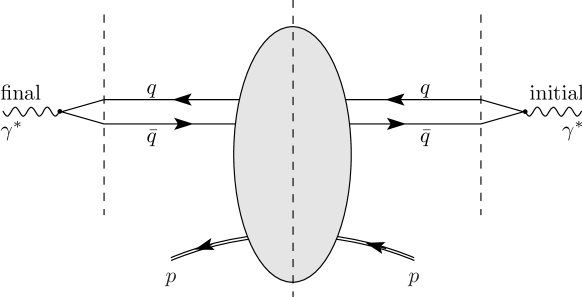
Figure 1: Basic diagram for the description of the cross sections $\sigma_{T,L}$ of $\gamma^{\ast}p$ scattering in the standard dipole approach.

With the assumptions spelled out in detail in section 6 of [16] the diagram of Figure 1 gives in the high energy limit

$$\sigma_{T,L}(W,Q^{2})=\sum_{q}\int\mathrm{d}^{2}r\,w^{(q)}_{T,L}(r,Q^{2})\,\hat{\sigma}^{(q)}(r,W)\,.$$ (8)

Here the integrated ‘photon densities’ are

$$w^{(q)}_{T}(r,Q^{2}) =\sum_{\lambda,\lambda^{\prime}}\int^{1}_{0}\mathrm{d}\alpha\,\left|\psi^{(q)+}_{\lambda\lambda^{\prime}}(\alpha,r,Q)\right|^{2}\,,$$ (9)

$$w^{(q)}_{L}(r,Q^{2}) =\sum_{\lambda,\lambda^{\prime}}\int^{1}_{0}\mathrm{d}\alpha\,\left|\psi^{(q)L}_{\lambda\lambda^{\prime}}(\alpha,r,Q)\right|^{2}\,.$$ (10)

We recall that $\alpha$ is the longitudinal momentum fraction of the $\gamma^{\ast}$ carried by the quark, $\boldsymbol{r}$ is the vector in transverse position space from the antiquark to the quark, $r=|\boldsymbol{r}|$, and $\lambda$ and $\lambda^{\prime}$ are the helicities of $q$ and $\bar{q}$, respectively. The total cross section for the scattering of the $q\bar{q}$ pair on the proton is denoted by $\hat{\sigma}^{(q)}$, the $\gamma^{\ast}$ wave functions for transversely and longitudinally polarised $\gamma^{\ast}$ by $\psi_{\lambda\lambda^{\prime}}^{(q)\,\pm}$ and $\psi_{\lambda\lambda^{\prime}}^{(q)\,L}$, respectively. A sum over all contributing quark flavours $q$ is to be performed in (8). Inserting in (9) and (10) the photon wave functions in leading order of $\alpha_{s}$ and assuming the longitudinal momenta of quark and antiquark to be much larger than their mass and transverse momenta we get the standard expressions

$$\sum_{\lambda,\lambda^{\prime}}\left|\psi_{\lambda\lambda^{\prime}}^{(q)+}(\alpha,\boldsymbol{r},Q)\right|^{2} =\frac{N_{c}}{2\pi^{2}}\,\alpha_{\rm em}Q_{q}^{2}\left\{\left[\alpha^{2}+(1-\alpha)^{2}\right]\epsilon_{q}^{2}[K_{1}(\epsilon_{q}r)]^{2}+m_{q}^{2}[K_{0}(\epsilon_{q}r)]^{2}\right\}\,,$$ (11)

$$\sum_{\lambda,\lambda^{\prime}}\left|\psi_{\lambda\lambda^{\prime}}^{(q)L}(\alpha,\boldsymbol{r},Q)\right|^{2} =\frac{2N_{c}}{\pi^{2}}\,\alpha_{\rm em}Q_{q}^{2}Q^{2}[\alpha(1-\alpha)]^{2}[K_{0}(\epsilon_{q}r)]^{2}\,.$$ (12)

Here $N_{c}=3$ is the number of colours, $Q_{q}$ is the charge of the quark in units of the proton charge, $K_{0,1}$ are modified Bessel functions, and

$$\epsilon_{q}=\sqrt{\alpha(1-\alpha)Q^{2}+m_{q}^{2}}\,.$$ (13)

For massless quarks $q$ the integrated photon densities $w^{(q)}_{T,L}$ of (9) and (10) can be calculated analytically. The corresponding formulae are given in appendix A.

In (8) we have written $\sigma_{T}$ and $\sigma_{L}$ as functions of $W$ and $Q^{2}$, and the dipole cross sections $\hat{\sigma}^{(q)}$ as functions of $r$ and $W$. It is one purpose of this paper to examine the consequences of choosing energy variables other than $W$ in the dipole formulae. Choosing, for instance, Bjorken-$x$ as variable we get again the formulae (8) but with $W$ everywhere replaced by $x$. On the l.h.s. of (8) this means, of course, just another and equivalent pair of variables. But for the r.h.s. this has drastic consequences as we shall show in the following.

3 Energy dependence of the dipole cross section

3.1 Typical dipole sizes

In [16] it was shown that in a formulation starting from the functional integral the dipole cross section $\hat{\sigma}^{(q)}$ comes out as independent of $Q^{2}$ and depends on $r$ and the energy $W$ only. We already noted that in contrast to this, prominent dipole models discussed in the literature introduce a dependence of $\hat{\sigma}^{(q)}$ on $Q^{2}$, typically through the Bjorken-$x$ variable. Often it is argued that in the dipole model one has a relation of the kind

$$r=\frac{C}{Q}\,,$$ (14)

with a constant $C$, corresponding to a ‘typical dipole size’ or ‘typical scale’. That is, the most relevant dipole sizes $r$ are determined by the scale $Q$. The reasoning behind this is the fact that due to the interplay of the $Q^{2}$-dependence of the photon wave function and the $r$-dependence of the dipole cross section a typical size is generated. Neglecting the $W$-dependence, the masses and all non-perturbative intrinsic scales, the typical size must be given by (14) for dimensional reasons. Taking (14) seriously one might be tempted to replace freely in $\hat{\sigma}(r,W)$ or related quantities $r$ by $Q^{2}$ dependencies and vice versa. In this section we shall show that such replacements are far from harmless and, in fact, are not admissible.

Let us first see how the relation (14) for typical dipole sizes arises. Inserting (8) into (7) we can write the dipole model expression for the structure function $F_{2}$ as

$$F_{2}(W,Q^{2})=Q\int_{0}^{\infty}\mathrm{d}r\sum_{q}h(Qr,m_{q}r)\,\frac{1}{r^{2}}\,Q_{q}^{2}\hat{\sigma}^{(q)}(r,W)\,.$$ (15)

Here we define

$$h(Qr,m_{q}r)=\frac{Qr^{3}}{2\pi\alpha_{\mathrm{em}}Q_{q}^{2}}\,\left[w_{T}^{(q)}(r,Q^{2})+w_{L}^{(q)}(r,Q^{2})\right]\,.$$ (16)

The dependence of the dimensionless functions $Qr^{3}w^{(q)}_{T,L}/(\alpha_{\rm em}Q_{q}^{2})$ on $r$, as resulting from (9)-(12), is shown in Figure 2 for the case of massless quarks.

Figure 2: Dependence of the dimensionless quantity $Qr^{3}w^{(q)}_{T,L}/(\alpha_{\rm em}Q_{q}^{2})$ on $r$ for massless ($q=u,d,s$) quarks for three different values $Q^{2}=1,10,100\,\mbox{GeV}^{2}$; on the left for transversely polarised photons, on the right for longitudinally polarised photons.

The function $h$ is shown in Figure 3. For massless quarks, $m_{q}=0$, $h$ is only a function of the dimensionless variable

$$z=Qr\,.$$ (17)

The function $h(z,0)$ has its maximum at

$$z_{0}=2.4010\,.$$ (18)

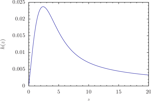
Figure 3: The function $h(z,0)$ defined in (16).

The behaviour of $h(z,0)$ for small and large $z$ is

$$\begin{split}&h(z,0)\propto z\quad\quad\quad\>\mbox{for}\>\>z\to 0\,,\\ &h(z,0)\propto\frac{1}{z}\quad\quad\quad\mbox{for}\>\>z\to\infty\,.\end{split}$$ (19)

In many proposed models colour transparency at small $r$ is implemented by assuming $\hat{\sigma}^{(q)}(r)\propto r^{2}$ for $r\to 0$. For larger $r$, on the other hand, the dipole cross sections are certainly not expected to grow faster than $r^{2}$. Thus $Q_{q}^{2}\hat{\sigma}^{(q)}(r)/r^{2}$ should be a rather smooth function of $r$. Let us now, for the sake of argument, consider massless quarks only. Then we get from (15)

$$F_{2}(W,Q^{2})=Q\int_{0}^{\infty}\mathrm{d}r\,h(Qr,0)\,f\left(r,\frac{1}{r^{2}W^{2}}\right)\,,$$ (20)

where we define the function $f$ by

$$\sum_{q}Q_{q}^{2}\hat{\sigma}^{(q)}(r,W)=r^{2}f\left(r,\frac{1}{r^{2}W^{2}}\right)\,.$$ (21)

In (20) a smooth function of $r$, $f(r,1/(r^{2}W^{2}))$, is integrated with $h(Qr,0)$ having a maximum at $r_{\textrm{max}}=z_{0}/Q$. It is now tempting to replace $r$ in the smooth function $f(r,1/(r^{2}W^{2}))$ by $r_{\textrm{max}}$. In this way we get a modified $F_{2}$,

$$F_{2}^{\mathrm{mod}^{\prime}}(W,Q^{2})=Q\int_{0}^{\infty}\mathrm{d}r\,h(Qr,0)\,f\left(\frac{z_{0}}{Q},\frac{x}{z_{0}^{2}}\right)\,,$$ (22)

where we used $Q^{2}/W^{2}\approx x$ for $W^{2}\gg Q^{2}$. By this trick the effective dipole cross section got a $Q^{2}$-dependence.

Of course, this is too simplistic and does not work since the integral in (22) diverges at large $r$ due to (19). But we can modify the above argument slightly and replace $r$ by $r_{\textrm{max}}=z_{0}/Q$ only where $r$ is associated with the energy scale $W$. In this way we get

$$F_{2}^{\mathrm{mod}}(W,Q^{2})=Q\int_{0}^{\infty}\mathrm{d}r\,h(Qr,0)\,f\left(r,\frac{x}{z_{0}^{2}}\right)\,.$$ (23)

Now the integral is in general convergent and we obtain a dipole formula with a dipole-proton cross section depending on $r$ and $x$. That is, we made the replacement of scales (14)

$$\sum_{q}Q_{q}^{2}\hat{\sigma}^{(q)}(r,W)\>\>\longrightarrow\>\>r^{2}f\left(r,\frac{x}{C^{2}}\right)\equiv\hat{\sigma}^{\mathrm{mod}}(r,x)$$ (24)

with $C=z_{0}=2.40$. But also other values of $C$ can be envisaged.

We now show that also the replacement (24) is far from harmless and, in fact, modifies the structure function in an essential way. Basically this is due to the fact that the function $h(z,0)$ is very broad and is not well approximated by a delta function at $z_{0}$.

3.2 Substitution of scales via typical dipole sizes: examples

We first consider an example where a $Q^{2}$-dependence is introduced via the ‘typical dipole size’ into a dipole cross section that originally depends only on $r$ and $W$ but not on $Q^{2}$. Actually there are only few examples for dipole models of the latter kind in the literature. We choose here a slightly simplified version of a model proposed by Donnachie and Dosch in [29]. This DD model is based on Regge theory and includes exchanges of a soft and a hard pomeron. The intercepts of the soft and hard pomeron trajectories are denoted by $(1+\epsilon_{s})$ and $(1+\epsilon_{h})$, respectively. The dipole cross section that we want to consider is

$$\hat{\sigma}^{(q)}_{\text{DD}}(r,W)=A_{0}r\left[1-\exp\left(-\frac{r}{3.1a}\right)\right]\left[\theta(R_{c}-r)\left(\frac{rW}{R_{c}W_{0}}\right)^{2\epsilon_{h}}+\theta(r-R_{c})\left(\frac{W}{W_{0}}\right)^{2\epsilon_{s}}\right]\,.$$ (25)

The parameter values are

$$\epsilon_{h} =0.42\,, A_{0} =57.4\,\mathrm{mb}/\mathrm{fm}\,, R_{c} =0.22\,\mathrm{fm}\,,$$

$$\epsilon_{s} =0.08\,, W_{0} =20\,\text{GeV}\,, a =0.346\,\mathrm{fm}\,.$$ (26)

We take into account only light quarks ($u,d,s$) and set their masses to zero for simplicity. In appendix B we show how this simplified model is obtained from the original, more general approach of [29]. Depending on the kinematic parameters the simplifications lead to non-negligible deviations from the original model. But the simplified version is sufficient for the sake of our argument even if it describes the data only moderately well in some kinematic region. We should point out that both the simplified and the original model exhibit a rather strong rise of $F_{2}$ at very small $x$ and large $Q^{2}$ that originates from the assumed high intercept of the hard pomeron in this model. However, substantial deviations from the Golec-Biernat-Wüsthoff model (see below) occur only in regions in which no data are available.

For the DD model we hence have

$$\hat{\sigma}_{\text{DD}}(r,W)=\sum_{q}Q_{q}^{2}\hat{\sigma}^{(q)}_{\text{DD}}(r,W)=r^{2}f_{\mathrm{DD}}\left(r,\frac{1}{r^{2}W^{2}}\right)\,,$$ (27)

where the sum is over the light flavours only and

$$\begin{split}f_{\mathrm{DD}}\left(r,\frac{1}{r^{2}W^{2}}\right)=&\sum_{q}Q_{q}^{2}\,A_{0}\,\frac{1}{r}\,\left[1-\exp\left(-\frac{r}{3.1a}\right)\right]\\ &\times\left[\theta(R_{c}-r)\left(\frac{r^{2}W^{2}}{R_{c}^{2}W_{0}^{2}}\right)^{\epsilon_{h}}+\theta(r-R_{c})\left(\frac{r^{2}W^{2}}{r^{2}W_{0}^{2}}\right)^{\epsilon_{s}}\right]\,.\end{split}$$ (28)

Making the replacement of scales (24) in (28) gives

$$\hat{\sigma}_{\mathrm{DD}}^{\mathrm{mod}}(r,x)=r^{2}f_{\mathrm{DD}}\left(r,\frac{x}{C^{2}}\right)$$ (29)

with $C=z_{0}=2.40$. As discussed above, this replacement changes the cross section only via terms which are sensitive to the external scale $W$, that is the terms in brackets with exponents $\epsilon_{h}$ and $\epsilon_{s}$ in this case. Figure 4 shows the effect of this substitution on the structure function $F_{2}$ obtained from these dipole cross sections (calculated only with light flavours). The solid curves show $F_{2}$ obtained using the (original) $W$-dependent dipole cross section $\hat{\sigma}_{\text{DD}}(r,W)$, while the dashed curves show $F_{2}$ calculated using the $x$-dependent $\hat{\sigma}_{\text{DD}}^{\text{mod}}(r,x)$. The results clearly deviate from each other. In particular, the $x$- and $Q^{2}$-dependences are heavily altered. This is also the case when one uses in the replacement of scales (14) not $C=z_{0}$ but $C=2z_{0}=4.80$, corresponding to larger ‘typical dipole sizes’. $F_{2}$ obtained with this latter replacement is shown as the dotted curves in Figure 4.

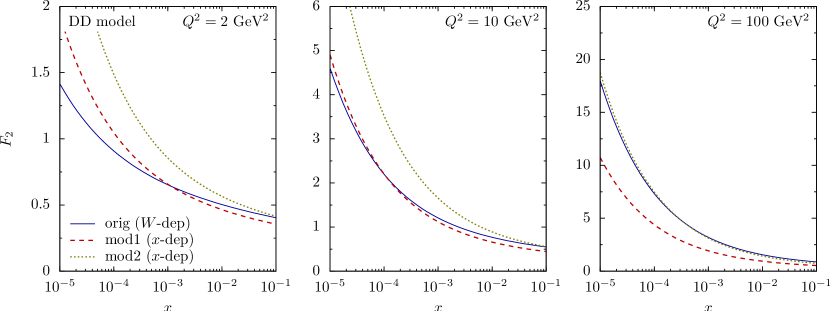
Figure 4: $F_{2}$ obtained from the simplified DD model for $\hat{\sigma}$ and modified versions thereof, with energy dependencies via ‘typical dipole size’ substitutions, for three values of $Q^{2}=2,10,100\,\mbox{GeV}^{2}$. Bjorken-$x$ is varied and $Q^{2}$ is kept fixed for each plot. Shown are the DD model with original $W$-dependence (solid curves) and modifications of type (24) with $C=z_{0}=2.40$ (‘mod1’, dashed curves) and $C=2z_{0}=4.80$ (‘mod2’, dotted curves).

Let us now consider the reverse substitution of scales. That is, let us start from an $x$-dependent dipole cross section $\hat{\sigma}(r,x)$ and make the reverse replacement of (24), namely

$$\hat{\sigma}(r,x)\equiv r^{2}f\left(r,\frac{x}{C^{2}}\right)\>\>\longrightarrow\>\>r^{2}f\left(r,\frac{1}{r^{2}W^{2}}\right)\equiv\hat{\sigma}^{\mathrm{mod}}(r,W)$$ (30)

with $C=z_{0}=2.40$. As an example we consider the dipole model proposed by Golec-Biernat and Wüsthoff [19]. This GBW model describes the $F_{2}$ data from HERA quite well. The dipole cross section of this model is given by

$$\hat{\sigma}_{\mathrm{GBW}}(r,x)=\sum_{q}Q_{q}^{2}\hat{\sigma}_{\mathrm{GBW}}^{(q)}(r,x)=\sum_{q}Q_{q}^{2}\sigma_{0}\left[1-\exp\left(-\left(\frac{r}{2R_{0}(x)}\right)^{2}\right)\right]\,.$$ (31)

Accordingly, we have

$$f_{\mathrm{GBW}}\left(r,\frac{x}{C^{2}}\right)=\frac{1}{r^{2}}\sum_{q}Q_{q}^{2}\sigma_{0}\left[1-\exp\left(-\left(\frac{r}{2R_{0}(x)}\right)^{2}\right)\right]\,.$$ (32)

For simplicity we consider also here only light ($u,d,s$) quarks, neglect their masses, and choose the following parameter set of [19]:

$$\begin{split}R_{0}(x)=\left(\frac{x}{x_{0}}\right)^{\lambda/2}\mbox{GeV}^{-1}\,\,,\>\>\>\>\>\sigma_{0}=23\,\mbox{mb},\>\>\>\>\>\lambda=0.29\,,\>\>\>\>\>x_{0}=3\cdot 10^{-4}\,.\end{split}$$ (33)

The replacement (30) gives us a modified dipole cross section $\hat{\sigma}_{\mathrm{GBW}}^{\mathrm{mod}}(r,W)$. Figure 5 shows the effect of this replacement on $F_{2}$. The curves for $F_{2}$ of the original GBW model (solid lines) are significantly modified by the substitution (30) (dashed lines), in particular the dependence on $Q^{2}$ and $x$ is altered. Again, this is also the case when using in the replacement of scales (14) not $C=z_{0}$ but $C=2z_{0}=4.80$, corresponding to larger ‘typical dipole sizes’, see the dotted lines in Figure 5.

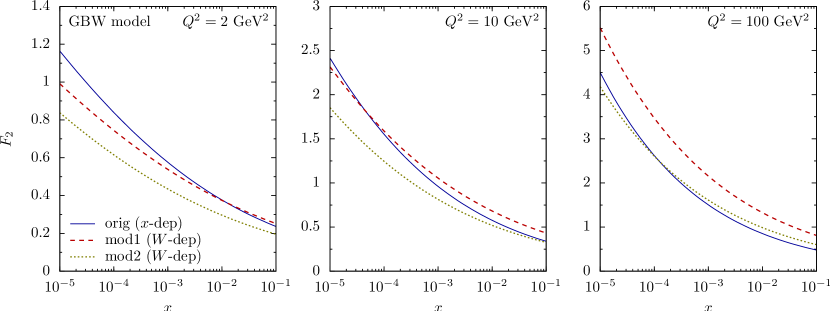
Figure 5: $F_{2}$ obtained from the GBW model for $\hat{\sigma}$ and modified versions thereof, with energy dependencies via ‘typical dipole size’ substitutions, for three values of $Q^{2}=2,10,100\,\mbox{GeV}^{2}$. Bjorken-$x$ is varied and $Q^{2}$ is kept fixed for each plot. Shown are the GBW model with original $x$-dependence (solid curves) and modifications of type (30) with $C=z_{0}=2.40$ (‘mod1’, dashed curves) and $C=2z_{0}=4.80$ (‘mod2’, dotted curves).

In this section we have shown on two examples that the substitution of scales $r\leftrightarrow C/Q$ (14) in the dipole cross section $\hat{\sigma}$, done in either way, alters the structure function $F_{2}$ significantly. As could have been expected, the direction of the alteration is opposite in the two directions of performing the substitution. (Clearly, if one applies the substitution and its reverse subsequently on the same dipole cross section $\hat{\sigma}$, the individual alterations have to cancel. The effect persists if one applies the two ways of substituting to different models which individually describe the data well.) The size of the alteration due to the substitution of scales is significant both quantitatively and qualitatively, see Figures 4 and 5.

Actually, we can infer already from the results of [17, 18] that the choice of the energy variable in $\hat{\sigma}$ is crucial at least at high $Q^{2}$. There it was shown that any dipole cross section of the form $\hat{\sigma}(r,W)$ fails to describe the HERA data for $Q^{2}>100$ to $200\,\mbox{GeV}^{2}$. In contrast, the GBW model with $\hat{\sigma}_{\text{GBW}}(r,x)$ provides a good fit to the data also at higher $Q^{2}$. From this we see that a dependence of $\hat{\sigma}$ on $Q^{2}$ in addition to $W$ can certainly not be eliminated or introduced by an effective scale argument of the type (14) in the regime of high $Q^{2}$ without drastic consequences. Let us, indeed, compare ratios of $F_{2}$ for different values of $Q^{2}$ for the models, original and modified, discussed above. An illustration of such ratios is given in Figure 6 for the example $W=150\,\mbox{GeV}$, where in addition the general bound (10) of [17] is shown, which is valid for any $\hat{\sigma}(r,W)$. We see that, as expected, $\hat{\sigma}_{\text{GBW}}^{\text{mod}}(r,W)$ as well as $\hat{\sigma}_{\text{DD}}(r,W)$ respect the general bounds. In contrast, the bounds are violated for both $x$-dependent cross sections $\hat{\sigma}_{\text{GBW}}(r,x)$ and $\hat{\sigma}_{\text{DD}}^{\text{mod}}(r,x)$.

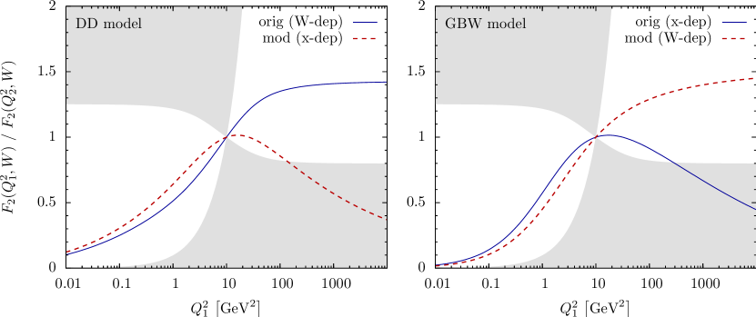
Figure 6: Ratio $F_{2}(W,Q_{1}^{2})/F_{2}(W,Q_{2}^{2})$ for two dipole models and modified versions with altered energy dependencies via ‘typical dipole size’ substitutions, for $W=150\,\mbox{GeV}$. Here, $Q_{1}^{2}$ is varied and $Q_{2}^{2}=10\,\mbox{GeV}^{2}$ is kept fixed. Left plot for the (simplified) $W$-dependent Donnachie-Dosch model (solid curve) and its modification (24) with $C=z_{0}=2.40$ (dashed curve). Right plot for the original Golec-Biernat-Wüsthoff model (solid curve) and its modification using (30) with $C=z_{0}=2.4$ (dashed curve). Quark masses are set to zero in all cases. The shaded area is excluded by the bound (10) of [17] for any $Q^{2}$-independent dipole cross section $\hat{\sigma}^{(q)}(r,W)$.

4 The dipole formula as a convolution

In this section we consider again, for simplicity, only the light quarks $u$, $d$, $s$ and neglect their masses. Our starting point is the relation (20) with $f$ inserted from (21). But now we leave the choice of energy variable open,

$$F_{2}(\xi,Q^{2})=Q\int_{0}^{\infty}\mathrm{d}r\,h(Qr,0)\,\frac{1}{r^{2}}\,\hat{\sigma}(r,\xi)\,,\qquad\hat{\sigma}(r,\xi)=\sum_{q}Q_{q}^{2}\hat{\sigma}^{(q)}(r,\xi)\,.$$ (34)

We recall that the function $h(Qr,0)$ is obtained directly from the photon wave functions, see (16). Here we set $\xi=W$ if we want to consider a $W$-dependent dipole cross section and $\xi=x$ for a $x$-dependent one. Correspondingly, we consider $F_{2}$ as function of $\xi$ and $Q^{2}$.

Now we show that (34) is a convolution formula. For this we set, as in (17), $Qr=z$ and define (recall that $z_{0}$ is defined as the position of the maximum of $h(z,0)$)

$$\tau =\ln(z/z_{0})\,,$$ (35)

$$\kappa(\tau) =z_{0}h(z_{0}e^{\tau},0)\,.$$ (36)

We have $0\leq z<\infty$ and $-\infty<\tau<\infty$. Corresponding to the behaviour of $h(z,0)$ for small and large $z$, see (19), we have

$$\kappa(\tau)\propto\exp(\pm\tau)\qquad\quad\text{for }\tau\to\mp\infty\,.$$ (37)

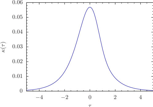
Figure 7: The function $\kappa(\tau)$ defined in (36).

The function $\kappa(\tau)$ is shown in Figure 7. The half width of this function is $\Delta\tau=2.22$. Now we choose $Q_{0}$ and $r_{0}$ such that

$$Q_{0}r_{0}=z_{0}$$ (38)

and define new variables, replacing $Q$ and $r$,

$$t=\ln(Q/Q_{0})$$ (39)

and

$$t^{\prime}=-\ln(r/r_{0})\,.$$ (40)

Furthermore, let us define a rescaled and reparametrised ‘dipole cross section’

$$S(\xi,t^{\prime})=\left.\frac{1}{rr_{0}}\,\hat{\sigma}(r,\xi)\right|_{r=r_{0}\exp(-t^{\prime})}\,.$$ (41)

The dipole formula for massless quarks (34) has now the form of a convolution

$$F_{2}(\xi,Q_{0}^{2}e^{2t})e^{-t}=\int_{-\infty}^{\infty}\mathrm{d}t^{\prime}\,\kappa(t-t^{\prime})S(\xi,t^{\prime})\,.$$ (42)

For dipole cross sections which are reasonably behaved for small and large $r$ the integral in (42) is convergent. Indeed, we find

$$S(\xi,t^{\prime})\propto\exp(-t^{\prime})\qquad\text{for }t^{\prime}\to\infty,\quad\text{if }\hat{\sigma}(r,\xi)\propto r^{2}\>\text{ for }\>r\to 0$$ (43)

and

$$S(\xi,t^{\prime})\propto\exp[(1-a)t^{\prime}]\qquad\text{for }t^{\prime}\to-\infty,\quad\text{if }\hat{\sigma}(r,\xi)\propto r^{a}\>\text{ for }\>r\to\infty\,.$$ (44)

In the following we shall assume $a<1$. That is, we assume that $\hat{\sigma}(r,\xi)$ increases more slowly than linearly with $r$ at large $r$. In many models the dipole cross section saturates for large $r$ which corresponds to $a=0$ in (44). With these assumptions the function $S(\xi,t^{\prime})$ decreases exponentially for $t^{\prime}\to\pm\infty$ and so does $\kappa(t-t^{\prime})$. Thus, the convolution formula (42) is well convergent.

We assume now, for the sake of the argument, that for some given $\xi$ the dipole formula (34) is valid for all $Q^{2}$, that is, (42) holds for all $t$. This allows us to draw some general conclusions:

1. The convolution formula (42) by itself places really no restrictions on $F_{2}$. We can, in principle, invert the formula, using well known techniques from the theory of integral transforms, and obtain $S(\xi,t^{\prime})$ and the dipole cross section from $F_{2}$. However, inversion is in general difficult and may constitute an ill-posed problem depending on the detailed structure of the functions involved. The physical restrictions enter in (42) from the requirement of a non-negative dipole cross section, that is, from

   $$S(\xi,t^{\prime})\geq 0\qquad\text{for all }t^{\prime}\,.$$ (45)

   Suppose now that we have indeed inverted the convolution (42) and found a non-negative $S(\xi,t^{\prime})$. Then the dipole-proton cross section $\hat{\sigma}(r,\xi)$ will appear as an integral over $Q^{2}$ of $F_{2}(\xi,Q^{2})$, respectively $\sigma_{T}(\xi,Q^{2})+\sigma_{L}(\xi,Q^{2})$, using (7). Setting now $\xi=x$ we would find that $\hat{\sigma}(r,x)$ is related to the $\gamma^{\ast}p$ cross sections at the same $x$ and all $Q^{2}$. This means that the dipole cross section at some fixed $r$ and $x$ would appear as (inverse) convolution of the structure function $F_{2}(x,Q^{2})$ at the same fixed $x$ but varying $Q^{2}$ corresponding to very different hadronic final states $X$ in (4). Taken literally, the final states would range from the single proton ($Q^{2}=0$) to multi-particle final states with arbitrarily high invariant mass for $Q^{2}\to\infty$. This looks not so plausible to us from the physics point of view. On the other hand, setting $\xi=W$, only $\gamma^{\ast}p$ cross sections for final states with the same c. m. energy will appear in the integral for $\hat{\sigma}(r,W)$. This appears much more plausible to us.

2. The function $\kappa(t-t^{\prime})$ in (42) is rather broad and decreases as $\exp(-t)$ for $t\to\infty$, see (37) and Figure 7. Superposing $\kappa(t-t^{\prime})$ with non-negative weights $S(\xi,t^{\prime})$ will lead to an even broader function of $t$ on the l.h.s. of (42). That is, the decrease of $F_{2}(\xi,Q_{0}^{2}e^{2t})\exp(-t)$ can then not be faster than $\exp(-t)$ for $t\to\infty$. This means that the dipole formula will be in difficulties if, for large $Q^{2}$, $F_{2}(\xi,Q^{2})$ decreases with $Q^{2}$ at fixed $\xi$ but will work if $F_{2}(\xi,Q^{2})$ increases with $Q^{2}$ at fixed $\xi$. From this simple observation we can already see why, phenomenologically, dipole models with the choice $\xi=x$ work up to higher $Q^{2}$ than models where the choice is $\xi=W$. For fixed small $x$ the structure function $F_{2}(x,Q^{2})$ increases with $Q^{2}$ in the HERA regime, see left panel in Figure 8. For fixed $W$, in contrast, $F_{2}(W,Q^{2})$ first increases, but eventually decreases with increasing $Q^{2}$, see right panel in Figure 8.

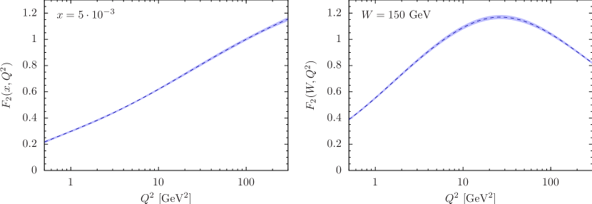
Figure 8: $Q^{2}$-dependence of the structure function $F_{2}$. On the left for fixed $x=5\cdot 10^{-3}$, on the right for fixed $W=150\,\mbox{GeV}$. $F_{2}$ shown here is obtained from the parametrisation of [32], the band indicates a $1\sigma$-uncertainty.

We shall now illustrate the convolution formula (42) for the example of the GBW model where we have, of course, the choice $\xi=x$, see (31) and (33). Furthermore we set

$$Q_{0}=\sqrt{10}\mbox{ GeV}\,,\qquad r_{0}=z_{0}/Q_{0}=0.24\mbox{ GeV}^{-1}\>\widehat{=}\>0.047\mbox{ fm}\,.$$ (46)

In Figure 9 we show for $x=10^{-3}$ the original function $S_{\mathrm{GBW}}$, suitably normalised,

$$(S\int\kappa)_{\mathrm{GBW}}(x,t):=S_{\mathrm{GBW}}(x,t)\int_{-\infty}^{\infty}\mathrm{d}\tau\,\kappa(\tau)=\left.\frac{0.15}{rr_{0}}\,\hat{\sigma}_{\mathrm{GBW}}(r,x)\right|_{r=r_{0}\exp(-t)}\,,$$ (47)

as well as the result of the convolution,

$$(S\ast\kappa)_{\mathrm{GBW}}(x,t):=\int_{-\infty}^{\infty}\mathrm{d}t^{\prime}\,\kappa(t-t^{\prime})S_{\mathrm{GBW}}(x,t^{\prime})=\left.F_{2\,\mathrm{GBW}}(x,Q^{2})\,\frac{Q_{0}}{Q}\right|_{Q=Q_{0}\exp(t)}\,.$$ (48)

The effect of the broadening due to the convolution is clearly visible in Figure 9. We also see that within a factor of 2 we have very roughly

$$(S\ast\kappa)_{\mathrm{GBW}}(x,t)\approx(S\int\kappa)_{\mathrm{GBW}}(x,t)\qquad\text{for }-3\lesssim t\lesssim 1\,.$$ (49)

This relation actually holds for a wide range in $x$, with the $t$-range varying somewhat with $x$. Translating this back to $r$ and $Q$ we find that within a factor of 2 we have

$$F_{2\,\mathrm{GBW}}(x,Q^{2})\frac{Q_{0}}{Q}\approx\left.\frac{0.15}{rr_{0}}\,\hat{\sigma}_{\mathrm{GBW}}(r,x)\right|_{r=z_{0}/Q}\qquad\text{for }\>0.2\,\mbox{GeV}\lesssim Q\lesssim 8\,\mbox{GeV}\,.$$ (50)

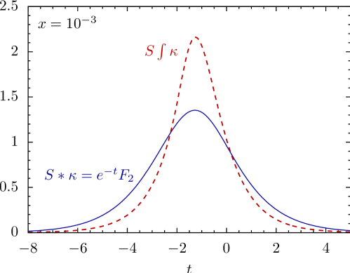
Figure 9: The functions (47) (red, dashed) and (48) (blue, solid) in the GBW model for $x=10^{-3}$.

But for large and for very small $Q^{2}$ a relation of the form (49) respectively (50) does not hold at all. In the left panel of Figure 10 we show the functions (47) and (48) of Figure 9 but multiplied by $\exp(t)$. This gives a clear indication of what happens for large $t$, that is, large $Q^{2}$ and small $r$. We see from the Figure that, for $t\gtrsim-1$, $F_{2\,\mathrm{GBW}}=e^{t}(S\ast\kappa)_{\mathrm{GBW}}$ and $e^{t}(S\int\kappa)_{\mathrm{GBW}}=0.15\,r^{-2}\hat{\sigma}_{\mathrm{GBW}}|_{r=r_{0}\exp(-t)}$ have a completely different behaviour. $F_{2\,\mathrm{GBW}}$ rises linearly with $t$, while $\hat{\sigma}_{\mathrm{GBW}}/r^{2}$ goes to a constant for $t\to\infty$, that is $r\to 0$. The latter corresponds to the assumption of colour transparency in the GBW model. Note that the derivative of a linear function of $t$ gives a constant. We shall show below that quite generally we expect indeed a derivative relation between $F_{2}(\xi,Q^{2})$ and $r^{-2}\hat{\sigma}(r,\xi)$ for large $Q^{2}$.

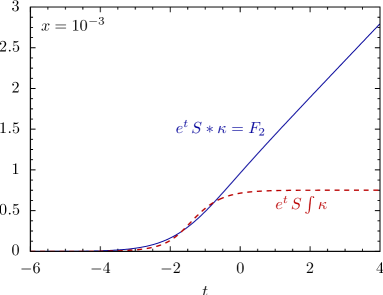
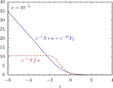
Figure 10: The two functions of Figure 9, but now multiplied by $\exp(t)$ (left panel) and $\exp(-t)$ (right panel).

In the right panel of Figure 10 we show again the functions (47) and (48) of Figure 9 but now multiplied by $\exp(-t)$. In this way we see clearly what happens for $t\to-\infty$, that is, for very small $Q^{2}$ and large $r$. For $t\to-\infty$ the function $e^{-t}S\ast\kappa=e^{-2t}F_{2}$ behaves as $(-t)$ whereas $e^{-t}S\int\kappa$ is constant, suggesting again a derivative relation between them. Indeed, we shall show below that on general grounds we expect for $t\to-\infty$ such a derivative relation between $\sigma_{T}+\sigma_{L}$ and $\hat{\sigma}$ to hold.

4.1 The large-$Q^{2}$ regime

In this subsection we give a general discussion of the convolution formula (42) for large $t$ corresponding to large $Q^{2}$ and small $r$. We rewrite (42) in the form

$$F_{2}(\xi,Q_{0}^{2}e^{2t})=\int_{-\infty}^{\infty}\mathrm{d}t^{\prime}\,\kappa(t-t^{\prime})\exp(t-t^{\prime})e^{t^{\prime}}S(\xi,t^{\prime})$$ (51)

where

$$e^{t^{\prime}}S(\xi,t^{\prime})=\left.\frac{1}{r^{2}}\hat{\sigma}(r,\xi)\right|_{r=r_{0}\exp(-t^{\prime})}\,.$$ (52)

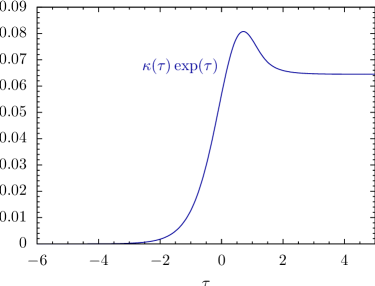
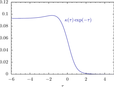
Figure 11: The functions $\kappa(\tau)\exp(\tau)$ and $\kappa(\tau)\exp(-\tau)$.

The function $\kappa(\tau)\exp(\tau)$ is shown in the left panel of Figure 11. Very roughly it resembles a step function. Suppose now that $\hat{\sigma}(r,\xi)/r^{2}$ is slowly varying for $r\to 0$ corresponding to $\exp(t^{\prime})S(\xi,t^{\prime})$ being slowly varying for $t^{\prime}\to\infty$. In (51) this function is folded with $\kappa(t-t^{\prime})\exp(t-t^{\prime})$ which resembles a step function. The folding produces, therefore, in essence the primitive of $\exp(t)S(\xi,t)$. That is, we expect for large $t$ the following relation to hold

$$c_{\infty}e^{t}S(\xi,t)\approx\frac{\partial}{\partial t}\,F_{2}(\xi,Q_{0}^{2}e^{2t})\qquad(t\gg 1)\,,$$ (53)

respectively

$$c_{\infty}\frac{1}{r^{2}}\,\hat{\sigma}(r,\xi)\approx\left.2\,Q^{2}\frac{\partial}{\partial Q^{2}}\,F_{2}(\xi,Q^{2})\right|_{Q^{2}=(z_{0}/r)^{2}}\qquad(Q^{2}\gg 74\,\mbox{GeV})\,,$$ (54)

with

$$c_{\infty}:=2\pi(\kappa(\tau)\left.\exp(\tau))\right|_{\tau\to\infty}=\frac{2}{\pi^{3}}=0.065\,.$$ (55)

This is illustrated for the GBW model in the left panel of Figure 12 for the choice $x=10^{-3}$. Here the relation (53) respectively (54) is indeed well confirmed for $t>0$ corresponding to $Q^{2}>10~{}\mbox{GeV}^{2}$.

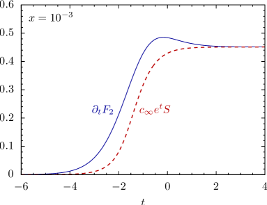
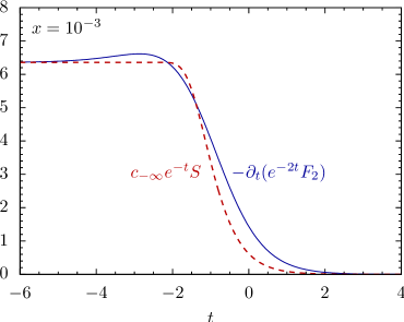
Figure 12: Numerical test of the derivative relations (53) respectively (54) (left panel) and (59) respectively (60) (right panel) for the GBW model for $x=10^{-3}$.

From (54) we see that the dipole formula will work well phenomenologically at high $Q^{2}$ if we choose an energy variable $\xi$ such that $F_{2}(\xi,Q^{2})$ increases with $Q^{2}$ at fixed $\xi$ since then the cross section $\hat{\sigma}$ can be positive. This is the case for the choice $\xi=x$ for small $x$ but, of course, many other choices of $\xi$ would also have this property. On the other hand, $F_{2}(W,Q^{2})$ decreases for fixed $W$ at large enough $Q^{2}$, see figure 8. Therefore, it is clear that dipole models with the choice $\hat{\sigma}(r,W)$ will only be able to describe the structure function $F_{2}(W,Q^{2})$ over a more limited range of $Q^{2}$ values. But this limitation at high $Q^{2}$ is as it should be and is physically reasonable as explained in [16, 17, 18]. Therefore, this should by no means be used as argument against the choice of the energy variable $W$.

4.2 The small-$Q^{2}$ regime

To study the dipole formula in the small-$Q^{2}$ regime, that is for $t\to-\infty$, we rewrite (42) in the following form

$$F_{2}(\xi,Q_{0}^{2}e^{2t})e^{-2t}=\int_{-\infty}^{\infty}\mathrm{d}t^{\prime}\,\kappa(t-t^{\prime})\exp[-(t-t^{\prime})]\exp(-t^{\prime})S(\xi,t^{\prime})\,.$$ (56)

The function $\kappa(\tau)\exp(-\tau)$ resembles very roughly a downward step function, see the right panel of Figure 11. Furthermore we have

$$\exp(-t)S(\xi,t)=\left.\frac{1}{r_{0}^{2}}\,\hat{\sigma}(r,\xi)\right|_{r=r_{0}\exp(-t)}\,,$$ (57)

and we study here the limit $t\to-\infty$, that is, the limit of large $r$. Let us assume now that $\hat{\sigma}(r,\xi)$ is a smooth, only slowly varying, function of $r$ for $r\to\infty$. This is, for instance, the case for dipole models where the dipole-proton cross section saturates for $r\to\infty$,

$$\hat{\sigma}(r,\xi)\rightarrow\sigma_{0}\qquad\text{for }\>r\to\infty\,.$$ (58)

Now we can apply the same type of argument as we used for the large-$Q^{2}$ regime. In (56) the slowly varying function $\exp(-t^{\prime})S(\xi,t^{\prime})$ is, for $t\to-\infty$, folded with a function resembling a downward step function. Thus, we get an approximate derivative relation

$$c_{-\infty}\exp(-t)S(\xi,t)\approx-\frac{\partial}{\partial t}\left[F_{2}(\xi,Q_{0}^{2}e^{2t})e^{-2t})\right]\,,$$ (59)

or, put differently,

$$c_{-\infty}\frac{1}{r_{0}^{2}}\hat{\sigma}(r,\xi)\approx\frac{Q_{0}^{2}}{4\pi^{2}\alpha_{\mathrm{em}}}\left.(-2)\,Q^{2}\frac{\partial}{\partial Q^{2}}\,[\sigma_{T}(\xi,Q^{2})+\sigma_{L}(\xi,Q^{2})]\right|_{Q^{2}=(z_{0}/r)^{2}}\,,$$ (60)

where

$$c_{-\infty}:=2\pi(\kappa(\tau)\left.\exp(-\tau))\right|_{\tau\to-\infty}=\frac{z_{0}^{2}}{2\pi^{3}}=0.093\,.$$ (61)

In the right panel of Figure 12 we show for the GBW model the functions of the l.h.s. and r.h.s. of (59). We see that there is indeed approximate equality of the two functions for $t<-2$. Translated into cross section implies (60) to hold for $Q^{2}<0.2\,\mbox{GeV}^{2}$. These are extremely small $Q^{2}$, and the actual relation is therefore more of academic than of phenomenological interest. Nevertheless, we find it useful to discuss its meaning. As we will show now, (60) gives interesting insight concerning the approximations underlying the dipole picture.

The result (60) is somewhat surprising. It means the following. The dipole model with energy variable $\xi$ can only work down to very small $Q^{2}$ with non-negative cross section $\hat{\sigma}(r,\xi)$ if $\sigma_{T}(\xi,Q^{2})+\sigma_{L}(\xi,Q^{2})$ increases with decreasing $Q^{2}$ for small $Q^{2}$. A saturating dipole cross section

$$\hat{\sigma}(r,\xi)\rightarrow\sigma_{0}\neq 0\qquad\text{for }\>r\to\infty$$ (62)

implies a logarithmic increase of $\sigma_{T}+\sigma_{L}$:

$$\sigma_{T}(\xi,Q^{2})+\sigma_{L}(\xi,Q^{2})\propto\ln(Q_{0}^{2}/Q^{2})\qquad\text{for }\>Q^{2}\to 0\,.$$ (63)

Clearly, the behaviour (63) is unacceptable physically. For the case $\xi=W$ we know that gauge invariance requires the behaviour

$$\sigma_{T}(W,Q^{2})+\sigma_{L}(W,Q^{2})\rightarrow\text{const.}\qquad\text{for }\>Q^{2}\to 0\,.$$ (64)

Indeed, a realistic behaviour for $Q^{2}\to 0$ is

$$\sigma_{T}(W,Q^{2})+\sigma_{L}(W,Q^{2})=\sigma_{\gamma p}(W)\left(1-\frac{Q^{2}}{m^{2}_{\rm eff}}+\mathcal{O}(Q^{4})\right)\,,$$ (65)

where $\sigma_{\gamma p}(W)$ is the real-photon-proton cross section and $m^{2}_{\rm eff}>0$ is a constant of dimension mass squared. Inserting (65) in (60) leads to

$$\hat{\sigma}(r,W)\approx\frac{1}{c_{-\infty}}\,\frac{z_{0}^{4}\sigma_{\gamma p}(W)}{2\pi^{2}\alpha_{\rm em}}\frac{1}{r^{2}m^{2}_{\rm eff}}\left(1+\mathcal{O}\left(\frac{r_{0}^{2}}{r^{2}}\right)\right)$$ (66)

for $r\to\infty$.

Thus, we have two options. We can either assume that the naive dipole picture with the standard perturbative photon wave functions holds down to very small $Q^{2}$ values. Then, the above arguments force us to give up the saturation hypothesis (62) for the dipole-proton cross section $\hat{\sigma}(r,W)$ which should then instead vanish as $1/r^{2}$ for $r\to\infty$, see (66). We think, however, that the more likely resolution of the above puzzle is that the naive dipole picture must be modified for small $Q^{2}$. But we know already from the discussions in [16, 17, 18] that the naive dipole picture is expected to break down for small $Q^{2}$, where the estimate was $Q^{2}\lesssim 2~{}\mbox{GeV}^{2}$. Thus, the discussion above gives further evidence for this breakdown.

In [16] a general analysis of the modifications and additions to the photon wave functions and the dipole cross section to be expected for small $Q^{2}$ was given. We believe that these corrections are relevant in the context of the discussion above. On a more phenomenological level, one can also cure the problem by introducing modifications of the photon wave functions, as done for instance in [23], and get then a reconciliation of (62) and (64). The implementation of vector meson dominance at small $Q^{2}$ has similar effects with regard to the problem pointed out here.

5 Conclusions

The dipole model is widely used in the analysis of deep inelastic scattering data, but also in other processes. Often one attempts to extract subtle effects from the data with the help of the dipole picture, for example the presence or absence of saturation effects. Many of these studies use Bjorken-$x$ as the energy variable in the dipole cross section $\hat{\sigma}$. However, general considerations based on quantum field theory lead to the conclusion that the correct energy variable in $\hat{\sigma}$ is $W$. In particular, the dipole cross section has to be independent of the photon virtuality $Q^{2}$. This issue of the energy variable in $\hat{\sigma}$ has not been taken very seriously so far, since the integral over dipole sizes is thought to be dominated by dipoles of a typical size $r\sim 1/Q$. Assuming the strong dominance of a typical dipole size one can freely change from one energy variable to another, in particular from $W$ to $x$ and vice versa. We have shown here that this simple picture is misleading. In particular, we have shown that the corresponding change of energy variable has a large effect on the resulting structure function for any given model of the dipole cross section. Numerically, the resulting effect is sizeable and can easily exceed the spread among different models for $\hat{\sigma}$ suggested in the literature. For a reliable study of subtle effects in the data the correct choice of energy variable hence appears much more important than has been previously assumed.

Apart from the numerical consequences of choosing energy variables other than $W$ in the dipole cross section there is also an important conceptual reason for choosing $W$. With the variables used in (8) that formula is an actual factorisation: the variables of the l.h.s., $Q^{2}$ and $W$, are separated and occur in two different factors in the integrand on the r.h.s. If the second factor in the integrand on the r.h.s. would still contain $x$ and hence $Q^{2}$, the dipole formula would not constitute a factorisation. This would spoil the familiar (and correct) picture of photon-proton scattering as a two-step process: the photon fluctuating into a quantum-mechanical superposition of dipoles of all possible sizes and the subsequent dipole-proton scattering. The photon virtuality $Q^{2}$ determines the probability distribution of dipole sizes, but a dipole of given size does not inherit any information on $Q^{2}$. Its subsequent scattering on the proton hence cannot depend on $Q^{2}$. If, as is usually done in the dipole picture for DIS, the second step is interpreted as the cross section of asymptotic dipole states on the proton, the use of an energy variable involving $Q^{2}$ in the dipole cross section would violate the rules of quantum field theory.

In the second part of the paper we have shown that the dipole formula can be written such that the structure function $F_{2}$ is represented by a convolution of the (suitably rescaled) dipole cross section with a known function originating from the photon wave functions. In principle, this convolution could even be invertible, albeit with some caveats. While a precise determination of the dipole cross section from $F_{2}$ based on inversion of the convolution appears very difficult we have found that the asymptotic behaviour of the dipole cross section $\hat{\sigma}(r,\xi)$ for small and large $r$ can be extracted from $F_{2}$ (even for any given choice of energy variable $\xi$). In particular, we have found derivative relations between $F_{2}$ and the dipole cross section for both large and very small $Q^{2}$. We expect that these findings can be used to construct improved models for the dipole cross section.

Further, we have been able to explain why in general dipole models using the energy variable $x$ are better suited for fitting $F_{2}$ in a wide range of kinematic parameters than models using the correct variable $W$. Based on the representation of the dipole formula as a convolution this can be directly traced back to the sign of the scaling violations that occur for increasing $Q^{2}$ at fixed small $x$. In our opinion that does not disfavour the choice of $W$ as energy variable in the dipole cross section. On the contrary, the dipole model clearly contains approximations implying already a priori a limited kinematic range for its applicability. As shown in [16, 17, 18] the choice of $W$ as energy variable leads to such limits which are physically reasonable.

Appendix A Integrated photon densities

In this appendix we derive the asymptotic behaviour of the (over longitudinal momentum fraction $\alpha$) integrated photon densities $w_{T,L}^{(q)}(r,Q^{2})$, defined in (9) and (10), at small and large distances $r$. In the main text these limits are needed only for massless quarks. For completeness we give them for massive quarks as well.

At small distances, $rQ\ll 1$ and $rm_{q}\ll 1$, we find from (11) and (12)

$$w_{T}^{(q)}(r,Q^{2}) \,\xrightarrow{r\rightarrow 0}\,\frac{N_{c}\alpha_{\mathrm{em}}Q_{q}^{2}}{2\pi^{2}}\,Q^{2}\frac{2}{3}\,\frac{1}{(Qr)^{2}}\,,$$ (67)

$$w_{L}^{(q)}(r,Q^{2}) \,\xrightarrow{r\rightarrow 0}\,\frac{2N_{c}\alpha_{\mathrm{em}}Q_{q}^{2}}{\pi^{2}}\,Q^{2}\frac{1}{30}\,\ln^{2}(Qr)\,.$$ (68)

Note that these leading terms are independent of $m_{q}$.

For the limits at large distances we consider massless quarks and massive quarks separately. For massless quarks, $m_{q}=0$, we find without any approximation

$$w_{T}^{(q)}(r,Q^{2}) =\frac{N_{c}\alpha_{\mathrm{em}}Q_{q}^{2}}{2\pi^{2}}\,Q^{2}\frac{2\pi}{(Qr)^{6}}\Bigg{[}2\,G^{3,1}_{2,4}\left(\frac{1}{4}(Qr)^{2}\left|{\begin{array}[]{l}2,7/2\\ 2,3,4,3/2\end{array}}\right.\right)$$ (71)

$$\qquad\qquad\qquad\qquad\qquad-G^{3,1}_{2,4}\left(\frac{1}{4}(Qr)^{2}\left|{\begin{array}[]{l}1,7/2\\ 2,3,4,1/2\end{array}}\right.\right)\Bigg{]},$$ (74)

$$w_{L}^{(q)}(r,Q^{2}) =\frac{2N_{c}\alpha_{\mathrm{em}}Q_{q}^{2}}{\pi^{2}}\,Q^{2}\frac{\pi}{(Qr)^{6}}\,G^{3,1}_{2,4}\left(\frac{1}{4}(Qr)^{2}\left|{\begin{array}[]{l}1,7/2\\ 3,3,3,1/2\end{array}}\right.\right)$$ (77)

with Meijer’s $G$-function. From this we get at large distances, $rQ\gg 1$:

$$w_{T}^{(q)}(r,Q^{2}) \,\xrightarrow{r\rightarrow\infty}\,\frac{N_{c}\alpha_{\mathrm{em}}Q_{q}^{2}}{2\pi^{2}}\,Q^{2}\frac{8}{3}\,\frac{1}{(Qr)^{4}}\,,$$ (78)

$$w_{L}^{(q)}(r,Q^{2}) \,\xrightarrow{r\rightarrow\infty}\,\frac{2N_{c}\alpha_{\mathrm{em}}Q_{q}^{2}}{\pi^{2}}\,Q^{2}\frac{64}{15}\,\frac{1}{(Qr)^{6}}\,.$$ (79)

For massive quarks, $m_{q}>0$, and large distances, $rQ\gg 1$ and $r\,m_{q}\gg 1$, our calculation for $w_{T}^{(q)}$ and conjecture for $w_{L}^{(q)}$ give

$$w_{T}^{(q)}(r,Q^{2}) \,\xrightarrow{r\rightarrow\infty}\,\frac{N_{c}\alpha_{\mathrm{em}}Q_{q}^{2}}{2\pi^{2}}\,Q^{2}\frac{\pi m_{q}}{Q}\,\frac{\exp(-2m_{q}r)}{Qr}\,,$$ (80)

$$w_{L}^{(q)}(r,Q^{2}) \,\xrightarrow{r\rightarrow\infty}\,\frac{2N_{c}\alpha_{\mathrm{em}}Q_{q}^{2}}{\pi^{2}}\,Q^{2}\frac{\pi Q}{2m_{q}}\,\eta(m_{q}/Q)\,\frac{\exp(-2m_{q}r)}{(Qr)^{3}}$$ (81)

with some $r$-independent function $\eta(m_{q}/Q)$ for which we find in the case $m_{q}<Q$ the numerical value $\eta(m_{q}/Q)\approx 0.25$ independent of $m_{q}/Q$. The formula (81) is based on the assumption that for large $r$ the factor multiplying $\exp(-2m_{q}r)$ can be expanded in a series in $1/r$, and the leading exponent has been determined numerically.

Figure 13 shows the photon densities as functions of the dipole size $r$ together with the asymptotic expressions given above.

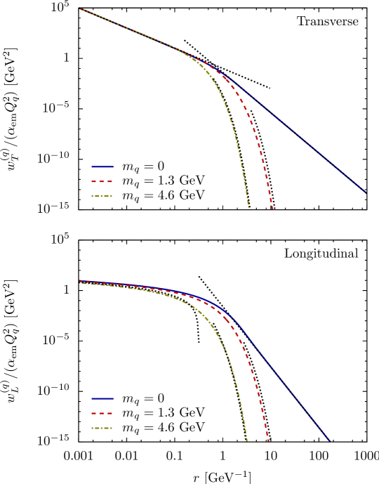
Figure 13: Integrated photon densities $w_{T}^{(q)}(r,Q^{2})$ (upper plot) and $w_{L}^{(q)}(r,Q^{2})$ (lower plot), both normalised to $\alpha_{\text{em}}Q_{q}^{2}$, as a function of the dipole size $r$. In addition, the leading terms for small and large $r$ are shown as dotted curves. The photon virtuality is fixed to $Q^{2}=10$ GeV².

Appendix B A simplified version of the Donnachie-Dosch model

In section 3 we have used a simplified version of the Donnachie-Dosch model of [29]. In this appendix we briefly describe how the simplified model used in the present paper is obtained from the original model.

We start from eq. (3) of [29] which is the cross section for the scattering of two dipoles of sizes $R_{1}$ and $R_{2}$,

$$\sigma_{\text{dip}}(R_{1},R_{2})=0.67\,\frac{1}{4\pi}(\langle g^{2}FF\rangle a^{4})^{2}\,R_{1}\left(1-e^{-\frac{R_{1}}{3.1\,a}}\right)R_{2}\left(1-e^{-\frac{R_{2}}{3.1\,a}}\right)\,,$$ (82)

with the parameter $a=0.346\,\mbox{fm}$ and the gluon condensate $\langle g^{2}FF\rangle$ taken from lattice results, $\langle g^{2}FF\rangle a^{4}=23.77$. The cross section for photons or hadrons as external particles is obtained by folding the dipole-dipole cross section with the respective wave functions. This is given in [29] for the process $ab\to cb$. For our case of the elastic amplitude $\gamma^{*}p\to\gamma^{*}p$ these wave functions are those of the photon and of the proton. In [29] the latter is

$$\psi_{p}(R)=\frac{1}{\sqrt{2\pi}R_{p}}\,\exp\left(-\frac{R^{2}}{4R_{p}^{2}}\right)$$ (83)

with $R_{p}=0.75\,\mbox{fm}$. Combining formulae (2) and (5) of [29] and relabelling $R_{1}$ as our $r$ this leads to our formulae (8)-(10) with

$$\hat{\sigma}(r)=\int\mathrm{d}^{2}R_{2}\,\left|\psi_{p}(R_{2})\right|^{2}\sigma_{\text{dip}}(r,R_{2})\,.$$ (84)

In addition, an energy dependence of the dipole cross section is introduced by hand in [29]. It represents the exchanges of a soft and of a hard pomeron. The soft pomeron contributes only if both dipoles are larger than a certain $R_{c}$, chosen to be $R_{c}=0.22\,\mbox{fm}$. The hard pomeron contributes only if at least one of the two dipoles is smaller than $R_{c}$. This leads to four different integration regions in the integrals over the two dipole sizes, according to whether $r$ and/or $R_{2}$ are smaller or larger than $R_{c}$. In our simplified model we assume instead that the soft pomeron is the only contribution if $r$ (the size of the $q\bar{q}$ pair originating from the photon) is larger than $R_{c}$, and the hard pomeron is the only contribution if $r<R_{c}$, independently of the size of $R_{2}$ relative to $R_{c}$.

Taking into account only these two contributions with their assumed energy behaviour we have, similar to eq. (14) of [29],

$$\hat{\sigma}(r,W)=\theta(r-R_{c})\,\hat{\sigma}_{s}(r)\left(\frac{W}{W_{0}}\right)^{2\epsilon_{s}}+\theta(R_{c}-r)\,\hat{\sigma}_{h}(r)\left(\frac{W}{W_{0}}\right)^{2\epsilon_{h}}$$ (85)

with the parameters given in (3.2). The theta-functions indicate where the two contributions are relevant. Here $\hat{\sigma}_{s}$ is given by the $R_{2}$-dependent factors of eq. (16) of [29], that is by (84) above. The contribution $\hat{\sigma}_{h}$, on the other hand, is obtained from eq. (17) of [29] by dropping the integral over $R_{1}$ and the photon wave functions. As explained above we take into account only the contribution where $r<R_{c}$, but integrate over all dipole sizes in the proton. In eq. (17) of [29] this corresponds to only the second of the three integrals there, with the lower limit of the $R_{2}$-integration set to zero. Accordingly,

$$\hat{\sigma}_{h}(r)=\int_{0}^{\infty}2\pi R_{2}\,\mathrm{d}R_{2}\,\left|\psi_{p}(R_{2})\right|^{2}\sigma_{\text{dip}}(r,R_{2})\left(\frac{r}{R_{c}}\right)^{2\epsilon_{h}}\,.$$ (86)

The integral over $R_{2}$ occurring in (84) and (86) can be performed numerically. Concentrating on the $R_{2}$-dependent factors only we have

$$\int\mathrm{d}^{2}R_{2}\,\left|\psi_{p}(R_{2})\right|^{2}R_{2}\left(1-e^{-\frac{R_{2}}{3.1\,a}}\right)=0.60\,\mbox{fm}\,.$$ (87)

Collecting all factors, we finally arrive at the simplified model (25) with the parameters (3.2).

Finally, the original model of [29] introduces a rescaling of the dipole cross section by the running coupling $\alpha_{s}(Q^{2})$, see eq. (13) there. That rescaling is relevant in particular at large $Q^{2}$. We leave out this factor in order to avoid a $Q^{2}$-dependence of the dipole cross section.

References

- [1] N. N. Nikolaev and B. G. Zakharov, Colour transparency and scaling properties of nuclear shadowing in deep inelastic scattering, Z. Phys. C 49 (1991) 607
- [2] N. N. Nikolaev and B. G. Zakharov, Pomeron structure function and diffraction dissociation of virtual photons in perturbative QCD, Z. Phys. C 53 (1992) 331
- [3] A. H. Mueller, Soft gluons in the infinite momentum wave function and the BFKL pomeron, Nucl. Phys. B 415 (1994) 373
- [4] J. Breitweg et al. [ZEUS Collaboration], Measurement of the proton structure function at very low at HERA, Phys. Lett. B 487 (2000) 53 [arXiv:hep-ex/0005018]
- [5] C. Adloff et al. [H1 Collaboration], Deep-inelastic inclusive scattering at low x and a determination of , Eur. Phys. J. C 21 (2001) 33 [arXiv:hep-ex/0012053]
- [6] S. Chekanov et al. [ZEUS Collaboration], Measurement of the neutral current cross section and structure function for deep inelastic scattering at HERA, Eur. Phys. J. C 21 (2001) 443 [arXiv:hep-ex/0105090]
- [7] C. Adloff et al. [H1 Collaboration], Measurement and QCD analysis of neutral and charged current cross sections at HERA, Eur. Phys. J. C 30 (2003) 1 [arXiv:hep-ex/0304003]
- [8] S. Chekanov et al. [ZEUS Collaboration], High- neutral current cross sections in deep inelastic scattering at 318 GeV, Phys. Rev. D 70 (2004) 052001 [arXiv:hep-ex/0401003]
- [9] F. D. Aaron et al. [H1 Collaboration and ZEUS Collaboration], Combined measurement and QCD analysis of the inclusive ep scattering cross sections at HERA, JHEP 1001 (2010) 109 [arXiv:0911.0884 [hep-ex]].
- [10] C. Aidala et al., The EIC Working Group, A high luminosity, high energy electron-ion-collider - A white paper prepared for the NSAC LRP 2007, http://web.mit.edu/eicc/DOCUMENTS/EIC_LRP-20070424.pdf
- [11] T. H. Bauer, R. D. Spital, D. R. Yennie and F. M. Pipkin, The hadronic properties of the photon in high-energy interactions, Rev. Mod. Phys. 50 (1978) 261 [Erratum ibid. 51 (1979) 407]
- [12] D. Schildknecht, Vector meson dominance, Acta Phys. Polon. B 37 (2006) 595 [arXiv:hep-ph/0511090].
- [13] S. Donnachie, H. G. Dosch, O. Nachtmann, and P. Landshoff, Pomeron physics and QCD, Cambridge University Press, 2002
- [14] F. Close, S. Donnachie and G. Shaw (editors) Electromagnetic interactions and hadronic structure, Cambridge University Press, 2007
- [15] C. Ewerz and O. Nachtmann, Towards a nonperturbative foundation of the dipole picture: I. Functional methods, Annals Phys. 322 (2007) 1635 [arXiv:hep-ph/0404254]
- [16] C. Ewerz and O. Nachtmann, Towards a nonperturbative foundation of the dipole picture: II. High energy limit, Annals Phys. 322 (2007) 1670 [arXiv:hep-ph/0604087]
- [17] C. Ewerz and O. Nachtmann, Bounds on ratios of DIS structure functions from the color dipole picture, Phys. Lett. B 648 (2007) 279 [arXiv:hep-ph/0611076]
- [18] C. Ewerz, A. von Manteuffel, and O. Nachtmann, On the range of validity of the dipole picture, Phys. Rev. D 77 (2008) 074022 [arXiv:0708.3455 [hep-ph]]
- [19] K. J. Golec-Biernat and M. Wüsthoff, Saturation effects in deep inelastic scattering at low and its implications on diffraction, Phys. Rev. D 59 (1998) 014017 [arXiv:hep-ph/9807513]
- [20] J. Bartels, K. J. Golec-Biernat and H. Kowalski, A modification of the saturation model: DGLAP evolution, Phys. Rev. D 66 (2002) 014001 [arXiv:hep-ph/0203258].
- [21] E. Iancu, K. Itakura and S. Munier, Saturation and BFKL dynamics in the HERA data at small x, Phys. Lett. B 590 (2004) 199 [arXiv:hep-ph/0310338].
- [22] J. L. Albacete, N. Armesto, J. G. Milhano and C. A. Salgado, Non-linear QCD meets data: A global analysis of lepton-proton scattering with running coupling BK evolution, Phys. Rev. D 80 (2009) 034031 [arXiv:0902.1112 [hep-ph]].
- [23] H. G. Dosch, T. Gousset and H. J. Pirner, Nonperturbative p interaction in the diffractive regime, Phys. Rev. D 57 (1998) 1666 [arXiv:hep-ph/9707264].
- [24] J. R. Forshaw, G. Kerley and G. Shaw, Extracting the dipole cross-section from photo- and electro-production total cross-section data, Phys. Rev. D 60 (1999) 074012 [arXiv:hep-ph/9903341].
- [25] H. Kowalski and D. Teaney, An impact parameter dipole saturation model, Phys. Rev. D 68 (2003) 114005 [arXiv:hep-ph/0304189].
- [26] G. Watt and H. Kowalski, Impact parameter dependent colour glass condensate dipole model, Phys. Rev. D 78 (2008) 014016 [arXiv:0712.2670 [hep-ph]].
- [27] L. Motyka, K. Golec-Biernat and G. Watt, Dipole models and parton saturation in ep scattering, arXiv:0809.4191 [hep-ph].
- [28] G. Cvetic, D. Schildknecht, B. Surrow and M. Tentyukov, The generalized vector dominance/ colour-dipole picture of deep-inelastic scattering at low x, Eur. Phys. J. C 20 (2001) 77 [arXiv:hep-ph/0102229].
- [29] A. Donnachie and H. G. Dosch, A comprehensive approach to structure functions, Phys. Rev. D 65 (2002) 014019 [arXiv:hep-ph/0106169v1].
- [30] O. Nachtmann, Elementary particle physics: Concepts and phenomena, Springer Verlag, Berlin, Heidelberg, 1990
- [31] L. N. Hand, Experimental investigation of pion electroproduction, Phys. Rev. 129 (1963) 1834.
- [32] L. Del Debbio, S. Forte, J. I. Latorre, A. Piccione and J. Rojo [NNPDF Collaboration], Unbiased determination of the proton structure function with faithful uncertainty estimation, JHEP 0503 (2005) 080 [arXiv:hep-ph/0501067].