On the Capacity of the Heat Channel, Waterfilling in the Time-Frequency Plane, and a C-NODE Relationship

Abstract

The heat channel is defined by a linear time-varying (LTV) filter with additive white Gaussian noise (AWGN) at the filter output. The continuous-time LTV filter is related to the heat kernel of the quantum mechanical harmonic oscillator, so the name of the channel. The channel’s capacity is given in closed form by means of the Lambert W function. Also a waterfilling theorem in the time-frequency plane for the capacity is derived. It relies on a specific Szegő theorem for which an essentially self-contained proof is provided. Similarly, the rate distortion function for a related nonstationary source is given in closed form and a (reverse) waterfilling theorem in the time-frequency plane is derived. Finally, a second closed-form expression for the capacity of the heat channel based on the detected perturbed filter output signals is presented. In this context, a precise differential connection between channel capacity and the normalized optimal detection error (NODE) is revealed. This C-NODE relationship is compared with the well-known I-MMSE relationship connecting mutual information with the minimum mean-square error (MMSE) of estimation theory.

1 Introduction

The conduction of heat in solid bodies was mathematically described and solved by Joseph Fourier in his fundamental 1822 treatise Théorie analytique de la chaleur [2]. In one dimension, e.g., in case of a heat-conducting insulated wire, his description results in the partial differential equation (known as heat equation)

$$\frac{\partial u}{\partial t}=k\frac{\partial^{2}u}{\partial x^{2}},$$

in which $u=u(x,t)$ is temperature at time $t\geq 0$ at any point $x$ and $k$ is a positive constant depending on the material. Given the initial temperature distribution $f(x)$ for a wire of infinite length, Fourier’s solution to the heat equation is

$$u(x,t)=\frac{1}{\sqrt{4\pi kt}}\int_{-\infty}^{\infty}e^{-\frac{(x-y)^{2}}{4kt}}f(y)\,\mathrm{d}y.$$ (1)

Since, in general, for any time $t>0$ the inversion of the integral transform appearing in (1) is unfeasible in practice [3], we observe an unavoidable loss of “information” (in a preliminary, informal sense). In Fig. 1, several temperature distributions $u(x,t)$ are depicted showing how the initial one is gradually smeared out by the propagation of heat.

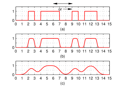
Figure 1: Spreading of heat/signal spread because of dispersion in an optical fiber (attenuation not regarded). (a) Initial temperature distribution/fiber input signal. (b) Temperature, shortly after/output signal, short fiber. (c) Temperature, later time/output signal, longer fiber. Arrows indicate direction of spatial propagation of heat ($\leftrightarrow$) or optical intensity ($\rightarrow$).

A similar situation, in principle known since the earliest days of cable communication [4], arises in fiber optics. In a transmission through a (single-mode) optical fiber, signals experience besides attenuation a spread over time due to (chromatic) dispersion (see, e.g., [5], [6]). A frequently used model for dispersion in an optical fiber [5] is a linear time-invariant (LTI) filter with impulse response (cf. Fig. 2)

$$h_{1}(t)=\frac{1}{\sqrt{2\pi}(1/\beta)}e^{-\frac{1}{2}\frac{t^{2}}{(1/\beta)^{2}}},$$ (2)

i.e., a Gaussian filter with the standard deviation $1/\beta$, $\beta\in(0,\infty)$ characterizing dispersion (the parametrization is chosen to fit later notation). The fiber input/output relation is now given by the convolution integral

$$u(t)=a\int_{-\infty}^{\infty}h_{1}(t-t^{\prime})f(t^{\prime})\,\mathrm{d}t^{\prime},$$ (3)

where $f\in L^{2}(\mathbb{R})$ is the finite-energy input signal and $u(t)$ the output, the constant factor $a\in(0,1]$ representing attenuation. Except for the factor $a$ and change of physical dimension from position (variable $x$) to time (variable $t$), we now observe perfect analogy between Eqs. (1) and (3). As a consequence, in Fig. 1 also the degradation of an optical signal—initially a sequence of bits (here, binary symbols) obtained by intensity modulation and on-off keying—by dispersion in an optical fiber is displayed. Obviously, dispersion limits the information throughput of an optical fiber because of intersymbol interference (ISI). A maximum attainable bit rate can be estimated by considering as fiber input a sequence of unit impulses separated by time intervals of duration $\Delta t$, the output then being a sequence of Gaussian pulses of standard deviation $\tau=1/\beta$. In order to cope with ISI, a popular criterion is $\tau\leq\Delta t/4$ [5] resulting in our case for the bit rate $R_{b}=1/{\Delta t}$ (in binary symbols per second) in the estimate

$$R_{b}\leq\frac{\beta}{4}.$$ (4)

If the fiber output signal is corrupted by noise, this rule of thumb becomes questionable. In case of AWGN, typically caused by an optical amplifier [5], [7], we arrive at a continuous-time (or waveform) channel following the model in Gallager’s book [8]; see Fig. 2(a). Here, of course, we supposed that, e.g., the power spectral density (PSD) of the AWGN is independent of the input (see [9] for an opposite situation), and the input power is not so high that arising nonlinearities [5] would destroy the linear model (3); we refer to [6] for a variety of possible other perturbations that limit the capacity of optical fiber communication systems.

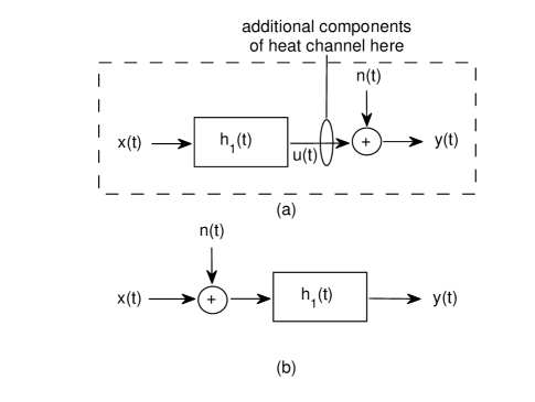
Figure 2: Continuous-time channels. (a) Gallager model [8, Fig. 8.4.1] (in dashed box) with LTI filter with impulse response $h_{1}(t)$. (b) Bandlimited Gaussian Channel; here the LTI filter is an ideal low-pass filter. Input signal $x(t)$ always power-limited; noise signal $n(t)$ realization of white Gaussian noise.

In this paper we investigate the LTV filter (or operator) $\boldsymbol{P}_{\delta}^{(\gamma)}:L^{2}(\mathbb{R})\rightarrow L^{2}(\mathbb{R})$ given by

$$(\boldsymbol{P}_{\delta}^{(\gamma)}f)(t) =e^{-\frac{t^{2}}{2\alpha^{2}}}$$ (5)

$$\cdot\frac{\beta}{\sqrt{2\pi\cosh\delta}}\int_{-\infty}^{\infty}\exp\left[-\frac{\beta^{2}}{2}\left(\frac{t}{\cosh\delta}-t^{\prime}\right)^{2}\right]f(t^{\prime})\,\mathrm{d}t^{\prime},$$

where $t$ is time and $\alpha,\,\beta$ are any positive numbers satisfying $\alpha\beta>1$ and the positive parameters $\gamma,\,\delta$ are defined by $\gamma^{2}=\alpha/\beta$, $\coth\delta=\alpha\beta$. This operator, in its original form introduced as time-frequency localization operator in signal analysis [13], was used in the present form as prefilter in a sampling theorem [16]. The Fourier transform of the filter output signal $g=\boldsymbol{P}_{\delta}^{(\gamma)}f$ is

$$\hat{g}(\omega) =e^{-\frac{\omega^{2}}{2\beta^{2}}}$$ (6)

$$\cdot\frac{\alpha}{\sqrt{2\pi\cosh\delta}}\int_{-\infty}^{\infty}\exp\left[-\frac{\alpha^{2}}{2}\left(\frac{\omega}{\cosh\delta}-\omega^{\prime}\right)^{2}\right]\hat{f}(\omega^{\prime})\,\mathrm{d}\omega^{\prime},$$

where $\omega$ is angular frequency and for the Fourier transform the convention $\hat{f}(\omega)=(2\pi)^{-1/2}\int_{-\infty}^{\infty}e^{-it\omega}f(t)\,\mathrm{d}t$ has been used [12]. The condition $\alpha\beta>1$ is now seen as imposed by the uncertainty principle of communications [17]. Interestingly enough, the kernel of operator $\boldsymbol{P}_{\delta}^{(\gamma)}$ coincides with the heat kernel [18] of the quantum mechanical harmonic oscillator. Because of the Gaussian prefactor on the right-hand side (RHS) of Eq. (6), the Fourier transform $\hat{g}(\omega)$ of the filter output signal decays exponentially outside of the interval $[-\pi\beta,\pi\beta]$ [provided that the energy of the input signal $f(t)$ is not too high]. Thus, $g(t)$ may be considered an approximately bandlimited signal of approximate bandwidth $W=\beta/2$ in positive frequencies measured in hertz.

If $u(t)$ is the output signal of the LTI filter (3) (where $a=1$) with impulse response (2) upon input signal $f(t)$, then the output signal $g(t)$ of the LTV filter (5) may be written as

$$g(t)=e^{-\frac{t^{2}}{2\alpha^{2}}}\cdot(\cosh\delta)^{-\frac{1}{2}}u(t/\cosh\delta).$$ (7)

Thus, $g(t)$ is just the dilated LTI filter output signal $u(t)$ multiplied with a Gaussian time window. In Fig. 2(a), those two operations are quoted as additional components of the heat channel, the latter meaning the continuous-time LTV channel formed by the LTV filter (5) and subsequent AWGN. As a consequence, the heat channel can be used to lower bound the capacity of an optical fiber in the presence of dispersion and AWGN. It will also allow us to design short-time pulses attaining that bound.

2 The Heat Channel

Definition 1.

The heat channel is the continuous-time LTV channel

$$\tilde{g}(t)=(\boldsymbol{P}_{\delta}^{(\gamma)}f)(t)+n(t),\,-\infty<t<\infty,$$ (8)

where $\boldsymbol{P}_{\delta}^{(\gamma)}$ is the LTV filter (5), the real-valued filter input signals $f(t)$ are of finite energy and the noise signals $n(t)$ at the filter output are realizations of white Gaussian noise with two-sided PSD $N_{0}/2=\theta^{2}>0$.

Henceforth, we use the parameter

$$\rho=e^{-\delta},\,\delta=\mathrm{arccoth}(\alpha\beta)=\frac{1}{\alpha\beta}+\frac{1}{3(\alpha\beta)^{3}}+\ldots\,.$$ (9)

Note that $\lim_{\alpha\beta\rightarrow\infty}\frac{\delta(\alpha\beta)}{(\alpha\beta)^{-1}}=1$ (or $\delta\sim\frac{1}{\alpha\beta}$ as $\alpha\beta\rightarrow\infty$ for short). We shall now reduce the continuous-time heat channel to a (discrete) vector Gaussian channel following the approach in [8] for (LTI) waveform channels.

2.1 Diagonalization of the Filter

As shown in [13] in the radial case $\alpha=\beta$, i.e., $\gamma=1$ (see [16] for the general case $\gamma>0$), the operator $\boldsymbol{P}_{\delta}^{(\gamma)}$ in (5) has eigenvalues $\rho^{k+\frac{1}{2}},\,k=0,1,\ldots,$ with corresponding eigenfunctions

$$(D_{\gamma}\psi_{k})(t)=\gamma^{-\frac{1}{2}}\psi_{k}(t/\gamma),$$

where $\psi_{k}(t)=(2^{k}k!\sqrt{\pi})^{-1/2}H_{k}(t)e^{-t^{2}/2}$ is the $k$th Hermite function, $H_{k}(t)=e^{t^{2}}(-d/dt)^{k}e^{-t^{2}}$ being the $k$th Hermite polynomial [21].

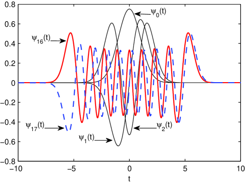
Figure 3: Hermite functions $\psi_{0},\,\psi_{1},\,\psi_{2},\,\psi_{16},\,\psi_{17}$; $\psi_{0}$ is a normalized Gaussian function. Strong decay in time is complemented by the same behaviour in the frequency domain since Hermite functions are eigenfunctions of the Fourier transform.

Since $\{D_{\gamma}\psi_{k};\,k=0,1,\dots\}$ forms a complete orthonormal basis of $L^{2}(\mathbb{R})$, any function $f\in L^{2}(\mathbb{R})$ has an expansion $f(t)=\sum_{k=0}^{\infty}x_{k}\,(D_{\gamma}\psi_{k})(t)$ where the coefficient sequence $x_{0},x_{1},\ldots$ is an element of the space $\ell^{2}(\mathbb{N}_{0})$ of square-summable complex sequences with index set $\mathbb{N}_{0}=\{0,1,\ldots\}$. Hence for any filter input signal $f\in L^{2}(\mathbb{R})$, the filter output signal has the representation

$$(\boldsymbol{P}_{\delta}^{(\gamma)}f)(t)=\sum_{k=0}^{\infty}\rho^{k+\frac{1}{2}}x_{k}\,(D_{\gamma}\psi_{k})(t),$$ (10)

where $x_{k}=\langle f,D_{\gamma}\psi_{k}\rangle$, $\langle f_{1},f_{2}\rangle=\int_{-\infty}^{\infty}f_{1}(t)\overline{f_{2}(t)}\,\mathrm{d}t$ denoting the inner product in $L^{2}(\mathbb{R})$. The new coefficient sequence is $(\rho^{k+\frac{1}{2}}x_{k})_{k=0}^{\infty}$ and again an element of $\ell^{2}(\mathbb{N}_{0})$. Thus, the filter $\boldsymbol{P}_{\delta}^{(\gamma)}$ is reduced to a diagonal linear transformation in $\ell^{2}(\mathbb{N}_{0})$.

In Fig. 3, some Hermite functions are depicted; observe their strong decay in time (and frequency).

2.2 Discretization of the Heat Channel

The perturbed filter output signal is $\tilde{g}(t)=g(t)+n(t)$, where the noise signal $n(t)$ is as described in Def. 1. To extract as much information as possible from $\tilde{g}(t)$ we apply optimal detection (due to North [19]), for example by means of a bank of matched filters [20], in our case LTI filters with impulse response $h_{k}(t)=(D_{\gamma}\psi_{k})(-t)$. When applied to the noisy signal $\tilde{g}(t)$ as input, we get for the matched filter output signals sampled at time zero

$$\int_{-\infty}^{\infty}h_{k}(0-t^{\prime})\tilde{g}(t^{\prime})\,\mathrm{d}t^{\prime}=\rho^{k+\frac{1}{2}}x_{k}+\int_{-\infty}^{\infty}h_{k}(-t^{\prime})n(t^{\prime})\,\mathrm{d}t^{\prime}.$$

From the theory of LTI filters we know that the integral on the RHS evaluates to a realization $n_{k}$ of a zero-mean Gaussian random variable $N_{k}$ with the variance $\theta^{2}\int_{-\infty}^{\infty}h_{k}^{2}(-t)\,\mathrm{d}t$. Since any waveform $D_{\gamma}\psi_{k}$ has $L^{2}$ norm one, the variance of $N_{k}$ is $\theta^{2}$ and, thus, does not depend on $k$. Moreover, because of orthogonality of the waveforms, the random variables $N_{k}$ are independent. Consequently, the detection errors $n_{k}$ are realizations of independent identically distributed ($\mathrm{i.i.d.}$) zero-mean Gaussian random variables $N_{k}\sim\mathcal{N}(0,\theta^{2}),k=0,1,\ldots$. Note that the noise PSD $\theta^{2}$, measured in watts/Hz, has also the dimension of an energy.

Instead of $y_{k}=\rho^{k+\frac{1}{2}}x_{k}$ we now have obtained $\hat{y}_{k}=y_{k}+n_{k}$. So we get the estimate $\hat{x}_{k}=\rho^{-k-\frac{1}{2}}\hat{y}_{k}=x_{k}+z_{k}$ for $x_{k}$, where $z_{k}$ are realizations of independent Gaussian random variables $Z_{k}\sim\mathcal{N}(0,\theta^{2}\rho^{-2k-1}),\,k=0,1,\ldots$. Thus, we are led to the infinite-dimensional vector Gaussian channel

$$Y_{k}=X_{k}+Z_{k},\,k=0,1,\ldots,$$ (11)

where the noise $Z_{k}$ is distributed as described.

$\boldsymbol{X}^{K}=(X_{0},\ldots,X_{K-1})^{T}$ will denote a $K$-dimensional column vector, $K\in\mathbb{N}$, of not necessarily independent random variables $X_{k}$. For any average input energy $S>0$, the vector Gaussian channel consisting of the first $K$ subchannels of the heat channel has capacity [10]

$$C^{K}(S)=\max_{\mathbb{E}\|\boldsymbol{X}^{K}\|^{2}\leq S}I(\boldsymbol{X}^{K};\boldsymbol{Y}^{K}),$$ (12)

where $I(\boldsymbol{X}^{K};\boldsymbol{Y}^{K})$ is the mutual information between random input vector $\boldsymbol{X}^{K}$ and corresponding random output vector $\boldsymbol{Y}^{K}$, $\boldsymbol{X}^{K}$ subject to the average energy constraint $\mathbb{E}\|\boldsymbol{X}^{K}\|^{2}=\sum_{k=0}^{K-1}\mathbb{E}X_{k}^{2}\leq S$. The noise variances $\theta^{2}\rho^{-2k-1},\,k=0,1,\ldots,$ are monotonically increasing and unbounded. Consequently, by reason of the well-known waterfilling argument [11], for any fixed average input energy $S$ the sequence of capacities $C^{1}(S),C^{2}(S),\ldots$ eventually becomes constant. We define

$$C(S)=\lim_{K\rightarrow\infty}C^{K}(S)$$ (13)

as the capacity of the heat channel; $C(S)$ is measured in bits per channel use (or transmission). In Fig. 4, $E_{\mathrm{in}}=S$, the $K$ subchannels to be read in reverse order (as will become clear in Section 3.1); further details of Fig. 4 will be described in the text.

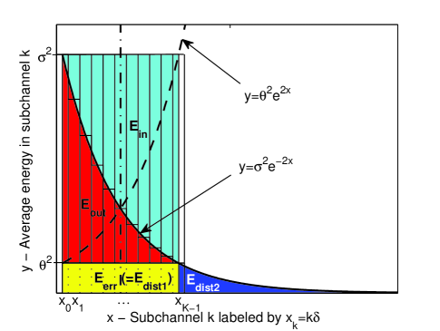
Figure 4: Balance of (average) energies around the heat channel: input/output energy ($E_{\mathrm{in}}/E_{\mathrm{out}}$), energy of measurement error ($E_{\mathrm{err}}$), and distortion ($E_{\mathrm{dist1}}+E_{\mathrm{dist2}}$). Subchannels displayed at distance $\delta\sim\frac{1}{\alpha\beta}$ apart as $\alpha\beta\rightarrow\infty$.

2.3 Example: Dispersion and Amplifier Noise in Fiber Optics

When, as supposed here, in the fiber-optic transmission intensity modulation is applied, real-valued input signals $f\in L^{2}(\mathbb{R})$ need to be replaced by waveforms $\tau_{0}+f(t)$ where $\tau_{0}$ is a fixed positive number chosen large enough so that the resulting signals are nonnegative with high probability [cf. Fig. 9(a), below]. Dispersion is modeled through an LTI filter with impulse response as in (2). The dispersion parameter $\beta=\beta(T)\in(0,\infty)$ in (2) depends on transmission time $T$ as well as the coefficient $a=a(T)\in(0,1]$ in (3) representing attenuation. Then, the fiber output signal is the waveform $a\tau_{0}+u(t)$ where $u(t)$ is given by Eq. (3).

In order to create a heat channel, choose at the receiver any fixed time parameter $\alpha$ with the property that $\alpha>1/\beta$. When the product $\alpha\beta$ is large, the dilation in (7) may be neglected in practice (for simplicity of exposition we imagine of having performed the dilation). Now, apply a variable density neutral filter of appropriate characteristic (an optical device, see [15]) to effect—in the spatial domain—a multiplication of the signal with the time window $w(t)=\exp[-t^{2}/(2\alpha^{2})]$ as shown in (7). Next, amplify the obtained signal by factor $1/a$. When an optical amplifier is employed, the resulting signal is $w_{1}(t)+g(t)+n(t)$ where $w_{1}(t)\propto w(t)$, $g=\boldsymbol{P}_{\delta}^{(\gamma)}f$, and $n(t)$ is a realization of white Gaussian noise (properly modeling the impairment of an optical signal by an optical amplifier; see [7]). After opto electric conversion (possibly adding anew white Gaussian noise to the signal), remove the known signal component $w_{1}(t)$. Finally, use as detection device a bank of matched filters with impulse responses $h_{k}(t),\,k=0,\ldots,K-1,$ as given in Section 2.2; $K$ is a known number depending on the average input energy $S$. Thus, we have implemented a heat channel in an optical fiber communication system.

2.4 Degrees of Freedom of Filter Output Signals

Here, we give an explanation for the time-frequency product $\alpha\beta$ that will occur very frequently in the sequel.

The Wigner-Ville spectrum (WVS) of the response of filter $\boldsymbol{P}_{\delta}^{(\gamma)}$ on white Gaussian noise (see Appendix A for details) is the bivariate function

$$\boldsymbol{\Phi}(t,\omega)=\frac{\sigma^{2}}{2\pi}\cdot\frac{1}{\cosh\delta}\exp\left(-\frac{t^{2}}{\alpha^{2}}-\frac{\omega^{2}}{\beta^{2}}\right).$$ (14)

In general, the WVS of a nonstationary stochastic process gives its density of (average) energy in the time-frequency plane; see, e.g., [29], [28]. Consequently, in our case, the energy of filter output signals would occupy an ellipse-shaped region in the time-frequency plane with unsharp boundary. Regarding the WVS (14) (after a normalization) as a bivariate Gaussian probability density function, we describe this region by an approximation known as ellipse of concentration (EOC) in probability theory [14].

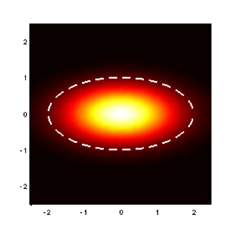
Figure 5: Energy density and EOC (dashed line) for white Gaussian noise response of filter (5) in the limiting case $\alpha\rightarrow\sqrt{2}+,\,\beta\rightarrow(1/\sqrt{2})+$; graphical appearance typical also for other (admissible values) of $\alpha,\beta$.

We obtain as EOC the region $\mathcal{A}_{\mathrm{c}}=\{(t,\omega)\in\mathbb{R}^{2};t^{2}/\alpha^{2}+\omega^{2}/\beta^{2}\leq 2\}$ with area $A_{c}=2\pi\alpha\beta$ [16]. As reported in [12, p. 23], in physics a region in phase space (or time-frequency plane such as here) with area $A$ corresponds to $A/(2\pi)$ “independent states” (when $A$ is sufficiently large). Since here $A_{\mathrm{c}}/(2\pi)=\alpha\beta$, the time-frequency product $\alpha\beta$ would describe the “dimension” of the filter output space (when $\alpha\beta$ is sufficiently large), i.e., the degrees of freedom (DOFs) of filter output signals. In Fig. 5, the energy density in the time-frequency plane as given by the WVS (14) is illustrated.

3 Channel Capacity in Terms of Channel Input, and Optimal Signaling

In this section we derive a closed formula for the capacity of the heat channel in terms of average energy of the channel input signal along with a method of capacity achieving (optimal) signaling. A characterization of channel capacity by waterfilling in the time-frequency plane is also given. The following definition proves to be useful.

Definition 2.

For any two functions $A,\,B:(1,\infty)\rightarrow\mathbb{R}$ the notation $A\doteq B$ means

$$\lim_{x\rightarrow\infty}\frac{A(x)-B(x)}{x}=0,$$

or, equivalently, $A(x)=B(x)+o(x)$ as $x\rightarrow\infty$.

In our context, $x$ will always be the time-frequency product $\alpha\beta>1$. Thus, $A\doteq B$ implies that $A(\alpha\beta)/(\alpha\beta)=B(\alpha\beta)/(\alpha\beta)+\epsilon$ where $\epsilon\rightarrow 0$ as $\alpha\beta\rightarrow\infty$.

3.1 Channel Capacity in Closed Form

The function $y=w_{0}(x),\,x\geq 0,$ occurring in the next theorem is the inverse function of $y=(2x-1)e^{2x}+1,\,x\geq 0$ (see also Fig. 6).

Theorem 1.

Assume that the average energy $S$ of the input signal depends on $\alpha\beta$ such that $S(\alpha\beta)=O(\alpha\beta)$ as $\alpha\beta\rightarrow\infty$. Then for the capacity (in bits per transmission) of the heat channel it holds

$$C(S)\doteq\frac{\alpha\beta}{2}\left[w_{0}\left(\frac{S}{(\alpha\beta/2)\theta^{2}}\right)\right]^{2}\log_{2}e.$$ (15)

Proof:.

The proof is accomplished by waterfilling [8, Th. 7.5.1], [11]. Let $\nu_{k}^{2}=\theta^{2}\rho^{-2k-1},\,k=0,1,\ldots,$ be the variance of noise in the $k$th subchannel of the discetized heat channel (11). The positive number $\sigma$ is defined by the condition

$$S=\sum_{k=0}^{\infty}(\sigma^{2}-\nu_{k}^{2})^{+}=\sum_{k=0}^{K-1}(\sigma^{2}-\nu_{k}^{2}),$$ (16)

where $x^{+}\triangleq\max\{0,x\},\,x\in\mathbb{R},$ and $K=\max\{k\in\mathbb{N};\nu_{k-1}^{2}<\sigma^{2}\}$ is the number of subchannels in the resulting finite-dimensional vector Gaussian channel. With increasing time-frequency product $\alpha\beta$, $\delta=\delta(\alpha\beta)$ (now acting as increment) tends to 0 so that

$$S\cdot\delta = \sum_{k=0}^{K-1}(\sigma^{2}-\theta^{2}e^{2k\delta}e^{\delta})\delta$$ (17)

$$= \int_{0}^{\infty}(\sigma^{2}-\theta^{2}e^{2x})^{+}\,\mathrm{d}x+\epsilon,$$

where $\epsilon\rightarrow 0$ as $\alpha\beta\rightarrow\infty$. Observe that by the growth condition imposed on $S=S(\alpha\beta)$ and because of $\delta\sim\frac{1}{\alpha\beta}$, it holds $\limsup_{\alpha\beta\rightarrow\infty}S\cdot\delta<\infty$ so that transition to a Riemann integral is allowed; for later reference still note that the water level $\sigma^{2}=\sigma^{2}(\alpha\beta)$ also remains bounded as $\alpha\beta\rightarrow\infty$. Evaluation of the integral yields

$$S\doteq\frac{\alpha\beta}{2}\theta^{2}\cdot\left(\frac{\sigma^{2}}{\theta^{2}}\ln\frac{\sigma^{2}}{\theta^{2}}-\frac{\sigma^{2}}{\theta^{2}}+1\right).$$ (18)

The maximum in Eq. (12) is achieved when the components $X_{k}$ of the input vector $\boldsymbol{X}^{K}$ are independent $\sim\mathcal{N}(0,\sigma^{2}-\nu_{k}^{2})$ and the capacity (in nats) becomes

$$C=C(S)=\sum_{k=0}^{K-1}\frac{1}{2}\ln\left(1+\frac{\sigma^{2}-\nu_{k}^{2}}{\nu_{k}^{2}}\right).$$ (19)

Since $\sigma^{2}$ eventually remains bounded, transition to a Riemann integral in the next equations is allowed and we get

$$C\cdot\delta = \sum_{k=0}^{K-1}\frac{1}{2}\ln\left(\frac{\sigma^{2}}{\theta^{2}}e^{-2k\delta}e^{-\delta}\right)\delta$$

$$= \int_{0}^{\infty}\left[\frac{1}{2}\ln\left(\frac{\sigma^{2}}{\theta^{2}}e^{-2x}\right)\right]^{+}\,\mathrm{d}x+\epsilon$$

$$= \frac{1}{2}\left(\frac{1}{2}\ln\frac{\sigma^{2}}{\theta^{2}}\right)^{2}+\epsilon,$$

where $\epsilon\rightarrow 0$ as $\alpha\beta\rightarrow\infty$. Thus it holds

$$C\doteq\frac{\alpha\beta}{2}\left(\frac{1}{2}\ln\frac{\sigma^{2}}{\theta^{2}}\right)^{2}.$$ (20)

Eq. (18) is equivalent to

$$\frac{\sigma^{2}}{e\theta^{2}}\ln\frac{\sigma^{2}}{e\theta^{2}}=e^{-1}(s-1)+\epsilon_{1},$$

where $s=S/[(\alpha\beta/2)\theta^{2}]$ and $\epsilon_{1}\rightarrow 0$ as $\alpha\beta\rightarrow\infty$. By means of the Lambert $W$ function [22] (actually its principal branch $W_{0}$, see Fig. 6) which is the uniquely determined analytic function satisfying $W(x)\exp[W(x)]=x\>\>\mbox{for all}\>\>x\in[-e^{-1},\infty)$ and $W(0)=0$, we get after a computation

$$\frac{1}{2}\left(\frac{1}{2}\ln\frac{\sigma^{2}}{\theta^{2}}\right)^{2}=\frac{1}{2}\left[w_{0}(s+\epsilon_{1}^{\prime})\right]^{2},$$

where we have put $w_{0}(x)=\frac{1}{2}[1+W((x-1)/e)],\,x\geq 0$, and $\epsilon_{1}^{\prime}=e\epsilon_{1}$.

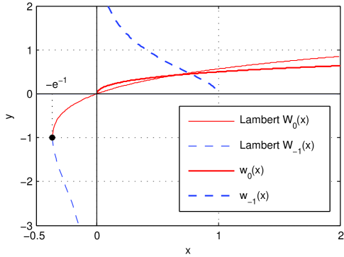
Figure 6: Lambert $W$ function: branches $W_{0}(x),\,W_{-1}(x)$ and related functions $w_{0}(x),\,w_{-1}(x).$

Because of Eq. (20), this gives rise to

$$\frac{C}{\alpha\beta}=\frac{1}{2}\left[w_{0}(s+\epsilon_{1}^{\prime})\right]^{2}+\epsilon_{2},$$

where $\epsilon_{2}\rightarrow 0$ as $\alpha\beta\rightarrow\infty$. Unlike $w_{0}(x)$, which has a vertical tangent at $x=0$, the function $(w_{0}(x))^{2}$ has a continuous and bounded derivative in every closed interval $[0,s_{0}]\subset[0,\infty)$. Consequently, by the mean value theorem we obtain $C/(\alpha\beta)=\frac{1}{2}\left[w_{0}(s)\right]^{2}+\epsilon_{1}^{\prime\prime}+\epsilon_{2}$ where $\epsilon_{1}^{\prime\prime}+\epsilon_{2}\rightarrow 0$ as $\alpha\beta\rightarrow\infty$. After transition from nats to bits ($1\>\mbox{nat}=\log_{2}\!e\>\>\mbox{bit}$), Eq. (15) is obtained. ∎

We discuss the case $0<S=S(\alpha\beta)\propto\alpha\beta$ in more detail. First, if $\beta>0$ is held constant, then $S=\alpha\beta S_{1}=2\pi\alpha P,\,P=\beta S_{1}/(2\pi)$. Suppose that an individual input signal has maximum duration $2\pi\alpha$ (cf. Fig. 9) and signals are sent every time $2\pi\alpha$. Then no ISI occurs and the capacity is approximately $C(S)/(2\pi\alpha)$, where $C(S)$ is given by the dotted Eq. (15); forming the limit $\bar{C}\triangleq\lim_{\alpha\rightarrow\infty}C(S)/(2\pi\alpha)$ turns Eq. (15) into the true equation

$$\bar{C}=\frac{1}{2\pi}\frac{\beta}{2}\left[w_{0}\left(2\pi\frac{P}{(\beta/2)\theta^{2}}\right)\right]^{2}\log_{2}e\quad\mbox{(bit/s).}$$ (21)

Next, let $\beta\rightarrow\infty$. Since $w_{0}(0)=0$ and $(w_{0}(x))^{2}$ is differentiable at $x=0$ with derivative $1/2$, it follows that

$$\bar{C}\rightarrow\frac{P}{2\theta^{2}}\log_{2}e\>\>\mbox{(bit/s)}.$$ (22)

Finally, we compare (21) with the capacity of the bandlimited Gaussian channel of bandwidth $W$ and one-sided noise PSD $N_{0}$ given by Shannon’s classic formula [10]

$$C=W\log_{2}\left(1+\frac{P}{WN_{0}}\right)\>\>\mbox{(bit/s)}.$$ (23)

Rewrite the latter equation as $C(\mathrm{SNR})=W\log_{2}(1+\mathrm{SNR})$ where $\mathrm{SNR}=P/(WN_{0})$. In case of the heat channel, it is consistent to put $\mathrm{SNR}=P/(WN_{0})$ where $W=\beta/2$, $N_{0}=2\theta^{2}$ is the one-sided noise PSD, and to rewrite Eq. (21) as $C(\mathrm{SNR})=(2\pi)^{-1}W\,\left[w_{0}\left(4\pi\,\mathrm{SNR}\right)\right]^{2}\log_{2}e$. In Figs. 7 and 8, the corresponding spectral efficiencies $C(\mathrm{SNR})/W$ are plotted as a function of SNR or $E_{\mathrm{b}}/N_{0}$, respectively. Although the spectral efficiency of the heat channel rapidly falls behind that of the bandlimited Gaussian channel, we observe that the capacity limit in (22) is exactly the same as for a Gaussian channel with infinite bandwidth, average input power $P$ and one-sided noise PSD $N_{0}=2\theta^{2}$; cf. [11, Eq. (9.63)].

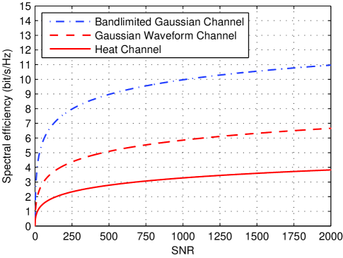
Figure 7: Spectral efficiencies of heat channel, bandlimited Gaussian channel, and Gaussian waveform channel as a function of SNR.

Figure 8: Spectral efficiencies of heat channel, bandlimited Gaussian channel, and Gaussian waveform channel plotted against $10\log_{10}E_{\mathrm{b}}/N_{0}$, where $E_{\mathrm{b}}$ is average input energy per bit and $N_{0}$ is one-sided noise PSD of the AWGN.

3.2 Optimal Signaling for the Continuous-Time Channel

We return to our original model of the heat channel as given in Def. 1. For a fixed average input energy $S>0$ and noise PSD $\theta^{2}>0$, the capacity achieving (optimal) input signals are now waveforms

$$f(t)=\sum_{k=0}^{K-1}x_{k}\,(D_{\gamma}\psi_{k})(t),\,t\in\mathbb{R},$$ (24)

where the coefficients $x_{k}$ are realizations of independent Gaussian random variables $X_{k}\sim\mathcal{N}(0,\sigma^{2}-\nu_{k}^{2}),k=0,\ldots,K-1,$ as in the proof of Th. 1. The corresponding (“optimal”) filter output signals are

$$g(t)=\sum_{k=0}^{K-1}y_{k}\,(D_{\gamma}\psi_{k})(t),\,t\in\mathbb{R},$$ (25)

where the coefficients $y_{k}=\rho^{k+\frac{1}{2}}x_{k}$ are realizations of independent Gaussian random variables $Y_{k}\sim\mathcal{N}(0,\sigma_{k}^{2}-\theta^{2})$, $\sigma_{k}^{2}=\sigma^{2}\rho^{2k+1},k=0,\ldots,K-1$.

The following numerical example may serve as illustration. In Fig. 9, a pair of optimal filter input/output signals is depicted. Since transmission through an optical fiber by intensity modulation is supposed, the input signal $f(t)$ is modified as described in Section 2.3. By means of Eq. (15), the capacity is found to be approximately 64.75 bits per transmission (numerical computation gives the exact value of 64.59). Since the effective duration of the fiber input signal is less than $2\pi\alpha=0.3141\,\mathrm{ns}$, a sequence of such random pulses sent every time $2\pi\alpha$ would transmit approximately 206.1 Gbit/s—in contrast to 50 Gbit/s as inferred from (4). In the present example, $K=30$ coefficients per waveform are needed.

Now, let $\alpha\beta\rightarrow\infty$. Under the assumption of Th. 1, the number $K$ of coefficients (or active subchannels) is found to be

$$K\doteq\frac{\alpha\beta}{2}\ln\frac{\sigma^{2}}{\theta^{2}}\>.$$ (26)

For the sake of simplicity, assume further that $0<S(\alpha\beta)\propto\alpha\beta$. Then, by (17), we infer that $\sigma^{2}$ approaches a finite water level $\bar{\sigma}^{2}>\theta^{2}$ as $\alpha\beta\rightarrow\infty$. As a consequence, $K\rightarrow\infty$ and $\sigma_{k}^{2}-\theta^{2}\rightarrow\bar{\sigma}_{k}^{2}-\theta^{2}$ where we have put $\bar{\sigma}_{k}^{2}=\bar{\sigma}^{2}\rho^{2k+1}$. When $\bar{\sigma}^{2}$ is large compared to $\theta^{2}$, the bias $\theta^{2}$ in $\bar{\sigma}_{k}^{2}-\theta^{2}$ may be neglected so that the optimal filter output signal (25) comes close to a white Gaussian noise response; cf. (32) (below) and Appendix A. Then, the signal model of Section 2.4 is almost met and we may take (and shall do so in the sequel) the time-frequency product $\alpha\beta$ as DOFs of optimal filter output signals.

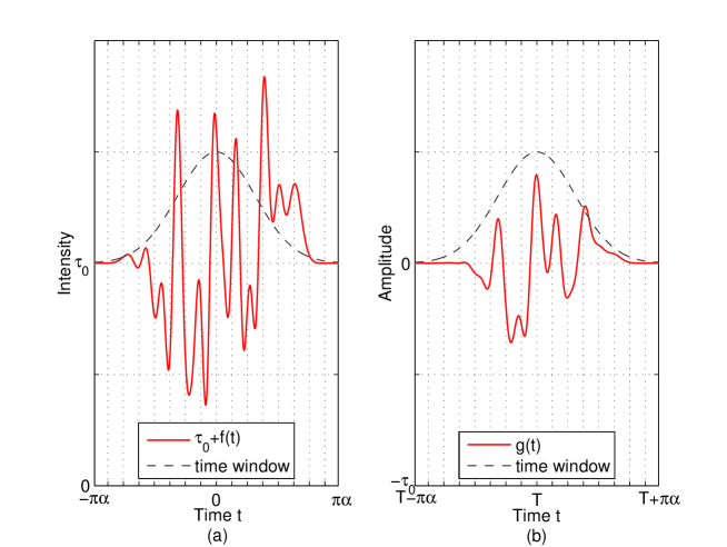
Figure 9: Optimal waveforms for the heat channel with parameters $\alpha=50\,\mathrm{ps},\,\beta=200\,\mathrm{GHz},\,\mathrm{SNR}=159.1(\approx 1000/2\pi)$.; time window refers to Gaussian prefactor in (5). (a) Physical input signal $\tau_{0}+f(t)$ to an optical fiber. (b) Corresponding filter output signal $g(t)$ after transmission time $T$.

3.3 Waterfilling Theorem for the Heat Channel

By means of a Szegő theorem (namely Th. 7 in Appendix B), the above waterfilling solution carries over to the time-frequency plane. The classic waterfilling solution for the capacity of a power-constraint additive Gaussian noise channel goes back to Shannon [33] and has been stated and proved by Gallager [8] in full generality.

Referring to Gallager’s capacity theorem [8, Th. 8.5.1] in the form given in [11, (9.97)], we define

$$N(t,\omega)=\frac{\theta^{2}}{2\pi}\cdot(\cosh\delta)\exp\left(\frac{t^{2}}{\alpha^{2}}+\frac{\omega^{2}}{\beta^{2}}\right).$$

Now we are in a position to state

Theorem 2.

Under the same assumption on the average input energy $S$ as in Th. 1, the capacity (in bits per transmission) of the heat channel is given by

$$C\doteq\frac{1}{2\pi}\int\!\!\!\int_{\mathbb{R}^{2}}\frac{1}{2}\log_{2}\left(1+\frac{(\nu-N(t,\omega))^{+}}{N(t,\omega)}\right)\,\mathrm{d}t\,\mathrm{d}\omega,$$ (27)

where $\nu$ is chosen so that

$$S\doteq\int\!\!\!\int_{\mathbb{R}^{2}}(\nu-N(t,\omega))^{+}\,\mathrm{d}t\,\mathrm{d}\omega.$$ (28)

Proof:.

See Appendix B. ∎

Note that the bivariate function $N(t,\omega)$ is proportional to the reciprocal WVS $\boldsymbol{\Phi}(t,\omega)$ in (14). Since $N(t,\omega)$ has the form of a “cup,” Th. 2 is a waterfilling theorem in a very real sense.

When $\alpha\rightarrow\infty$, the time-varying heat channel appears [34] to tend towards an (LTI) waveform channel according to Gallager’s model with LTI filter with Gaussian impulse response (2) (we shall call it Gaussian waveform channel). It is therefore interesting to compare Th. 2 with [8, Th. 8.5.1] when applied to that particular waveform channel (with AWGN of noise PSD $N_{0}/2=\theta^{2}$). According to Gallager’s theorem, the capacity $C$ (in bits per second) for input power $S$ is given parametrically by (we stick to the notations in [8])

$$C = \int_{-\infty}^{\infty}\frac{1}{2}\left[\log_{2}\frac{|H_{1}(f)|^{2}B}{N_{0}/2}\right]^{+}\,\mathrm{d}f$$

$$S = \int_{-\infty}^{\infty}\left[B-\frac{N_{0}/2}{|H_{1}(f)|^{2}}\right]^{+}\,\mathrm{d}f,$$

where $H_{1}(f)=\int_{-\infty}^{\infty}e^{-2\pi ift}h_{1}(t)\,\mathrm{d}t$ is the frequency response of the filter. For the function $h_{1}(t)$ at hand, we obtain

$$C = \frac{1}{2\pi}\int_{-\infty}^{\infty}\frac{1}{2}\log_{2}\left(1+\frac{(\nu-N_{1}(\omega))^{+}}{N_{1}(\omega)}\right)\,\mathrm{d}\omega$$ (29)

$$S = \int_{-\infty}^{\infty}(\nu-N_{1}(\omega))^{+}\,\mathrm{d}\omega,$$ (30)

where $\nu$ is the parameter, $\omega$ is angular frequency, and

$$N_{1}(\omega)=\frac{\theta^{2}}{2\pi}\cdot\exp\left(\frac{\omega^{2}}{\beta^{2}}\right).$$ (31)

We observe perfect formal analogy between the waterfilling formulas (29), (30) and those in Th. 2. Moreover, $N(t,\omega)$ tends to $N_{1}(\omega)$ as $\alpha\rightarrow\infty$ for any $t,\omega$ held constant. In Figs. 7 and 8, the spectral efficiency $C/W$ of the Gaussian waveform channel is plotted as a function of SNR or $E_{\mathrm{b}}/N_{0}$, respectively.

4 Rate Distortion Function for a Related Nonstationary Source

For a well-rounded treatment of the capacity problem for the heat channel it is expedient to investigate a dual problem, which is a topic of rate distortion theory. To this end, consider the nonstationary source given by the nonstationary zero-mean Gaussian process defined by the Karhunen-Loève expansion

$$X(t)=\sum_{k=0}^{\infty}X_{k}\,(D_{\gamma}\psi_{k})(t),\,t\in\mathbb{R},$$ (32)

where the coefficients $X_{k},\,k=0,1,\ldots,$ are independent Gaussian random variables $\sim\mathcal{N}(0,\sigma_{k}^{2})$ of variance $\sigma_{k}^{2}=\sigma^{2}\rho^{2k+1},\,\sigma>0$. It is the response of filter $\boldsymbol{P}_{\delta}^{(\gamma)}$ on white Gaussian noise; cf. (53) in Appendix A. In Fig. 4, the area beneath the curve $y=\sigma^{2}e^{-2x}$ corresponds to the average energy

$$E=\sum_{k=0}^{\infty}\sigma_{k}^{2}=\frac{\sigma^{2}\rho}{1-\rho^{2}}\doteq\frac{\alpha\beta}{2}\sigma^{2}$$ (33)

of the Gaussian process (32). The parameter $\theta^{2}$ in Fig. 4 will now have the interpretation of a “(ground-)water table.” In this section, information will be measured in nats.

4.1 Rate Distortion Function in Closed Form

Substitute the continuous-time Gaussian process $\{X(t),\,t\in\mathbb{R}\}$ in (32) by the sequence of coefficient random variables $\boldsymbol{X}=X_{0},X_{1},\ldots\,$. For an estimate $\boldsymbol{\hat{X}}=\hat{X}_{0},\hat{X}_{1},\ldots$ of $\boldsymbol{X}$ we take the mean-square error $D=\mathbb{E}\{\sum_{k=0}^{\infty}(X_{k}-\hat{X}_{k})^{2}\}$ as distortion measure.

The function $y=w_{-1}(x),\,0<x\leq 1,$ occurring in the next theorem is the inverse function of $y=(2x+1)e^{-2x},\,x\geq 0$ (see also Fig. 6). The Landau symbol $\Omega(\cdot)$ is defined for any two functions as in Def. 2 as follows: $A(x)=\Omega(B(x))$ as $x\rightarrow\infty$ if $B(x)>0$ and $\liminf_{x\rightarrow\infty}A(x)/B(x)>0$.

Theorem 3.

Assume that the foregoing average distortion $D$ depends on $\alpha\beta$ such that $D(\alpha\beta)=\Omega(\alpha\beta)$ as $\alpha\beta\rightarrow\infty$. Then the rate distortion function for the nonstationary source (32) satisfies

$$R(D)\doteq\frac{\alpha\beta}{2}\left[w_{-1}\left(\frac{D}{(\alpha\beta/2)\sigma^{2}}\right)\right]^{2}$$ (34)

if $D\leq(\alpha\beta/2)\sigma^{2}$, and $R(D)\doteq 0$ otherwise. The rate is measured in nats per realization of the source.

Proof:.

Let $E$ be the average energy (33) of the Gaussian process (32).

First, assume $D\leq E$. The reverse waterfilling argument for a finite number of independent Gaussian sources [11] carries over to our case without changes resulting in a finite collection of Gaussian sources $X_{0},\ldots,X_{K-1}$ where $K=\max\{k\in\mathbb{N};\sigma_{k-1}^{2}>\theta^{2}\}$ and the water level $\theta^{2}>0$ is defined by the condition

$$D=\sum_{k=0}^{\infty}\min\{\theta^{2},\sigma_{k}^{2}\},$$ (35)

(cf. Fig. 4, where $D=E_{\mathrm{dist1}}+E_{\mathrm{dist2}}$). Consequently,

$$D\cdot\delta = \sum_{k=0}^{\infty}\min\{\theta^{2},\sigma^{2}e^{-2k\delta}e^{-\delta}\}\delta$$ (36)

$$= \int_{0}^{\infty}\min\{\theta^{2},\sigma^{2}e^{-2x}\}\,\mathrm{d}x+\epsilon,$$

where $\epsilon\rightarrow 0$ as $\alpha\beta\rightarrow\infty$. Observe that by the growth condition imposed on $D$ and since $\delta\sim\frac{1}{\alpha\beta}$, the water level $\theta^{2}$ eventually remains above a positive lower bound as $\alpha\beta\rightarrow\infty$. Evaluation of the integral yields

$$D\doteq\frac{\alpha\beta}{2}\sigma^{2}\cdot\left(\frac{\theta^{2}}{\sigma^{2}}-\frac{\theta^{2}}{\sigma^{2}}\ln\frac{\theta^{2}}{\sigma^{2}}\right).$$ (37)

The rate distortion function is parametrically given by [11]

$$R=\sum_{k=0}^{K-1}\frac{1}{2}\ln\frac{\sigma_{k}^{2}}{\theta^{2}}.$$ (38)

The RHSs of Eqs. (38) and (19) agree. Since $\frac{1}{\theta^{2}}$ is eventually finitely upper bounded, transition to a Riemann integral is allowed and we obtain exactly as in the proof of (20) that

$$R\doteq\frac{\alpha\beta}{2}\left(\frac{1}{2}\ln\frac{\sigma^{2}}{\theta^{2}}\right)^{2}.$$ (39)

Eq. (37) is equivalent to

$$\frac{\theta^{2}}{e\sigma^{2}}\ln\frac{\theta^{2}}{e\sigma^{2}}=-e^{-1}d+\epsilon_{1},$$

where $d=D/[(\alpha\beta/2)\sigma^{2}]$ and $\epsilon_{1}\rightarrow 0$ as $\alpha\beta\rightarrow\infty$. By means of the branch $W_{-1}$ of the Lambert $W$ function [22], which is the uniquely determined analytic function satisfying $W_{-1}(x)\exp[W_{-1}(x)]=x\>\>\mbox{for all}\>\>x\in[-e^{-1},0)$ and $W_{-1}(-e^{-1})=-1,\,W_{-1}(x)\rightarrow-\infty$ as $x\rightarrow 0-$ (see Fig. 6), we get after a computation

$$\frac{1}{2}\left(\frac{1}{2}\ln\frac{\sigma^{2}}{\theta^{2}}\right)^{2}=\frac{1}{2}\left[w_{-1}(d+\epsilon_{1}^{\prime})\right]^{2},$$

where we have put $w_{-1}(x)=\frac{1}{2}[-1-W_{-1}(-x/e)],\,0<x\leq 1$, and $\epsilon_{1}^{\prime}=-e\epsilon_{1}$. Because of Eq. (39), this gives rise to

$$\frac{R}{\alpha\beta}=\frac{1}{2}\left[w_{-1}(d+\epsilon_{1}^{\prime})\right]^{2}+\epsilon_{2},$$

where $\epsilon_{2}\rightarrow 0$ as $\alpha\beta\rightarrow\infty$. Unlike $w_{-1}(x)$, which has a vertical tangent at $x=1$, the function $(w_{-1}(x))^{2}$ has a continuous and bounded derivative in any closed interval $[d_{0},1]\subset(0,1]$. Consequently, by the mean value theorem $R/(\alpha\beta)=\frac{1}{2}\left[w_{-1}(d)\right]^{2}+\epsilon_{1}^{\prime\prime}+\epsilon_{2}$ where $\epsilon_{1}^{\prime\prime}+\epsilon_{2}\rightarrow 0$ as $\alpha\beta\rightarrow\infty$ uniformly for all $d\in[d_{0},1]$. This proves the first part of the theorem.

Now, suppose that $D>E$. Since $\mathbb{E}\{\sum_{k=0}^{\infty}(X_{k}-0)^{2}\}=E<D$, the constant sequence $\boldsymbol{\hat{X}}=0,0,\ldots$ is a sufficient estimate. Since there is no uncertainty about the members of that deterministic sequence, no information needs to be supplied; thus, $R=0$. This proves the second part of the theorem. ∎

4.2 Reverse Waterfilling in the Time-Frequency Plane

Before continuing with our main theme, we present a parametric representation of the rate distortion function occurring in Th. 3 since the means for its proof—Th. 7 in Appendix B—are now available. This representation may be viewed as an extension to the time-frequency plane of the classic method of reverse waterfilling (cf., e.g., [31], [11]) due to Kolmogorov [30]. It turns out that the part of the PSD in [31, Th. 4.5.4] is now taken by the WVS $\boldsymbol{\Phi}(t,\omega)$ in (14). We obtain

Theorem 4.

The rate distortion function $R(D)$ for the nonstationary source (32) has in the interval $0<D\leq(\alpha\beta/2)\sigma^{2}$ the parametric representation

$$R_{\lambda} \doteq \frac{1}{2\pi}\int\!\!\!\int_{\mathbb{R}^{2}}\max\left\{0,\frac{1}{2}\ln\frac{\boldsymbol{\Phi}(t,\omega)}{\lambda}\right\}\,\mathrm{d}t\,\mathrm{d}\omega$$

$$D_{\lambda} \doteq \int\!\!\!\int_{\mathbb{R}^{2}}\min\left\{\lambda,\boldsymbol{\Phi}(t,\omega)\right\}\,\mathrm{d}t\,\mathrm{d}\omega.$$

Proof:.

See Appendix B. ∎

Note that

$$\int\!\!\!\int_{\mathbb{R}^{2}}\boldsymbol{\Phi}(t,\omega)\,\mathrm{d}t\,\mathrm{d}\omega=\frac{\alpha\beta}{2}\frac{\sigma^{2}}{\cosh\delta}\doteq\frac{\alpha\beta}{2}\sigma^{2}$$

is the average energy (33) of the nonstationary Gaussian process (32) (as it should be). We observe that the representation in Th. 4 is in perfect analogy to the parametric representation [31, Eqs. (4.5.51), (4.5.52)] of the $R(D)$ function for a continuous-time stationary Gaussian source.

5 Channel Capacity in Terms of Channel Output, and Relation to Detection Theory

Now, we adopt the perspective of the receiver. This will result in a second closed-form capacity formula for the heat channel, now in terms of elementary functions and akin to the classic Shannon formula (23) for the capacity of a bandlimited Gaussian channel. Moreover, we shall find a parallel to the well-known I-MMSE relationship [32]. Implications for the capacity of multiple-input multiple-output (MIMO) systems will be indicated. In the present section, it is convenient to use natural logarithms; therefore, information is measured in nats.

5.1 Channel Capacity—Second Formula in Closed Form

For any fixed average input energy $S$ the capacity achieving input signals to the continuous-time heat channel are waveforms $f(t)=\sum_{k=0}^{K-1}x_{k}\,(D_{\gamma}\psi_{k})(t)$, where the coefficients $x_{k}$ are realizations of independent Gaussian random variables $X_{k}\sim\mathcal{N}(0,\sigma^{2}-\nu_{k}^{2})$ (where $K$, $\sigma$ and $\nu_{k}$ are same as in the proof of Th. 1). In the next theorem, the capacity of the heat channel will be expressed in terms of the average energy $\hat{E}_{\mathrm{out}}$ of the detected perturbed filter output signal $\hat{g}(t)=\sum_{k=0}^{K-1}\hat{y}_{k}\,(D_{\gamma}\psi_{k})(t)$, or rather its coefficients $\hat{y}_{k}=\rho^{k+\frac{1}{2}}x_{k}+n_{k}$ obtained by optimal detection (through matched filters). Then the detection errors $n_{k}$ are realizations of $\mathrm{i.i.d.}$ random variables $N_{k}\sim\mathcal{N}(0,\theta^{2})$ as in Section 2.

Theorem 5.

Assume that the average energy $\hat{E}_{\mathrm{out}}$ of the detected perturbed filter output signal depends on $\alpha\beta$ such that $\hat{E}_{\mathrm{out}}(\alpha\beta)=O(\alpha\beta)$ as $\alpha\beta\rightarrow\infty$. Then the capacity (in nats per transmission) of the heat channel is given by

$$C\doteq\frac{\alpha\beta}{2}\left[\ln\sqrt{1+\frac{\hat{E}_{\mathrm{out}}}{(\alpha\beta/2)\theta^{2}}}\,\right]^{2}.$$ (40)

Proof:.

Rewrite Eq. (20) as

$$C\doteq\frac{\alpha\beta}{2}\left[\ln\sqrt{1+\frac{(\alpha\beta/2)(\sigma^{2}-\theta^{2})}{(\alpha\beta/2)\theta^{2}}}\,\right]^{2}$$ (41)

and put $\sigma_{k}^{2}=\sigma^{2}\rho^{2k+1},\,k=0,1,\ldots\,$. In case of capacy achieving (optimal) signaling, the average energy of the detected perturbed filter output signal is $\hat{E}_{\mathrm{out}}=E_{\mathrm{out}}+E_{\mathrm{err}}$ (cf. Fig. 4) where $E_{\mathrm{out}}=\sum_{k=0}^{K-1}(\sigma_{k}^{2}-\theta^{2})$ is the average energy of the filter output signal, $E_{\mathrm{err}}=\sum_{k=0}^{K-1}\theta^{2}$ is the average energy of the (total) detection error, and $K$ is given by $K=\max\{k\in\mathbb{N};\sigma_{k-1}^{2}>\theta^{2}\}$ (coinciding with the number $K$ of active subchannels in the proof of Th. 1). Since $\hat{E}_{\mathrm{out}}=\sum_{k=0}^{K-1}\sigma_{k}^{2}$ and $\delta\sim\frac{1}{\alpha\beta}\,(\alpha\beta\rightarrow\infty)$, we get

$$\hat{E}_{\mathrm{out}}\cdot\delta=e^{-\delta}\sum_{k=0}^{K-1}\sigma^{2}e^{-2k\delta}\delta=\int_{0}^{\frac{1}{2}\ln\frac{\sigma^{2}}{\theta^{2}}}\sigma^{2}e^{-2x}\,\mathrm{d}x+\epsilon=\frac{1}{2}(\sigma^{2}-\theta^{2})+\epsilon,$$

where $\epsilon\rightarrow 0$ as $\alpha\beta\rightarrow\infty$. Observe that by the growth condition imposed on $\hat{E}_{\mathrm{out}}$, $\sigma^{2}$ remains bounded as $\alpha\beta\rightarrow\infty$ (justifying in hindsight the transition to a Riemann integral). Hence,

$$\hat{E}_{\mathrm{out}}\doteq\frac{\alpha\beta}{2}(\sigma^{2}-\theta^{2}).$$ (42)

Now Eq. (40) follows from Eqs. (41), (42). ∎

Note that for the determination of channel capacity by formula (40), the receiver does not need to know the number $K$ of active subchannels beforehand, since, at least in principle, it could easily be estimated as accurately as desired from successive optimal channel uses at constant average input energy.

In the rest of this section we shall always suppose that $K$ is given by Eq. (26), tacitly assuming that the assumptions of Th. 1 (or Th. 5) are fulfilled.

5.2 A C-NODE Relationship

The setting of the previous subsection gives rise to a vector Gaussian channel

$$\boldsymbol{Y}^{K}=\boldsymbol{H}^{K}\boldsymbol{X}^{K}+\boldsymbol{N}^{K},$$ (43)

where the matrix $\boldsymbol{H}^{K}$ is the $K\times K$ diagonal matrix with entries $h_{kk}=\rho^{k+\frac{1}{2}},\,k=0,\ldots,K-1$, $\boldsymbol{X}^{K}$ is a random input vector satisfying $\mathbb{E}\|\boldsymbol{X}^{K}\|<\infty$, and the noise vector $\boldsymbol{N}^{K}$ has independent random components $N_{k}\sim\mathcal{N}(0,\theta^{2})$. Recall that the noise is caused by errors coming from optimal detection. The noise has average energy $\mathbb{E}\|\boldsymbol{N}^{K}\|^{2}$; we define the normalized optimal detection error (NODE) as

$$\mathrm{node}(S)=\frac{\mathbb{E}\|\boldsymbol{N}^{K}\|^{2}}{\sigma^{2}}=\frac{K\theta^{2}}{\sigma^{2}}$$ (44)

where $S$ is the average energy of channel input signals (or vectors) and $\sigma^{2}$ is determined by Eq. (16). Because of Eq. (26), it holds that

$$\mathrm{node}(S)\doteq\frac{\alpha\beta}{2}\frac{\theta^{2}}{\sigma^{2}}\ln\frac{\sigma^{2}}{\theta^{2}}$$ (45)

The quantity $\mathrm{node}(S)$ is called normalized because $\mathbb{E}\|\boldsymbol{N}^{K}\|^{2}=K\theta^{2}\doteq\frac{\alpha\beta}{2}\theta^{2}\ln\frac{\sigma^{2}}{\theta^{2}}$ turns into the RHS of Eq. (45) after rescaling $\sigma,\theta\leftarrow 1,\theta/\sigma$. Notice that the NODE as defined in (44) is physically dimensionless.

5.2.1 Motivation and Derivation

The central result of [32] is an identity connecting mutual information with the minimum mean-square error (MMSE) of estimation theory (I-MMSE relationship); it reads

$$\frac{\mathrm{d}}{\mathrm{d}\,\mathrm{snr}}I(\boldsymbol{X};\sqrt{\mathrm{snr}}\boldsymbol{H}\boldsymbol{X}+\boldsymbol{N})=\frac{1}{2}\mathrm{mmse}(\mathrm{snr}),$$ (46)

where $\boldsymbol{N}$ is a noise vector with independent standard Gaussian components, independent of the random vector $\boldsymbol{X}$, $\mathbb{E}\|\boldsymbol{X}\|^{2}<\infty$, and $\boldsymbol{H}$ is a deterministic matrix of appropriate dimension. It is interesting to compare Eq. (46) with the capacity calculations in our paper. We shall denote the inverse matrix of $\boldsymbol{H}^{K}$ by $\boldsymbol{H}^{-K}$. Since mutual information is invariant with respect to invertible linear transformations, we infer for the mutual information $I(\boldsymbol{X}^{K};\boldsymbol{Y}^{K})=I(\boldsymbol{X}^{K};\boldsymbol{X}^{K}+\boldsymbol{H}^{-K}\boldsymbol{N}^{K})$ occurring in Eq. (12) that

$$I(\boldsymbol{X}^{K};\boldsymbol{Y}^{K})=I\left(\boldsymbol{X}^{\prime K};\frac{\sigma}{\theta}\boldsymbol{H}^{K}\boldsymbol{X}^{\prime K}+\boldsymbol{N}^{\prime K}\right).$$ (47)

where the noise vector $\boldsymbol{N}^{\prime K}=\theta^{-1}\boldsymbol{N}^{K}$ has independent standard Gaussian components, independent of the random vector $\boldsymbol{X}^{\prime K}=\sigma^{-1}\boldsymbol{X}^{K}$. If we take in (47) for $\boldsymbol{X}^{\prime K}=(X^{\prime}_{0},\ldots,X^{\prime}_{K-1})^{T}$ a random vector with independent components $X_{k}^{\prime}\sim\mathcal{N}(0,1-(\theta^{2}/\sigma^{2})\rho^{-2k-1})$, then the capacity $C(S)$ of the heat channel is achieved (cf. proof of Th. 1). Since $C(S)$ depends only on the signal-to-noise ratio $\mathrm{snr}=\sigma^{2}/\theta^{2}\in[1,\infty)$, we may write (with slight abuse of notation)

$$C(\mathrm{snr})=I(\boldsymbol{X}^{\prime K};\sqrt{\mathrm{snr}}\boldsymbol{H}^{K}\boldsymbol{X}^{\prime K}+\boldsymbol{N}^{\prime K}),$$ (48)

which is reminiscent of the mutual information in (46).

Now, several problems arise when trying to take the derivate with respect to snr: 1) the probability distribution of the input vector $\boldsymbol{X}^{\prime K}$ depends on snr (a situation not covered by [32, Th. 2]), 2) the function $C(\mathrm{snr})$ is not differentiable at snrs where a new subchannel is added (cf. Fig. 10). To overcome both difficulties, we substitute $C(\mathrm{snr})$ by its smooth approximation

$$C_{0}(\mathrm{snr})\triangleq\frac{\alpha\beta}{2}\left(\ln\sqrt{\mathrm{snr}}\right)^{2}$$

as given by the RHS of Eq. (20). Since in Eq. (44), $K=\max\{k\in\mathbb{N};\rho^{-2k+1}<\sigma^{2}/\theta^{2}\}$, $\mathrm{node}(S)$ actually only depends on $\mathrm{snr}$ and we shall write $\mathrm{node}(\mathrm{snr})$ instead. Now, we obtain

Theorem 6 (C-NODE Relationship).

For any $\mathrm{snr}\geq 1$ it holds that

$$\frac{\mathrm{d}}{\mathrm{d}\,\mathrm{snr}}C_{0}(\mathrm{snr})\doteq\frac{1}{2}\mathrm{node}(\mathrm{snr}),$$ (49)

where

$$\mathrm{node}(\mathrm{snr})\doteq\frac{\alpha\beta}{2}\frac{\ln\mathrm{snr}}{\mathrm{snr}}.$$ (50)

Proof:.

Eq. (50) is just Eq. (45) put in other terms. Taking the derivative of $C_{0}(\mathrm{snr})$ yields

$$\frac{\mathrm{d}}{\mathrm{d}\,\mathrm{snr}}C_{0}(\mathrm{snr})=\frac{\alpha\beta}{2}\frac{1}{2}\frac{\ln\mathrm{snr}}{\mathrm{snr}}\doteq\frac{1}{2}\mathrm{node}(\mathrm{snr}),$$

thus proving Eq. (49). ∎

Observe the striking similarity between Eqs. (49) and (46). Eq. (49) establishes a connection between (increase of) capacity and the NODE in the vector Gaussian channel (43), so the name of theorem. Notice that Th. 6 links information theory with detection theory just as does the I-MMSE relationship (46) with the former and estimation theory.

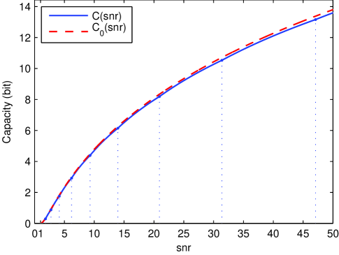
Figure 10: Capacity $C(\mathrm{snr})$ of heat channel, and its approximation $C_{0}(\mathrm{snr})$ in case $\alpha\beta=5$ (for larger values of $\alpha\beta$, the two curves quickly become indistinguishable in the given range of snr). Dotted lines depict snrs where differentiability of $C(\mathrm{snr})$ breaks down.

5.2.2 Discussion

To recognize the difference between Eqs. (46) and (49), we calculate the MMSE. We continue to suppose that $\mathrm{snr}=\sigma^{2}/\theta^{2}\geq 1$; the transpose of matrix $\boldsymbol{H}^{K}$ will be denoted by $\boldsymbol{H}^{KT}.$ Following [32], given

$$\boldsymbol{Y}^{K}=\sqrt{\mathrm{snr}}\boldsymbol{H}^{K}\boldsymbol{X}^{\prime K}+\boldsymbol{N}^{\prime K},$$ (51)

the MMSE in estimating $\boldsymbol{H}^{K}\boldsymbol{X}^{\prime K}$is

$$\mathrm{mmse}(\mathrm{snr}) = \mathbb{E}\left\|\boldsymbol{H}^{K}\boldsymbol{X}^{\prime K}-\boldsymbol{H}^{K}\widehat{\boldsymbol{X}^{\prime K}}\right\|^{2}$$

$$= \mathrm{tr}[\boldsymbol{H}^{K}(\boldsymbol{\Sigma}^{-K}+\mathrm{snr}{\boldsymbol{H}^{KT}}\boldsymbol{H}^{K})^{-1}{\boldsymbol{H}^{KT}}],$$

where $\widehat{\boldsymbol{X}^{\prime K}}$ is the minimum mean-square estimate of $\boldsymbol{X}^{\prime K}$, and $\boldsymbol{\Sigma}^{-K}$ is the inverse of the covariance matrix $\boldsymbol{\Sigma}^{K}$ of $\boldsymbol{X}^{\prime K}$. If $\boldsymbol{X}^{\prime K}$ has independent Gaussian components $X_{k}^{\prime}\sim\mathcal{N}(0,1-\mathrm{snr}^{-1}\rho^{-2k-1})$ as in Section 5.2.1, then $\boldsymbol{\Sigma}^{K}$ is a $K\times K$ diagonal matrix with entries $\sigma_{kk}=1-\mathrm{snr}^{-1}\rho^{-2k-1},\,k=0,\ldots,K-1$. A computation yields

$$\mathrm{mmse}(\mathrm{snr})=\sum_{k=0}^{K-1}\mathrm{snr}^{-1}\left(1-\mathrm{snr}^{-1}\rho^{-2k-1}\right).$$

When $\alpha\beta$ becomes large, we obtain by transition to a Riemann integral

$$\mathrm{mmse}(\mathrm{snr})\cdot\delta = \sum_{k=0}^{K-1}\mathrm{snr}^{-1}\left(1-\mathrm{snr}^{-1}\rho^{-2k-1}\right)\delta$$

$$= \mathrm{snr}^{-1}\int_{0}^{\infty}\left(1-\mathrm{snr}^{-1}e^{2x}\right)^{+}\,\mathrm{d}x+\epsilon$$

$$= \frac{1}{2}\frac{\ln\mathrm{snr}}{\mathrm{snr}}-\frac{1}{2}\frac{1}{\mathrm{snr}}\left(1-\frac{1}{\mathrm{snr}}\right)+\epsilon,$$

where $\epsilon\rightarrow 0$ as $\alpha\beta\rightarrow\infty$. Thus,

$$\mathrm{mmse}(\mathrm{snr})\doteq\frac{\alpha\beta}{2}\frac{\ln\mathrm{snr}}{\mathrm{snr}}-\frac{\alpha\beta}{2}\frac{1}{\mathrm{snr}}\left(1-\frac{1}{\mathrm{snr}}\right),$$

or, using Eq. (50),

$$\mathrm{mmse}(\mathrm{snr})\doteq\mathrm{node}(\mathrm{snr})-\frac{\alpha\beta}{2}\frac{1}{\mathrm{snr}}\left(1-\frac{1}{\mathrm{snr}}\right).$$ (52)

Finally, averaging with respect to the DOFs $\alpha\beta$ turns the (dotted) equations (50), (52) into true equations and we get for NODE and MMSE, resp.,

$$\overline{\mathrm{node}}(\mathrm{snr}) \triangleq\lim_{\alpha\beta\rightarrow\infty}\frac{\mathrm{node}(\mathrm{snr})}{\alpha\beta}=\frac{1}{2}\frac{\ln\mathrm{snr}}{\mathrm{snr}},$$

$$\overline{\mathrm{mmse}}(\mathrm{snr}) \triangleq\lim_{\alpha\beta\rightarrow\infty}\frac{\mathrm{mmse}(\mathrm{snr})}{\alpha\beta}=\overline{\mathrm{node}}(\mathrm{snr})-\frac{1}{2}\frac{1}{\mathrm{snr}}\left(1-\frac{1}{\mathrm{snr}}\right).$$

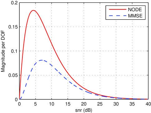
Figure 11: Magnitude per DOF of NODE and MMSE as DOFs $\alpha\beta\rightarrow\infty$.

In Fig. 11, $\overline{\mathrm{node}}(\mathrm{snr})$ and $\overline{\mathrm{mmse}}(\mathrm{snr})$ are plotted against $10\log_{10}\mathrm{snr}$ for $\mathrm{snr}\geq 1$. Apparently, the increase of capacity of the vector Gaussian channel (51) with growing snr as predicted by the C-NODE relationship of Th. 6 is significantly higher than anticipated by the I-MMSE relationship (46), at least in the lower snr region (and at the expense of higher dimension $K$ since $K\rightarrow\infty$ as $\alpha\beta\rightarrow\infty$). This observation might also be useful for the assessment of the capacity of (high dimensional) MIMO systems, where, by the way, the case of snr-dependent input signals has rarely been treated so far (cf., e.g., [32], [35], [36], [37]).

Appendix

Appendix A Wigner-Ville Spectrum of Filter Response on White Gaussian Noise

We model white Gaussian noise of two-sided noise PSD $\sigma^{2}\in(0,\infty)$ by a sequence of stochastic processes $\{\boldsymbol{U}^{K}(t),t\in\mathbb{R}\},\,K=1,2,\ldots,$ given by their respective Karhunen-Loève expansion

$$\boldsymbol{U}^{K}(t)=\sum_{k=0}^{K-1}U_{k}\,(D_{\gamma}\psi_{k})(t),\,t\in\mathbb{R},$$

where $U_{0},\ldots,U_{K-1}$ are $\mathrm{i.i.d.}$ Gaussian random variables $\sim\mathcal{N}(0,\sigma^{2})$. For any $K=1,2,\ldots,$ let the process $\{\boldsymbol{U}^{K}(t),t\in\mathbb{R}\}$ be the input to filter $\boldsymbol{P}_{\delta}^{(\gamma)}$. By means of representation (10) it is seen that the corresponding filter output tends as $K\rightarrow\infty$ to the stochastic process

$$X(t)=\sum_{k=0}^{\infty}\rho^{k+\frac{1}{2}}U_{k}\,(D_{\gamma}\psi_{k})(t),\,t\in\mathbb{R}.$$ (53)

We interprete $\{X(t),t\in\mathbb{R}\}$ as filter response on white Gaussian noise.

Since any realization $x(t)$ of $\{X(t)\}$ is almost surely in $L^{2}(\mathbb{R})$, the Wigner distribution [26]

$$(Wx)(t,\omega)=\frac{1}{2\pi}\int_{-\infty}^{\infty}e^{-i\omega t^{\prime}}x\left(t+\frac{t^{\prime}}{2}\right)\overline{x\left(t-\frac{t^{\prime}}{2}\right)}\,\mathrm{d}t^{\prime}$$

may be computed. By taking the ensemble average, we obtain the WVS [29] of process $\{X(t)\}$,

$$\boldsymbol{\Phi}(t,\omega) = \mathbb{E}[(WX)(t,\omega)]$$ (54)

$$= \frac{1}{2\pi}\int_{-\infty}^{\infty}e^{-i\omega t^{\prime}}r\left(t+\frac{t^{\prime}}{2},t-\frac{t^{\prime}}{2}\right)\,\mathrm{d}t^{\prime},$$

where $r(t_{1},t_{2})=\mathbb{E}[X(t_{1})\overline{X(t_{2})}]$ is the autocorrelation function. The kernel of operator $\boldsymbol{P}_{\delta}^{(\gamma)}$ has for arbitrary parameters $\gamma,\delta>0$ two alternative representations (following from a generalization of Mehler’s formula [16]),

$$P_{\delta}^{(\gamma)}(x,y)$$

$$=\sum_{k=0}^{\infty}\rho^{k+\frac{1}{2}}(D_{\gamma}\psi_{k})(x)(D_{\gamma}\psi_{k})(y)$$

$$=\frac{1}{\gamma\sqrt{2\pi\sinh\delta}}\exp\left\{-\frac{1}{4\gamma^{2}}\left[\coth\left(\frac{\delta}{2}\right)(x-y)^{2}+\tanh\left(\frac{\delta}{2}\right)(x+y)^{2}\right]\right\}.$$

We infer by the first representation that $r(t_{1},t_{2})=\sigma^{2}P_{2\delta}^{(\gamma)}(t_{1},t_{2})$. Then, by means of the second representation, the integral in (54) is readily evaluated; we obtain

$$\boldsymbol{\Phi}(t,\omega)=\frac{\sigma^{2}}{2\pi}\cdot\frac{1}{\cosh\delta}\exp\left(-\frac{t^{2}}{\alpha^{2}}-\frac{\omega^{2}}{\beta^{2}}\right).$$

Appendix B Proofs of Theorems 2 and 4

For a linear operator $A:L^{2}(\mathbb{R})\rightarrow L^{2}(\mathbb{R})$ the Weyl symbol $\sigma_{A}(x,\xi)$—when existing [26]—is defined by [27], [25]

$$(Af)(x)=\frac{1}{2\pi}\int\!\!\!\int_{\mathbb{R}^{2}}\sigma_{A}\left(\frac{x+y}{2},\xi\right)e^{i(x-y)\xi}f(y)\,\mathrm{d}y\,d\xi.$$ (55)

The linear map $A\mapsto\sigma_{A}(x,\xi)$ (or rather its inverse) is called Weyl correspondence. For example, the operator $A=\boldsymbol{P}_{2\delta}^{(\gamma)}$ has the Weyl symbol [16]

$$\sigma_{A}(x,\xi) = \frac{1}{\cosh\delta}e^{-(\tanh\delta)(\gamma^{-2}x^{2}+\gamma^{2}\xi^{2})}$$

$$= \frac{1}{\cosh\delta}\exp\left(-\frac{x^{2}}{\alpha^{2}}-\frac{\xi^{2}}{\beta^{2}}\right).$$

In the rest of this appendix, $A$ will always stand for operator $\boldsymbol{P}_{2\delta}^{(\gamma)}$, and $\lambda_{k},\,k=0,1,\ldots,$ for its eigenvalues $\rho^{2k+1}\in(0,1)$. The proof of the subsequent Th. 7 follows the argument in [25] (cf. also [23], [24]), although the Szegő theorems in [25], [24] are inadequate for our purposes.

Lemma 1.

For any polynomial $G_{N}(x,z)=\sum_{n=1}^{N}c_{n}(x)z^{n}$ with bounded variable coefficients $c_{n}(x)\in\mathbb{R}$, $x\in(1,\infty),$ it holds

$$\sum_{k=0}^{\infty}G_{N}(\alpha\beta,\lambda_{k})\doteq\frac{1}{2\pi}\int\!\!\!\int_{\mathbb{R}^{2}}G_{N}\left(\alpha\beta,\sigma_{A}(x,\xi)\right)\,\mathrm{d}x\,\mathrm{d}\xi.$$ (57)

Proof:.

First, by (10), for any $f\in L^{2}(\mathbb{R})$ it holds that

$$G_{N}(\alpha\beta,A)f=\sum_{k=0}^{\infty}G_{N}(\alpha\beta,\lambda_{k})\langle f,D_{\gamma}\psi_{k}\rangle D_{\gamma}\psi_{k}.$$

Hence, operator $B=G_{N}(\alpha\beta,A)$ has the trace

$$\mathrm{tr}\,B=\sum_{k=0}^{\infty}G_{N}(\alpha\beta,\lambda_{k}).$$ (58)

Second, we use the key observation [25, trace rule (0.4)] to obtain (here and thereafter, double integrals extend over $\mathbb{R}^{2}$)

$$\mathrm{tr}\,B=\frac{1}{2\pi}\int\!\!\!\int\sigma_{B}(x,\xi)\,\mathrm{d}x\,\mathrm{d}\xi,$$

where $\sigma_{B}(x,\xi)$ is the Weyl symbol of operator $B$. By linearity of the Weyl correspondence, $\sigma_{B}(x,\xi)$ has the expansion

$$\sigma_{B}(x,\xi)=\sum_{n=1}^{N}c_{n}(\alpha\beta)\sigma_{A^{n}}(x,\xi).$$

Since for any $\gamma>0$ held constant the family of operators $\{\boldsymbol{P}_{\delta}^{(\gamma)};\delta>0\}$ forms a semigroup with respect to $\delta$ (see [16]), it follows that $A^{n}=\boldsymbol{P}_{2n\delta}^{(\gamma)}$. In Eq. (B), replace operator $A$ by $A^{n}$ and $\delta$ by $n\delta$. Because of $\tanh(n\delta)=(n\tanh\delta)(1+o(1))$ we then obtain

$$\sigma_{A^{n}}(x,\xi) = \frac{1}{\cosh(n\delta)}e^{-\tanh(n\delta)(\gamma^{-2}x^{2}+\gamma^{2}\xi^{2})}$$

$$= (1+o(1))\left(\sigma_{A}(x,\xi)\right)^{n}\exp\left[-o(1)\left(\frac{x^{2}}{\alpha^{2}}+\frac{\xi^{2}}{\beta^{2}}\right)\right],$$

where the Landau symbol $o(1)$ stands for various quantities vanishing as $\delta\rightarrow 0$ (or $\alpha\beta\rightarrow\infty$). We now estimate

$$\mathrm{tr}\,B = \frac{1}{2\pi}\int\!\!\!\int\sigma_{B}(x,\xi)\,\mathrm{d}x\,\mathrm{d}\xi$$ (59)

$$= \left[\frac{1}{2\pi}\int\!\!\!\int G_{N}\left(\alpha\beta,\sigma_{A}(\alpha x,\beta\xi)\right)\,dx\,d\xi+\epsilon\right]\alpha\beta$$

$$= \frac{1}{2\pi}\int\!\!\!\int G_{N}(\alpha\beta,\sigma_{A}(x,\xi))\,\mathrm{d}x\,\mathrm{d}\xi+\epsilon\,\alpha\beta,$$

where $\epsilon\rightarrow 0$ as $\alpha\beta\rightarrow\infty$. Eq. (59) in combination with Eq. (58) concludes the proof. ∎

Theorem 7 (Szegő Theorem).

Let $g:[0,\Delta]\rightarrow\mathbb{R}$, $\Delta\in(0,\infty)$, be a continuous function such that $\lim_{x\rightarrow 0+}g(x)/x$ exists. For any functions $a,\,b:(1,\infty)\rightarrow\mathbb{R}$, where $a(x)$ is bounded and $b(x)\in[0,\Delta]$, define the function $G(x,z)=a(x)g(b(x)z),\,(x,z)\in(1,\infty)\times[0,1]$. Then it holds

$$\sum_{k=0}^{\infty}G(\alpha\beta,\lambda_{k})\doteq\frac{1}{2\pi}\int\!\!\!\int_{\mathbb{R}^{2}}G\left(\alpha\beta,\sigma_{A}(x,\xi)\right)\,\mathrm{d}x\,\mathrm{d}\xi.$$ (60)

Proof:.

The function $f(x)=g(x)/x,\,x\in(0,\Delta],$ has a continuous extension $F(x)$ onto the compact interval $[0,\Delta]$. By virtue of the Weiertstrass approximation theorem, for any $n\in\mathbb{N}$ there exists a polynomial $F_{N_{n}-1}(x)$ of some degree $N_{n}-1$ such that $|F(x)-F_{N_{n}-1}(x)|\leq\epsilon_{n}=\frac{1}{n}$ for all $x\in[0,\Delta]$. Consequently, the polynomial $g_{N_{n}}(x)=xF_{N_{n}-1}(x)$ of degree $N_{n}$ satisfies the inequality

$$|g(x)-g_{N_{n}}(x)|\leq\epsilon_{n}x,\,x\in[0,\Delta].$$ (61)

Define the polynomial with variable coefficients $G_{N_{n}}(x,z)=a(x)g_{N_{n}}(b(x)z)$. We now show that

$$(\alpha\beta)^{-1}\sum_{k=0}^{\infty}G_{N_{n}}(\alpha\beta,\lambda_{k})\rightarrow(\alpha\beta)^{-1}\sum_{k=0}^{\infty}G(\alpha\beta,\lambda_{k})$$ (62)

and

$$\frac{(\alpha\beta)^{-1}}{2\pi}\int\!\!\!\int_{\mathbb{R}^{2}}G_{N_{n}}\left(\alpha\beta,\sigma_{A}(x,\xi)\right)\,\mathrm{d}x\,\mathrm{d}\xi$$ (63)

$$\rightarrow \frac{(\alpha\beta)^{-1}}{2\pi}\int\!\!\!\int_{\mathbb{R}^{2}}G\left(\alpha\beta,\sigma_{A}(x,\xi)\right)\,\mathrm{d}x\,\mathrm{d}\xi,$$

as $n\rightarrow\infty$, uniformly for $\alpha\beta\in(1,\infty)$.

Proof of (62): By Ineq. (61) we get

$$|\sum_{k=0}^{\infty}G(\alpha\beta,\lambda_{k})-\sum_{k=0}^{\infty}G_{N_{n}}(\alpha\beta,\lambda_{k})| \leq \sum_{k=0}^{\infty}|G(\alpha\beta,\lambda_{k})-G_{N_{n}}(\alpha\beta,\lambda_{k})|$$

$$\leq M\epsilon_{n}\Delta\sum_{k=0}^{\infty}\lambda_{k},$$

where $M=\sup\{|a(x)|;x>1\}<\infty$ and $\sum_{k=0}^{\infty}\lambda_{k}=\rho/(1-\rho^{2})\leq\alpha\beta/2$ for $\alpha\beta>1$. After devision of the last inequality by $\alpha\beta$, convergence in (62) follows as claimed.

Proof of (63): Similarly,

$$|\int\!\!\!\int G\left(\alpha\beta,\sigma_{A}(x,\xi)\right)\,\mathrm{d}x\,\mathrm{d}\xi-\int\!\!\!\int G_{N_{n}}\left(\alpha\beta,\sigma_{A}(x,\xi)\right)\,\mathrm{d}x\,\mathrm{d}\xi|$$

$$\leq \int\!\!\!\int|G\left(\alpha\beta,\sigma_{A}(x,\xi)\right)-G_{N_{n}}\left(\alpha\beta,\sigma_{A}(x,\xi)\right)|\,\mathrm{d}x\,\mathrm{d}\xi$$

$$\leq M\epsilon_{n}\Delta\int\!\!\!\int\sigma_{A}(x,\xi)\,\mathrm{d}x\,\mathrm{d}\xi.$$

Since $(2\pi)^{-1}\int\!\!\!\int\sigma_{A}(x,\xi)\,\mathrm{d}x\,\mathrm{d}\xi=\rho/(1-\rho^{2})$, we arrive at the same conclusion as before.

Now, choose an arbitrarily large number $n\in\mathbb{N}$, substitute function $G$ in Eq. (60) by the polynomial $G_{N_{n}}$ and devide both sides of that equation by $\alpha\beta$. Then, by reason of Lem. 1 and uniform convergence in (62) and (63) with respect to $\alpha\beta\in(1,\infty)$, the theorem follows. ∎

Proof of Th. 2: Define

$$\ln_{+}x=\left\{\!\!\begin{array}[]{cl}\max\{0,\ln x\}&\mbox{if }x>0,\\ 0&\mbox{if }x=0.\end{array}\right.$$

Because of Eq. (19) we have, recalling that $\sigma^{2}$ is dependent on $\alpha\beta$,

$$C(S) = \sum_{k=0}^{\infty}\frac{1}{2}\ln_{+}\left(\frac{\sigma^{2}(\alpha\beta)}{\theta^{2}}\lambda_{k}\right)$$

$$= \sum_{k=0}^{\infty}a(\alpha\beta)g(b(\alpha\beta)\lambda_{k}),$$

where $a(\alpha\beta)=1$, $b(\alpha\beta)=\sigma^{2}(\alpha\beta)/\theta^{2}$, $g(x)=\frac{1}{2}\ln_{+}x,x\in[0,\Delta]$, and $\Delta$ is chosen so that $b(\alpha\beta)\leq\Delta<\infty$ when $\alpha\beta$ is large enough (the latter choice is possible since $\sigma^{2}(\alpha\beta)$ is finitely upper bounded as $\alpha\beta\rightarrow\infty$). Without loss of generality, we assume $b(\alpha\beta)\in[0,\Delta]$ for all $\alpha\beta\in(1,\infty)$. Then, by Th. 7 it follows that

$$C(S) \doteq \frac{1}{2\pi}\int\!\!\!\int_{\mathbb{R}^{2}}\frac{1}{2}\ln_{+}\left(\frac{\sigma^{2}(\alpha\beta)}{\theta^{2}}\sigma_{A}(x,\xi)\right)\,\mathrm{d}x\,\mathrm{d}\xi$$

$$= \frac{1}{2\pi}\int\!\!\!\int\frac{1}{2}\ln\left[1+\frac{\left(\frac{\sigma^{2}(\alpha\beta)}{2\pi}-N(x,\xi)\right)^{+}}{N(x,\xi)}\right]\,\mathrm{d}x\,\mathrm{d}\xi,$$

where $N(x,\xi)=\frac{\theta^{2}}{2\pi}(\sigma_{A}(x,\xi))^{-1}$. Next, rewrite Eq. (16) as

$$S=\sum_{k=0}^{\infty}\sigma^{2}(\alpha\beta)\left(1-\frac{1}{\frac{\sigma^{2}(\alpha\beta)}{\theta^{2}}\lambda_{k}}\right)^{+}.$$

Put $a(\alpha\beta)=\sigma^{2}(\alpha\beta)$, $b(\alpha\beta)=\sigma^{2}(\alpha\beta)/\theta^{2}$ and define

$$g(x)=\left\{\!\!\begin{array}[]{cl}\left(1-\frac{1}{x}\right)^{+}&\mbox{if }x>0,\\ 0&\mbox{if }x=0.\end{array}\right.$$

Without loss of generality, we assume that $a(\alpha\beta)$ is bounded for all $\alpha\beta\in(1,\infty)$. So, $b(\alpha\beta)\in[0,\Delta]$ where $\Delta=\sup\{a(\alpha\beta)/\theta^{2};\alpha\beta>1\}<\infty$. Then, by Th. 7 it follows that

$$S \doteq \frac{1}{2\pi}\int\!\!\!\int\sigma^{2}(\alpha\beta)\left(1-\frac{1}{\frac{\sigma^{2}(\alpha\beta)}{\theta^{2}}\sigma_{A}(x,\xi)}\right)^{+}\,\mathrm{d}x\,\mathrm{d}\xi$$

$$= \int\!\!\!\int\left(\frac{\sigma^{2}(\alpha\beta)}{2\pi}-N(x,\xi)\right)^{+}\,\mathrm{d}x\,\mathrm{d}\xi.$$

Finally, replacement of $\frac{\sigma^{2}(\alpha\beta)}{2\pi}$ by the parameter $\nu$ completes the proof. $\Box$

Proof of Th. 4: For any $\theta\in(0,\sigma]$ held constant define the distortion $D$ by Eq. (35) or, equivalently, by

$$D=\sum_{k=0}^{\infty}\theta^{2}\min\left\{1,\frac{\sigma^{2}}{\theta^{2}}\lambda_{k}\right\}.$$

Since $D=\sum_{k=0}^{\infty}a(\alpha\beta)g(b(\alpha\beta)\lambda_{k})$, where $a(\alpha\beta)=\theta^{2}$, $b(\alpha\beta)=\sigma^{2}/\theta^{2}$, $g(x)=\min\{1,x\}$ for $x\in[0,\Delta]$, $\Delta=\sigma^{2}/\theta^{2}$, it follows by Th. 7 that

$$D \doteq \frac{1}{2\pi}\int\!\!\!\int\theta^{2}\min\left\{1,\frac{\sigma^{2}}{\theta^{2}}\sigma_{A}(x,\xi)\right\}\,\mathrm{d}x\,\mathrm{d}\xi$$

$$= \int\!\!\!\int\min\left\{\frac{\theta^{2}}{2\pi},\boldsymbol{\Phi}(t,\omega)\right\}\,\mathrm{d}t\,\mathrm{d}\omega,$$

where $\boldsymbol{\Phi}(t,\omega)=\frac{\sigma^{2}}{2\pi}\,\sigma_{A}(t,\omega)$ is the WVS (14). Next, rewrite Eq. (38) as

$$R=\sum_{k=0}^{\infty}\frac{1}{2}\ln_{+}\left(\frac{\sigma^{2}}{\theta^{2}}\lambda_{k}\right).$$

Taking $a(\alpha\beta)=1$, $b(\alpha\beta)=\sigma^{2}/\theta^{2}$, $g(x)=\frac{1}{2}\ln_{+}x,x\in[0,\Delta]$, $\Delta$ chosen as before, we infer by Th. 7 that

$$R \doteq \frac{1}{2\pi}\int\!\!\!\int_{\mathbb{R}^{2}}\frac{1}{2}\ln_{+}\left(\frac{\sigma^{2}}{\theta^{2}}\sigma_{A}(x,\xi)\right)\,\mathrm{d}x\,\mathrm{d}\xi$$

$$= \frac{1}{2\pi}\int\!\!\!\int\frac{1}{2}\ln_{+}\left[\frac{\boldsymbol{\Phi}(t,\omega)}{\frac{\theta^{2}}{2\pi}}\right]\,\mathrm{d}t\,\mathrm{d}\omega.$$

Finally, replacement of $\frac{\theta^{2}}{2\pi}$ by the parameter $\lambda$ completes the proof. $\Box$

References

- [1] E. Hammerich, “On the heat channel and its capacity,” Proc. IEEE Int. Symp. Information Theory, Seoul, Korea, 2009, pp. 1809–1813.
- [2] J. Fourier, The Analytical Theory of Heat. Mineola, NY: Dover Publ., 2003. (engl. transl. of Fourier’s 1822 book)
- [3] A. N. Tikhonov, V. Y. Arsenin, and F. John (Transl.), Solutions of ill-posed problems, Washington, DC: Winston, 1977.
- [4] D. D. Falconer, “History of equalization 1860–1980,” IEEE Commun. Mag., vol. 49, pp. 42–50, 2011.
- [5] G. P. Agrawal, Fiber-optic communication systems. 3rd ed. New York, NY: Wiley, 2002.
- [6] R.-J. Essiambre, G. Kramer, P. J. Winzer, G. J. Foschini, and B. Goebel, “Capacity limits of optical fiber networks,” J. Lightw. Technol., vol. 28, pp. 662–701, 2010.
- [7] P. J. Winzer and R.-J. Essiambre, “Advanced optical modulation formats,” in Optical Fiber Telecommunications V B, I. P. Kaminov, T. Li, and A. E. Willner, Eds. San Diego, CA: Academic Press, pp. 23–94, 2008.
- [8] R. G. Gallager, Information Theory and Reliable Communication. New York: Wiley, 1968.
- [9] S. M. Moser, “Capacity results of an optical intensity channel with input-dependent Gaussian noise,” IEEE Trans. Inf. Theory, vol. 58, pp. 207–223, 2012.
- [10] C. E. Shannon, “A mathematical theory of communication,” Bell Syst. Tech. J., vol. 27, pt. I, pp. 379–423, 1948; pt. II, pp. 623–656, 1948.
- [11] T. M. Cover and J. A. Thomas, Elements of Information Theory. 2nd ed. Hoboken, NJ: Wiley, 2006.
- [12] I. Daubechies, Ten Lectures on Wavelets. Philadelphia, PA: SIAM, 1992.
- [13] I. Daubechies, “Time-frequency localization operators: A geometric phase space approach,” IEEE Trans. Inf. Theory, vol. 34, pp. 605–612, 1988.
- [14] H. Cramér, Mathematical Methods of Statistics. Princeton, NJ: Princeton Univ. Press, 1946.
- [15] H. Gross, Handbook of Optical Systems, Vol. 1. Weinheim: Wiley-VCH, 2005.
- [16] E. Hammerich, “A sampling theorem for time-frequency localized signals,” Sampl. Theory Signal Image Process., vol. 3, pp. 45–81, 2004.
- [17] D. Gabor, “Theory of communication,” J. Inst. Elect. Eng. (London), vol. 93 (III), pp. 429–457, 1946.
- [18] E. Getzler, “A short proof of the local Atiyah-Singer index theorem,” Topology, vol. 25, pp. 111–117, 1985.
- [19] D. O. North, Analysis of the factors which determine signal/noise discrimination in pulsed-carrier systems. Rept. PTR-6C, RCA Labs., Princeton, NJ, 1943.
- [20] G. L. Turin, “An introduction to matched filters,” IRE Trans. Inf. Theory, vol. 6, pp. 311–329, 1960.
- [21] M. Abramowitz and I. A. Stegun, Handbook of Mathematical Functions. New York, NY: Dover Publ., 1972.
- [22] R. M. Corless, G. H. Gonnet, D. E. G. Hare, D. J. Jeffrey, and D. E. Knuth, “On the Lambert function,” Adv. Computational Math., vol. 5, pp. 329–359, 1996.
- [23] P. Jung, “On the Szegö-asymptotics for doubly-dispersive Gaussian channels,” Proc. IEEE Int. Symp. Information Theory, St. Petersburg, Russia, 2011, pp. 2852–2856.
- [24] H. G. Feichtinger and K. Nowak, “A Szegö-type theorem for Gabor-Toeplitz localization operators,” Michigan Math. J., vol. 49, pp. 13–21, 2001.
- [25] A. J. E. M. Janssen and S. Zelditch, “Szegö limit theorems for the harmonic oscillator,” Trans. Amer. Math. Soc., vol. 280, pp. 563–587, 1983.
- [26] K. Gröchenig, Foundations of Time-Frequency Analysis. Boston: Birkhäuser, 2001.
- [27] W. Kozek and F. Hlawatsch, “Time-frequency representation of linear time-varying systems using the Weyl symbol,” in Proc. IEE Sixth Int. Conf. on Digital Signal Process. in Commun., Loughborough, UK, pp. 25–30, 1991.
- [28] F. Hlawatsch and W. Kozek, “Second-order time-frequency synthesis of nonstationary random processes,” IEEE Trans. Inf. Theory, vol. 41, pp. 255–267, 1995.
- [29] P. Flandrin and W. Martin, “The Wigner-Ville spectrum of nonstationary random signals,” in The Wigner Distribution, W. Mecklenbräuker and F. Hlawatsch, Eds. Amsterdam: Elsevier, 1997, pp. 211–267.
- [30] A. N. Kolmogorov, “On the Shannon theory of information transmission in the case of continuous signals,” IRE Trans. Inf. Theory, vol. 2, pp. 102–108, 1956.
- [31] T. Berger, Rate Distortion Theory: A Mathematical Basis for Data Compression. Englewood Cliffs, NJ: Prentice-Hall, 1971.
- [32] D. Guo, S. Shamai (Shitz), and S. Verdú, “Mutual information and minimum mean-square error in Gaussian channels,” IEEE Trans. Inf. Theory, vol. 51, pp. 1261–1282, 2005.
- [33] C. E. Shannon, “Communication in the presence of noise,” Proc. IRE, vol. 37, pp. 10–21, 1949.
- [34] E. Hammerich, “Correction to ‘A note on Gallager’s capacity theorem for waveform channels’,” 2013 [Online]. Available: arXiv:1207.4707v2
- [35] İ. E. Telatar, “Capacity of multi-antenna Gaussian channels,” Europ. Trans. Telecommun., vol. 10, pp. 585–595, 1999.
- [36] A. L. Lozano, A. M. Tulino, and S. Verdú, “Optimum power allocation for parallel Gaussian channels with arbitrary input distributions,” IEEE Trans. Inf. Theory, vol. 52, pp. 3033–3051, 2006.
- [37] D. Palomar and S. Verdú, “Representation of mutual information via input estimates,” IEEE Trans. Inf. Theory, vol. 53, pp. 453–470, 2007.