Exact Tkachenko modes and their damping in the vortex lattice regime of rapidly rotating bosons

Abstract

We have found an exact analytical solution of the Bogoliubov-de Gennes equations for the Tkachenko modes of the vortex lattice in the lowest Landau level (LLL) in the thermodynamic limit at any momenta and calculated their damping rates. At finite temperatures both Beliaev and Landau damping leads to momentum independent damping rates in the low-energy limit, which shows that at sufficiently low energies Tkachenko modes become strongly damped. We then found that the mean square fluctuations of the density grow logarithmically at large distances, which indicates that the state is ordered in the vortex lattice only on a finite (although exponentially large) distance scale and introduces a low-momentum cut-off. Using this circumstance we showed that at finite temperatures the one-body density matrix undergoes an exponential decay at large distances.

I Introduction

The physics of rapidly rotating Bose-condensed gases is governed by a collective behavior of nucleated vortices (see Zwerger ; coop ; revfet for review). When the rotation frequency $\Omega$ along the axis perpendicular to the plane of rotation $(x,y)$ is close to the trapping frequency $\omega$ in the $x$ and $y$ directions, the harmonically trapped Bose gas becomes essentially two-dimensional (2D) and can be described as a system of interacting bosons in the lowest Landau level (LLL). If the number of vortices is much smaller than the number of particles, the system is in the so-called ”mean-field” quantum Hall regime ho , where vortices arrange themselves in a lattice with an intervortex spacing of the order of the ”magnetic length” $l=\hbar/\sqrt{m\Omega}$. Under an increase in $\Omega$ the vortex lattice should melt and strongly correlated Quantum Hall states should emerge.

The vortex lattice in the LLL or close to this regime has been obtained experimentally exp1 ; exp2 ; exp3 and studied theoretically assuming the presence of a macroscopic wave function $\Psi(\bf{r})$ (see revfet for review and refs. in us ). Presently, a new generation of experiments with rapidly rotating quantum gases is being set up. It is based on the use of artificial gauge potentials, which are obtained by means of combinations of laser fields and mimic the rotation of the system (see Zwerger for review). They are supposed to provide the ”rotation” with frequency that is extremely close to $\omega$, thus allowing for the observation of the lattice melting and for the emergence of strongly correlated states. This puts forward the question of correlation properties in the vortex lattice regime and revives the interest to excitation modes in this regime.

The theory of elastic oscillations of a vortex lattice in incompressible superfluids has been constructed by Tkachenko tk , and a linear spectrum of the wave dispersion has been obtained. The effect of a finite compressibility has been discussed in Refs. vol-doz ; son ; baym1 , and it has been shown that the compressibility changes dramatically the dispersion relation in the low-momentum limit. The dispersion becomes quadratic due to hybridization with sound waves. The first experimental observation of Tkachenko modes in harmonically trapped Bose-condensed gases has been reported in Ref.exp1 . Theoretical analysis of these modes has been done in the mean-field approach for both the geometry of an infinite plane ($\Omega=\omega$) and in the presence of remaining trapping anglin ; baym2 ; baym3 ; sonin1 ; sonin2 ; mizushima ; baksmaty ; cozzini . The calculations provided an explanation of the mode frequencies observed in the experiment exp1 . Theoretical studies based on the microscopic effective action showed the absence of long-range order at $T=0$ in the thermodynamic limit (infinite plane geometry) sinova , and the hydrodynamic approach revealed an algebraic decay of the one-body density matrix at large distances baym3 .

In this paper we find an exact analytical solution of the Bogoliubov-de Gennes equations for the Tkachenko modes of the LLL vortex lattice in the thermodynamic limit at any momenta and calculate their damping rates. Importantly, at finite temperatures both Beliaev and Landau damping mechanisms lead to momentum independent damping rates in the low-energy limit. This means that for sufficiently low energies the Tkachenko modes become strongly damped, which is consistent with the experimental results exp1 . Using the obtained results for the excitation wavefunctions we then calculate the mean square fluctuations of the density and the one-body denity matrix. The density fluctuations grow logarithmically at large distances, which indicates that the state is ordered in the vortex lattice only on a finite (although exponentially large) distance scale and introduces a low-momentum cut-off. Using this circumstance we show that at finite temperatures the one-body density matrix undergoes an exponential decay at large distances.

II The ground state and equations for the excitations in the LLL approximation.

We consider a zero-temperature two-dimensional (2D) system of bosonic atoms in a harmonic trapping potential $V(r)=m\omega^{2}r^{2}/2$, rotating with frequency $\Omega$ around the axis perpendicular to the $(x,y)$ plane. In the rotating frame the Hamiltonian has the form:

$$H=\int d^{2}{\bf{r}}\,\left[\hat{\psi}^{\dagger}\frac{\hat{{\bf p}}^{2}}{2m}\hat{\psi}+\frac{g}{2}\hat{\psi}^{\dagger}\hat{\psi}^{\dagger}\hat{\psi}\hat{\psi}+V({\bf r})\hat{\psi}^{\dagger}\hat{\psi}-\Omega\hat{\psi}^{\dagger}\hat{L}_{z}\hat{\psi}\right],$$ (1)

where $\hat{\psi}({\bf{r}})$ is the field operator, $\hat{{\bf p}}$ is the momentum operator, $m$ is the atom mass, $\hat{L}_{z}$ is the operator of the orbital angular momentum, and $g$ is the coupling constant for short-range atom-atom interaction. The non-linear Schroedinger equation for $\hat{\psi}({\bf r},t)$ reads:

$$i\hbar\frac{\partial\hat{\psi}}{\partial t}=\frac{\hat{{\bf p}}^{2}}{2m}\hat{\psi}+g\hat{\psi}^{\dagger}\hat{\psi}\hat{\psi}+V({\bf r})\hat{\psi}-\Omega\hat{L}_{z}\hat{\psi}.$$ (2)

It is commonly assumed that in the mean-field Quantum Hall regime all particles are in the same macroscopic quantum state described by the wavefunction $\Psi$. Zwerger ; coop ; revfet ; ho . In the ground state this wavefunction has the form $\Psi({\bf r},t)=\Psi_{0}({\bf r})\exp(-i\mu t)$, where $\mu$ is the chemical potential. The wavefunction $\Psi_{0}({\bf r})$ is then governed by the Gross-Pitaevskii equation:

$$\frac{\hat{{\bf p}}^{2}}{2m}\Psi_{0}+g|\Psi_{0}|^{2}\Psi_{0}+V({\bf r})\Psi_{0}-\Omega\hat{L}_{z}\Psi_{0}=\mu\Psi_{0},$$ (3)

where it is normalized to the total number of particles $N$. For $\Omega$ close to $\omega$, the ground state of the system corresponds to the LLL and, hence, the macroscopic wave function $\Psi_{0}(\bf{r})$ takes the form:

$$\Psi_{0}({\bf{r}})=\sqrt{n}f_{0}(z)\mbox{e}^{-|z|^{2}/2},$$ (4)

where $n=N/S$ is the mean density, with $S$ being the surface area, $z,\bar{z}=(x\pm iy)/l$, and the function $f_{0}(z)$ is analytical in the $(x,y)$ plane, with $f_{0}(z)\exp(-|z|^{2}/2)$ normalized to unity. Equation (3) is then solved numerically by expressing $\Psi_{0}$ as a superposition of the LLL single-particle eigenfunctions $z^{n}\exp(-|z|^{2}/2)/\sqrt{\pi n!}$. Alternatively, one solves a projected Gross-Pitaevskii equation obtained by acting on Eq. (3) with the LLL projection operator $\hat{P}$. This operator acts on an arbitrary function $F(z,\bar{z})$ as

$$\hat{P}F(z,\bar{z})=\frac{1}{\pi}\int dwd\bar{w}\exp[-|w|^{2}+z\bar{w}]F(w,\bar{w}),$$ (5)

and transformes it to the function in the LLL.

For $\Omega=\omega$ we have the geometry of an infinite plane. The LLL is infinitely degenerate and the projected Gross-Pitaevskii equation reads

$$\frac{Ng}{\pi}\int dwd\bar{w}\mbox{e}^{-2w\bar{w}+z\bar{w}}|f_{0}(w)|^{2}f_{0}(w)=\tilde{\mu}f_{0}(z),$$ (6)

where $\tilde{\mu}=\mu-\hbar\Omega$.

The ground state solution of Eq. (6) is a triangular vortex lattice and the function $f_{0}(z)$ is expressed through the Jacobi Theta-function $\vartheta_{1}$ us :

$$f_{0}(z)=(2v)^{1/4}\vartheta_{1}(\sqrt{\pi v}z,q)\,\mbox{e}^{z^{2}/2},$$ (7)

with $q=\exp(i\pi\tau)$, $\tau=u+iv$, $v=\sqrt{3}/2$, $u=-1/2$. The chemical potential is then equal to $\tilde{\mu}=\alpha ng$, with $\alpha=\sqrt{v}\sum_{m,p}(-1)^{mp}\exp\{-\pi v(m^{2}+p^{2})\}=1.1596$.

An alternative mean-field approach does not apriori assume the presence of long-range order and is based on the density-phase formalism. It is commonly employed for 2D Bose-condensed gases at finite temperatures and for weakly interacting 1D bosons, where the long-range order is destroyed by long-wave fluctuations of the phase. The key condition of this approach is related to small fluctuations of the density. One writes the field operator in the form

$$\hat{\psi}=\exp i\hat{\Phi}\,\sqrt{\hat{n}};\,\,\,\,\,\,\,\hat{\psi}^{\dagger}=\sqrt{\hat{n}}\exp{(-i\hat{\Phi})}$$ (8)

with $\hat{n}$ and $\hat{\Phi}$ being the density and phase operators satisfying the the commutation relation $[\hat{n}({\bf r}),\hat{\phi}({\bf r}^{\prime})]=i\delta({\bf r}-{\bf r}^{\prime})$. Representing these operators as $n=n_{0}({\bf{r}})+\delta\hat{n}$ and $\Phi=\Phi_{0}({\bf{r}})+\delta\hat{\Phi}$, one writes Eq. (2) in terms of the density and phase keeping only zero and first order terms in small fluctuations $\delta\hat{n}$ and $\nabla\delta\hat{\Phi}$. To zero order we then have Eq. (2) for $\Psi_{0}({\bf r})=\sqrt{n_{0}({\bf r})}\exp(i\Phi_{0}({\bf r}))$ and, hence, the projected equation (5) for the function $f_{0}(z)$ introduced by Eq. (4). The solutions of two equations that are linear in $\delta\hat{n}$ and $\nabla\delta\hat{\Phi}$ are obtained by representing these quantities in terms of elementary excitations characterized by the wavenumber ${\bf k}=\{k_{x},k_{y}\}$:

$$\delta\hat{n}=\sqrt{n_{0}}\mbox{e}^{-|z|^{2}/2}\sum_{{\bf k}}[u_{{\bf k}}\exp[-i\Phi_{0}]-\tilde{v}^{*}_{{\bf k}}\exp[i\Phi_{0}]]\exp[-i\epsilon_{{\bf k}}t]\hat{a}_{{\bf k}}+h.c.$$ (9)

$$\delta\hat{\Phi}=\frac{-i\mbox{e}^{-|z|^{2}/2}}{2\sqrt{n_{0}}}\sum_{{\bf k}}[u_{{\bf k}}\exp[-i\Phi_{0}]+\tilde{v}^{*}_{{\bf k}}\exp[i\Phi_{0}]]\exp[-i\epsilon_{{\bf k}}t]\hat{a}_{{\bf k}}+h.c.,$$ (10)

where $\hat{a}_{{\bf k}}$, $\hat{a}_{{\bf k}}^{\dagger}$ are operators of anihilation/creation of the excitations, and the functions $u_{{\bf k}},\tilde{v}_{{\bf k}}$ satisfy the Bogoliubov-de Gennes equations. In the LLL approximation they are analytical functions of $z$ and follow from the projected Bogoliubov-de Gennes equations:

$$2g\hat{P}(|\Psi_{0}|^{2}u_{{\bf k}})-g\hat{P}(\Psi_{0}^{2}\tilde{v}^{*}_{{\bf k}}) = (\tilde{\mu}+\epsilon_{{\bf k}})u_{{\bf k}}$$

$$2g\hat{P}(|\Psi_{0}|^{2}\tilde{v}_{{\bf k}})-g\hat{P}(\Psi_{0}^{2}{u}^{*}_{{\bf k}}) = (\tilde{\mu}-\epsilon_{{\bf k}})\tilde{v}_{{\bf k}}.$$ (11)

III Exact solution of the projected Bogoliubov-de Gennes equations

In this section we will use coordinates expressed in units of $l$, wavevectors in units of $l^{-1}$, and energies in units of $ng$. The exact solution of Eqs. (11) for the functions $u_{{\bf k}},\,\tilde{v}_{{\bf k}}$ reads:

$$u_{{\bf k}}=\frac{c_{1{\bf k}}}{\sqrt{S}}f_{0}\left(z+\frac{ik_{+}}{2}\right)\mbox{e}^{ik_{-}z/2}\mbox{e}^{-k^{2}/4}=c_{1{\bf k}}P(f_{0}\mbox{e}^{i\bf{kr}})$$ (12)

$$\tilde{v}_{{\bf k}}=\frac{c_{2{\bf k}}}{\sqrt{S}}f_{0}\left(z-\frac{ik_{+}}{2}\right)\mbox{e}^{-ik_{-}z/2}\mbox{e}^{-k^{2}/4}=c_{2{\bf k}}P(f_{0}\mbox{e}^{-i\bf{kr}}),$$ (13)

where $k_{\pm}=k_{x}\pm ik_{y}$, and the coefficients $c_{1{\bf k}},\,c_{2{\bf k}}$ follow from the normalization condition $\int dx\,dy(|u_{{\bf k}}|^{2}-|v_{{\bf k}}^{2})\mbox{e}^{-|z|^{2}}=1$. They are given by

$$c_{1{\bf k}}=\left[\frac{\tilde{K}({\bf k})+\epsilon_{{\bf k}}}{2\epsilon_{{\bf k}}}\right]^{1/2}\mbox{e}^{k^{2}/8},$$ (14)

$$c_{2{\bf k}}=\left[\frac{\tilde{K}({\bf k})-\epsilon_{{\bf k}}}{2\epsilon_{{\bf k}}}\right]^{1/2}\frac{|K_{2}({\bf k})|}{K_{2}({\bf k})}\mbox{e}^{k^{2}/8},$$ (15)

with

$$\tilde{K}({\bf k})=2K_{1}({\bf k})-K_{1}(0),$$ (16)

$$K_{1}({\bf{k}})=\sqrt{v}\sum_{n,m=-\infty}^{\infty}(-1)^{nm}\mbox{e}^{-\pi v(n^{2}+m^{2})}\mbox{e}^{-\sqrt{\pi v}k_{x}n+i\sqrt{\pi v}k_{y}m}\mbox{e}^{-k_{x}^{2}/4},$$ (17)

$$K_{2}({\bf{k}})=\sqrt{v}\sum_{n,m=-\infty}^{\infty}(-1)^{nm}\mbox{e}^{-\pi v(n^{2}+m^{2})}\mbox{e}^{-\sqrt{\pi v}(k_{x}-ik_{y})(n+m)}\mbox{e}^{-k_{x}^{2}/2+ik_{x}k_{y}/2},$$ (18)

and

$$K_{1}(0)=K_{2}(0)=\tilde{K}(0)=\alpha\simeq 1.1596.$$ (19)

The sums in Eqs. (17) and (18) can be expressed in terms of Jacobi Theta-functions:

$$K_{1}({\bf{k}})=\frac{e^{-\frac{{k_{y}}^{2}}{4}}\left(\vartheta_{3}\left(\frac{{k_{x}}\sqrt{\pi}}{2\sqrt{v}},e^{-\frac{\pi}{v}}\right)\vartheta_{3}\left(-\frac{i{k_{y}}\sqrt{\pi}}{4\sqrt{v}},e^{-\frac{\pi}{4v}}\right)+\vartheta_{2}\left(\frac{{k_{x}}\sqrt{\pi}}{2\sqrt{v}},e^{-\frac{\pi}{v}}\right)\vartheta_{4}\left(-\frac{i{k_{y}}\sqrt{\pi}}{4\sqrt{v}},e^{-\frac{\pi}{4v}}\right)\right)}{2v}$$ (20)

$$\begin{split}K_{2}({\bf{k}})=\frac{1}{2v}e^{-\frac{1}{2}{k_{y}}({k_{y}}+i{k_{x}})}\bigg{[}\vartheta_{3}\left(\frac{({k_{x}}-i{k_{y}})\sqrt{\pi}}{2\sqrt{v}},e^{-\frac{\pi}{v}}\right)\vartheta_{3}\left(\frac{({k_{x}}-i{k_{y}})\sqrt{\pi}}{4\sqrt{v}},e^{-\frac{\pi}{4v}}\right)\\ +\vartheta_{2}\left(\frac{({k_{x}}-i{k_{y}})\sqrt{\pi}}{2\sqrt{v}},e^{-\frac{\pi}{v}}\right)\vartheta_{4}\left(\frac{({k_{x}}-i{k_{y}})\sqrt{\pi}}{4\sqrt{v}},e^{-\frac{\pi}{4v}}\right)\bigg{]}\end{split}$$

The spectrum of excitations has the form (see Fig. 1 and Fig. 2):

$$\epsilon_{{\bf k}}^{2}=|2K_{1}({\bf{k}})-K_{0}|^{2}-|K_{2}({\bf{k}})|^{2},$$ (21)

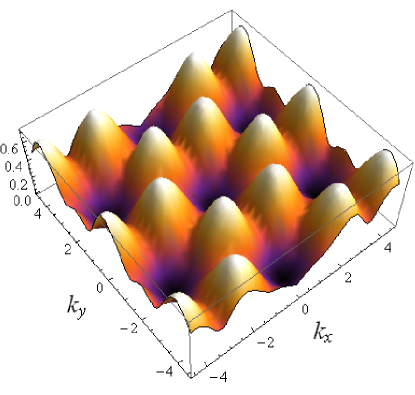
Figure 1: Excitation energy $\epsilon(k_{x},k_{y})$ in units of $ng$.

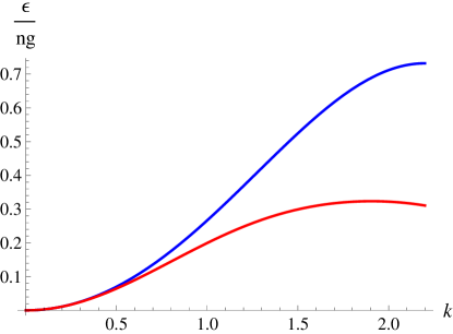
Figure 2: Anisotropy of the dispersion relation (21). The upper curve is $\epsilon(k,0)$, the lower curve is $\epsilon(k\cos\frac{\pi}{6},k\sin\frac{\pi}{6})$, and the directions $x$ and $y$ are chosen in the same way as in Fig. 1.

It is consistent with the spectrum obtained in the hydrodynamic approach baym2 ; baym3 ; sonin2 , but we clearly identify the anisotropy: for a given $k$ the excitation energy is maximal in the $x$ direction, and minimal at an angle of 30 degrees from the $x$ axis. (see Fig. 2). In the limit of small $k$, using the expansion of the functions $K_{1}({\bf k})$ and $K_{2}({\bf k})$:

$$K_{1}=\alpha\left[1-\frac{k^{2}}{8}+\frac{(\eta+1)k^{4}}{64}\right];\quad K_{2}=\alpha\left(1-\frac{k^{2}}{4}+\frac{k^{4}}{32}\right),$$ (22)

where

$$\eta=-8\,\frac{\sum_{m,p}(-1)^{mp}m^{2}p^{2}\exp[-\pi v(m^{2}+p^{2})]}{\sum_{m,p}(-1)^{mp}\exp[-\pi v(m^{2}+p^{2})]}\simeq 0.8219,$$

we find a symmetric spectrum. Restoring the dimensions it reads:

$$\epsilon=\frac{\alpha\sqrt{\eta}}{4}\,ng(kl)^{2}\simeq 0.2628\,ng\,(kl)^{2},$$ (23)

which exactly coincides with the hydrodynamic result of Ref. sonin2 . The obtained excitations are commonly termed as Tkachenko modes, although they have a quite different dispersion relation compared to elastic oscillations of the vortex lattice in incompressible superfluids obtained by Tkachenko tk .

For atoms (tightly) confined to the quasi2D geometry with frequency $\omega_{0}$, the coupling constant for the interatomic interaction is $g=2\sqrt{2\pi}\hbar^{2}a/ml_{0}$, where $a$ is the 3D scattering length, and $l_{0}=\sqrt{\hbar/m\omega_{0}}$. In the case of ⁸⁷Rb rotating in the $(x,y)$ plane with frequency $\Omega\simeq 100$ Hz and confined in the perpendicular direction with $\omega_{0}\simeq 300$ Hz, one has $ng/\hbar\Omega\simeq 0.1$ at the 2D density $n\simeq 3\times 10^{8}$ cm^-2, which justifies the LLL approximation. Then, low-energy excitations have frequencies below 1 Hz. Note that for this example the quantity $\nu=\pi nl^{2}$ representing the ratio of the number of particles to the number of vortices, i.e. the filling factor, is large and we are well in the mean-field regime.

IV Damping rates of the excitations

Let us now calculate the damping of these excitations, which is caused by the interaction term of the Hamiltonian (1), containing a product of four field operators. For finding the damping rate it is sufficient to use a linearized form of the field operator, i.e. put $\hat{\psi}=\Psi_{0}(1+\delta\hat{n}/2n_{0}+i\delta\hat{\Phi})$. Using equations (4), (9) and (10) we then have:

$$\hat{\psi}=\left(\sqrt{n}f_{0}(z)+\sum_{{\bf k}}[u_{{\bf k}}\hat{a}_{{\bf k}}\exp(-i\epsilon_{{\bf k}}t)-\tilde{v}_{{\bf k}}\hat{a}^{\dagger}_{{\bf k}}\exp(i\epsilon_{{\bf k}}t)\right)\exp(-i\mu t-|z|^{2}/2).$$ (24)

We first consider the Beliaev damping mechanism LL9 in which a given excitation with wavevector ${\bf p}$ decays into two excitations with lower energies and wavevectors (${\bf k}$ and ${\bf q}$). The part of the interaction Hamiltonian that causes the Beliaev damping contains three operators of the excitations and has the form:

$$\hat{V}=g\sqrt{n}\sum_{{\bf k},{\bf q}}\int dx\,dy\left[f_{0}u_{{\bf p}}u_{{\bf k}}^{*}u_{{\bf q}}^{*}+2f_{0}\tilde{v}_{{\bf p}}^{*}u_{{\bf q}}^{*}\tilde{v}_{{\bf k}}-f_{0}^{*}\tilde{v}_{{\bf p}}^{*}\tilde{v}_{{\bf k}}\tilde{v}_{{\bf q}}-2f_{0}^{*}u_{{\bf p}}u_{{\bf k}}^{*}\tilde{v}_{{\bf q}}\right]\mbox{e}^{-2|z|^{2}}\hat{a}_{{\bf q}}^{\dagger}\hat{a}_{{\bf k}}^{\dagger}\hat{a}_{{\bf p}}\,+h.c.$$ (25)

At a finite temperature $T$ we have to take into account thermal occupation of the states with momenta ${\bf k}$ and ${\bf q}$ and the presence of the reversed process in which excitations with momenta ${\bf k}$ and ${\bf q}$ recombine into the excitation with momentum ${\bf p}$. Using the Fermi golden rule the damping rate is given by

$$\Gamma_{{\bf p}}=\frac{2\pi}{\hbar}\sum_{{\bf k},{\bf q}}|\langle{\bf k},{\bf q}|\hat{V}|{\bf p}\rangle|^{2}(1+N_{{\bf k}}+N_{{\bf q}})\delta(\epsilon_{{\bf p}}-\epsilon_{{\bf k}}-\epsilon_{{\bf q}}),$$ (26)

with $N_{{\bf k},{\bf q}}=[\exp(\epsilon_{{\bf k},{\bf q}}/T)-1]^{-1}$ being equilibrium occupation numbers for the excitations. The excitation energy thus acquires the imaginary part and becomes $\epsilon_{{\bf p}}-i\hbar\Gamma_{{\bf p}}/2$.

For performing the calculations it is convenient to use the functions $u_{{\bf k}},\,v_{{\bf k}}$ in the form of Bloch waves:

$$u_{{\bf k}}({\bf r})\exp(-|z|^{2}/2)=c_{1{\bf k}}\frac{\Psi_{0}(z+ik_{+}l/2)}{\sqrt{N}}\exp(-k^{2}l^{2}/8)\exp(i{\bf k}{\bf r}/2),$$ (27)

$$v_{{\bf k}}({\bf r})\exp(-|z|^{2}/2)=c_{2{\bf k}}\frac{\Psi_{0}(z-ik_{+}l/2)}{\sqrt{N}}\exp(-k^{2}l^{2}/8)\exp(-i{\bf k}{\bf r}/2).$$ (28)

In the low-energy limit where $pl\ll 1$, the transition matrix element is equal to

$$\langle{\bf k},{\bf q}|\hat{V}|{\bf p}\rangle=\frac{\alpha^{5/2}}{S}\sqrt{\frac{Nng}{8\epsilon_{p}\epsilon_{k}\epsilon_{q}}}\,\left\{\frac{\epsilon_{k}}{\tilde{K}(k)}+\frac{\epsilon_{q}}{\tilde{K}(q)}-\frac{\epsilon_{p}}{\tilde{K}(p)}\right\}\,\delta_{{\bf p},{\bf k}+{\bf q}},$$ (29)

where $\delta_{{\bf p},{\bf k}+{\bf q}}$ is the Kronecker symbol. After a straightforward algebra Eq. (29) is reduced to

$$\langle{\bf k},{\bf q}|\hat{V}|{\bf p}\rangle=\frac{\alpha}{4\sqrt{2}\,\eta^{1/4}}\sqrt{\frac{ng^{2}}{S}}\,\frac{(k^{4}+q^{4}-p^{4})l}{kqp}\,\delta_{{\bf p},{\bf k}+{\bf q}}.$$ (30)

Equation (26) then yields:

$$\Gamma_{p}=\frac{\alpha^{2}}{8\sqrt{\eta}}\frac{ng^{2}l^{2}}{\hbar}\int_{0}^{p}kdk\int_{0}^{2\pi}\frac{d\phi}{2\pi}\,\frac{k^{2}(p^{2}-k^{2})}{p^{2}}\coth\left(\frac{\epsilon_{k}}{T}\right)\delta\left[\frac{\alpha\sqrt{\eta}}{4}ngl^{2}(p^{2}-k^{2}-(p^{2}+k^{2}-2kp\cos\phi)\right],$$

and we obtain:

$$\Gamma_{p}=\frac{\alpha}{8\pi\eta}\,\frac{g}{\hbar}\,p^{2}\int_{0}^{1}dxx^{2}\sqrt{1-x^{2}}\,\coth\left(\frac{\epsilon_{p}}{2T}\,x^{2}\right).$$ (31)

At $T=0$ we immediately find:

$$\Gamma_{p0}=\frac{\alpha}{128\eta}\,\frac{g}{\hbar}\,p^{2}\simeq 0.011\frac{g}{\hbar}\,p^{2}.$$ (32)

For the ratio of the damping rate to the excitation energy we then obtain:

$$\frac{\hbar\Gamma_{p0}}{\epsilon_{p}}=\simeq\frac{0.13}{\nu}.$$ (33)

In the mean-field regime we should have $\nu=\pi nl^{2}\gg 1$, since this quantity (filling factor) represents the ratio of the number of particles to the number of vortices. Therefore, we have $\hbar\Gamma_{p0}\ll\epsilon_{p}$ at any $p$. Thus, at $T=0$ Tkachenko modes are good elementary excitations in the entire mean-field Quantum Hall regime.

The situation changes drastically at finite temperatures. Equation (31) yields $\Gamma_{p0}+\Gamma_{pT}$, and for $\epsilon_{p}\ll T$ the temperature-dependent part of the damping rate is independent of $p$ and proves to be

$$\Gamma_{pT}=\frac{\pi}{4\eta^{3/2}}\,\frac{T}{\hbar}\,\frac{1}{\nu}\simeq 1.05\frac{T}{\hbar}\,\frac{1}{\nu};\,\,\,\,\,\,\epsilon_{p}\ll T.$$ (34)

For excitation energies $\epsilon_{p}\gg T/\nu$ we have $\hbar\Gamma_{pT}\ll\epsilon_{p}$, i.e. the damping rate is small and, hence, Tkachenko modes are good elementary excitations. Moreover, for $\epsilon_{p}>T$ the damping rate starts to decrease with increasing $p$. In particular, for $\epsilon_{p}\gg T$ equation (31) gives:

$$\Gamma_{pT}=\frac{\sqrt{\pi}}{4\eta^{3/2}}\,\zeta(3/2)\frac{T}{\hbar\nu}\left(\frac{T}{\epsilon_{p}}\right);\,\,\,\,\,\epsilon_{p}\gg T,$$ (35)

where $\zeta(3/2)$ is the Riemann zeta-function, and the imaginary part of the excitation energy is negligible compared to the real part $\epsilon_{p}$. However, excitations with energies

$$\epsilon_{p}\lesssim\epsilon_{c}=\frac{T}{\nu}$$ (36)

are overdamped.

Note that our analysis was assuming the so-called collisionless regime, where pumping the mode with a given energy $\epsilon_{p}$ one does not disturb the equilibrium distribution function $N_{k}$ for thermal excitations involved in the damping process. This means that the relaxation of their distribution function occurs on a time scale $\tau_{R}\gg\hbar/\epsilon_{p}$. For the discussed Beliaev damping, the thermal excitations that are involved in the damping of the mode with energy $\epsilon_{p}$ also have energies $\sim\epsilon_{p}$. So, we have $\tau_{R}\sim\Gamma_{p}^{-1}$, and excitations with energies $\epsilon_{p}\gg\epsilon_{c}$ are well in the collisionless regime. However, for $\epsilon_{p}\lesssim\epsilon_{c}$ we have the condition $\tau_{R}\epsilon_{p}/\hbar\lesssim 1$, and these excitations enter the hydrodynamic regime (see PS ). A dimensional estimate for their damping rate is $\Gamma\sim\Gamma_{p}(\epsilon_{p}\tau_{R}/\hbar)$, with $\Gamma_{p}$ being the damping rate in the collisionless regime. Thus, for the modes with energies $\epsilon_{p}\lesssim\epsilon_{c}$ we have the damping rate approaching $\epsilon_{p}$, i.e. they are significantly damped.

It should be noted that at finite temperatures we also have the Landau damping in which a given excitation with momentum ${\bf p}$ interacts with a thermal excitation (momentum ${\bf k}$), both are annihilated and an excitation with a higher energy and momentum (${\bf q}$) is created. There is a reversed process as well. The interaction Hamiltonian that causes this damping is:

$$\hat{V}_{L}=g\sqrt{n}\sum_{{\bf k},{\bf q}}\int dxdy\left[f_{0}^{*}u_{{\bf q}}^{*}u_{{\bf k}}u_{{\bf p}}+2f_{0}^{*}\tilde{v}_{{\bf k}}^{*}\tilde{v}_{{\bf q}}u_{{\bf p}}-f_{0}\tilde{v}_{{\bf k}}^{*}\tilde{v}_{{\bf p}}^{*}\tilde{v}_{{\bf q}}-2f_{0}u_{{\bf q}}^{*}\tilde{v}_{{\bf p}}^{*}u_{{\bf k}}\right]\,+h.c.,$$

and for the damping rate we have

$$\Gamma_{pL}=\frac{2\pi}{\hbar}\sum_{{\bf k},{\bf q}}|\langle{\bf q}|\hat{V}_{L}|{\bf p},{\bf k}\rangle|^{2}(N_{k}-N_{q})\delta(\epsilon_{q}-\epsilon_{p}-\epsilon_{k}).$$

The calculations are similar to those made above for the Beliaev damping. In the low-energy limit in both limiting cases, $\epsilon_{p}\ll T$ and $\epsilon_{p}\gg T$, the results are the same as in the case of Beliaev damping, but with a twice as small numerical coefficient. Thermal excitations that are involved in the damping of the mode with energy $\epsilon_{p}$ also have energies $\sim\epsilon_{p}$. We thus see that the Landau damping does not change our conclusion made from the analysis of the Beliaev damping. Namely, excitations with energies $\epsilon_{p}\gg\epsilon_{c}$ are well in the collisionless regime, with the damping rate $\Gamma_{p}\ll\epsilon/\hbar$. On the other hand, excitations with energies $\epsilon_{p}\lesssim\epsilon_{c}$ enter the hydrodynamic regime and are significantly damped.

For temperatures of the order of tens of nanokelvins and filling factors $\nu$ of the order of hundreds, like in experiments exp2 ; exp3 where the LLL regime has been reached, Tkachenko modes with frequencies of the order of 1 Hz or lower should already be in the regime of strong damping. The strong damping of Tkachenko modes in this frequency range has been observed in the JILA experiment exp1 , although this experiment was not yet in the LLL regime.

V One-body density matrix

We now discuss correlation properties of rapidly rotating bosons in the mean-field Quantum Hall regime at zero and finite temperatures. For this purpose we will use the field operators in the form (8). Due to small fluctuations of the density the one-body density matrix takes the form:

$$g_{1}({\bf r})=\langle\hat{\psi}^{\dagger}({\bf r})\hat{\psi}(0)\rangle=\Psi_{0}^{*}({\bf r})\Psi_{0}(0)\exp\left\{-\frac{1}{2}\langle(\delta\hat{\Phi}({\bf r})-\delta\hat{\Phi}(0))^{2}\rangle\right\}.$$ (37)

In the low-momentum limit where $kl\ll 1$, omitting the term $ik_{+}l/2$ in the argument of $\Psi_{0}$ in equations (27) and (28), the operator of the phase fluctuations given by Eq. (10) becomes:

$$\delta\hat{\Phi}({\bf r})=-\frac{i}{2}\sum_{{\bf k}}\frac{(c_{1{\bf k}}+c_{2{\bf k}})}{\sqrt{N}}\exp(i{\bf k}{\bf r}/2)\,\hat{a}_{{\bf k}}\,+h.c.$$ (38)

Then, using equations (14) and (15) for the mean square fluctuations we obtain:

$$\langle(\delta\hat{\Phi}({\bf r})-\delta\hat{\Phi}(0))^{2}\rangle=\alpha g\int\frac{d^{2}k}{(2\pi)^{2}}\,\frac{(1+2N_{k})}{\epsilon_{k}}[1-J_{0}(kr/2)],$$ (39)

where $J_{0}$ is the Bessel function.

At $T=0$ using the low-energy spectrum (23) equation (39) immediately gives:

$$\langle(\delta\hat{\Phi}({\bf r})-\delta\hat{\Phi}(0))^{2}\rangle_{0}=\frac{2}{\sqrt{\eta}}\,\frac{1}{\nu}\int_{0}^{p_{0}}\frac{dk}{k}\,[1-J_{0}(kr/2)].$$ (40)

The upper bound of the integration in Eq. (41) is $p_{0}\sim 1/l$, which represents the boundary of the first Brilluen zone, and for $r\gg l$ we find

$$\langle(\delta\hat{\Phi}({\bf r})-\delta\hat{\Phi}(0))^{2}\rangle_{0}\simeq\frac{2}{\sqrt{\eta}}\,\frac{1}{\nu}\ln\left(\frac{e^{C}r}{2l}\right),$$ (41)

with $C=0.5772$ being the Euler constant. For the density matrix we then have an algebraic decay at large distances:

$$g_{1}(r)\propto\left(\frac{l}{r}\right)^{1/\sqrt{\eta}\pi nl^{2}},\,\,\,\,\,\,\,\,r\gg l,$$ (42)

which reproduces the result of Ref. baym3 . So, in the thermodynamic limit there is no long-range order even at $T=0$, and we are dealing with a phase-fluctuating Bose-condensed state.

At finite temperatures we have to take into account thermal fluctuations of the phase. Before finding $g_{1}({\bf r})$ we calculate the mean square fluctuations of the density $\langle(\delta\hat{n}({\bf r})-\delta\hat{n}(0))^{2}\rangle/n^{2}$, which should be small for the validly of the mean-field approach. This is the case at $T=0$, but at finite temperatures thermal fluctuations drastically change the situation. Using equations (9), (27), and (28) in the low-momentum limit we have:

$$\frac{\langle(\delta\hat{n}({\bf r})-\delta\hat{n}(0))^{2}\rangle}{n^{2}}=\int_{0<k<l^{-1}}\frac{d^{2}k}{(2\pi)^{2}}\,\frac{g\alpha k^{2}l^{2}}{2\epsilon_{k}}[1-J_{0}(kr/2)](1+2N_{k}).$$ (43)

For obtaining this relation we put $c_{1k}=c_{2k}=\alpha$ and expanded $\Psi_{0}(z+ik+l/2)$ in powers of $k$ up to the first order. Then, omitting small vacuum fluctuations and writing $N_{k}\simeq T/\epsilon_{k}$ we reduce Eq. (43) to

$$\frac{\langle(\delta\hat{n}({\bf r})-\delta\hat{n}(0))^{2}\rangle}{n^{2}}=\frac{4T}{\alpha\eta ng\nu}\int_{0}^{\tilde{l}^{-1}}[1-J_{0}(kr/2)]\frac{dk}{k},$$ (44)

where $\tilde{l}=l$ for $T\gg ng$, and for $T\ll ng$ we have $\tilde{l}=k_{T}^{-1}$ with the momentum $k_{T}$ following from the condition $\epsilon_{k_{T}}=T$. The integration is straightforward and it yields:

$$\frac{\langle(\delta\hat{n}({\bf r})-\delta\hat{n}(0))^{2}\rangle}{n^{2}}\simeq\frac{4T}{\alpha\eta ng\nu}\ln\left(\frac{r}{2\tilde{l}}\right),$$ (45)

i.e. the density fluctuations grow logarithmically with the distance. This means that at finite temperatures the mean-field approach can be employed only on a distance scale $r<r_{0}=2\tilde{l}\exp(\alpha\eta ng\nu/4T)$. Then the mean square fluctuations of the density are small. In other words, the state is ordered in the vortex lattice only at $r<r_{0}$.

This introduces a low-momentum cut-off $r_{0}^{-1}$. For the thermal mean square fluctuations of the phase we then have:

$$\langle(\delta\hat{\Phi}({\bf r})-\delta\hat{\Phi}(0))^{2}\rangle=\frac{2\alpha g}{\pi}\int_{r_{0}^{-1}}^{l^{-1}}\frac{kdk}{\epsilon_{k}}\,\frac{[1-J_{0}(kr/2)]}{\exp(\epsilon_{k}/T)-1}.$$ (46)

The most important contribution to the integral comes from low momenta, so that we can expand the exponent in the denominator of Eq. (46) and put the upper limit of integration equal to infinity. Then Eq. (46) takes the form:

$$\langle(\delta\hat{\Phi}({\bf r})-\delta\hat{\Phi}(0))^{2}\rangle=\frac{32T}{\alpha\eta ng\nu}\int_{r_{0}^{-1}}^{\infty}\frac{dk}{k^{3}}[1-J_{0}(kr/2)],$$ (47)

A straightforward integration at distances $r\gg l$ yields:

$$\langle(\delta\hat{\Phi}({\bf r})-\delta\hat{\Phi}(0))^{2}\rangle=\frac{8T}{\alpha\eta ng\nu}\frac{r^{2}}{l^{2}}\ln\left(\frac{r_{0}}{r}\right).$$ (48)

Omitting vacuum phase fluctuations we then obtain an exponential decay of the density matrix:

$$g_{1}(r)\propto\exp\left[-\frac{4T}{\alpha\eta ng\nu}\frac{r^{2}}{l^{2}}\ln\left(\frac{r_{0}(T)}{r}\right)\right].$$ (49)

For systems with a finite size $L<r_{0}$ we have to replace $r_{0}$ with $L$ in Eq. (49).

Stricktly speaking, equation (49) is applicable only at distances $r\ll r_{0}$, where the system is ordered in the lattice. However, we clearly see that for $r$ approaching $r_{0}$ the density matrix practically drops to zero and, hence, it should remain close to zero at larger distances.

VI Concluding remarks

Concluding our work we would like to make a few remarks. First of all, the length scale $r_{0}$ on which the system is ordered in the vortex lattice at finite temperatures is exponentially large and in cold atom experiments it exceeds the size of the sample. Even on approach to the melting point, assuming $T\simeq ng$ and $\nu\simeq 20$ we have $r_{0}\simeq 300l$. However, the effect of finite temperature is likely to be dramatic for the visibility of the vortices. Equation (45) shows that even fairly well in the mean-field regime, for example at $\nu\simeq 40$ the mean square fluctuations of the density are $\langle(\delta\hat{n}({\bf r})-\delta\hat{n}(0))^{2}\rangle\sim 0.3$ for $r\simeq 10l$ and $T\simeq ng$. This should significantly reduce the visibility of the vortices. We do not claim that these arguments explain the reduction of the vortex visibility in the ENS experiment exp3 , but rather attract attention to this finite-temperature effect for future studies.

It is also worth mentioning that at finite temperatures the damping of Tkachenko modes may serve as a signature of the approach to the melting point of the lattice. The characteristic excitation energy $\epsilon_{c}\simeq T/\nu$ below which these modes are strongly damped, increases significantly with decreasing the filling factor and becomes of the order of $10$ Hz for $\nu=40$ even at temperatures as low as 20 nK.

References

• (1) I. Bloch, J. Dalibard, and W. Zwerger, Rev. Mod. Phys. 80, 885 (2008).
• (2) N. R. Cooper, Advances in Physics 57, 539 (2008).
• (3) A. L. Fetter, Rev. Mod. Phys. 81, 647 (2009).
• (4) Tin-Lun Ho, Phys. Rev. Lett. 87, 060403 (2001).
• (5) I. Coddington, P. Engels,V. Schweikhard, and E. A. Cornell, Phys. Rev. Lett. 91, 100402 (2003).
• (6) V. Schweikhard, I. Coddington, P. Engels, V. P. Mogendorff, and E. A. Cornell, Phys. Rev. Lett. 92, 040404 (2004).
• (7) V. Bretin, S. Stock, Y. Seurin, and J. Dalibard, Phys. Rev. Lett. 92, 050403 (2004).
• (8) S. I. Matveenko, D. Kovrizhin, S. Ouvry, and G. V. Shlyapnikov, Phys. Rev. A 80, 063621 (2009); S. I. Matveenko, Phys. Rev. A 82, 033628 (2010).
• (9) V. K. Tkachenko, Zh. Eksp. Teor. Fiz. 50, 1573 (1966) [Sov. Phys. JETP 23, 1049 (1966)].
• (10) G. Baym and E. Chandler, J. Low Temp. Phys. 50, 57 (1983); 62, 119 (1986).
• (11) G.E. Volovik and V.S. Dotsenko (jr), Pisma Zh. Eksp. Teor. Fiz. 29, 630 (1979) [JETP Lett. 29, 576 (1979)].
• (12) E. B. Sonin, Rev. Mod. Phys. 59, 87 (1987).
• (13) J.R. Anglin and M. Crescimanno, cond-mat/0210063.
• (14) G. Baym, Phys. Rev. Lett. 91, 110402 (2003).
• (15) G. Baym, Phys. Rev. A 69, 043618 (2004).
• (16) T. Mizushima, Y. Kawaguchi, K. Machida, T. Ohmi, T. Isoshima, and M. Salomaa, Phys. Rev. Lett. 92, 060407 (2004).
• (17) L.O. Baksmaty, S.J. Woo, S. Choi, and N.P. Bigelow, Phys. Rev. Lett. 92, 160405 (2004).
• (18) E.B. Sonin, Phys. Rev. A 71, 011603(R) (2005).
• (19) E. B. Sonin, Phys. Rev. A 72, 021606(R) 2005.
• (20) M. Cozzini, L. P. Pitaevskii, and S. Stringari, Phys. Rev. Lett. 92, 220401 (2004).
• (21) J. Sinova, C. B. Hanna, and A. H. MacDonald, Phys. Rev. Lett. 89, 030403 (2002).
• (22) E.M. Lifshitz and L.P. Pitaevskii, Statistical Physics Part 2 (Pergamon Press, Oxford, 1980).
• (23) L. P. Pitaevskii and S. Stringari, Bose-Einstein Condensation (Oxford University Press, Oxford, 2003).