Numerical Study of breakup in generalized Korteweg-de Vries and Kawahara equations

Abstract

This article is concerned with a conjecture in [8] on the formation of dispersive shocks in a class of Hamiltonian dispersive regularizations of the quasilinear transport equation. The regularizations are characterized by two arbitrary functions of one variable, where the condition of integrability implies that one of these functions must not vanish.

It is shown numerically for a large class of equations that the local behaviour of their solution near the point of gradient catastrophe for the transport equation is described locally by a special solution of a Painlevé-type equation. This local description holds also for solutions to equations where blow up can occur in finite time.

Furthermore, it is shown that a solution of the dispersive equations away from the point of gradient catastrophe is approximated by a solution of the transport equation with the same initial data, modulo terms of order $\epsilon^{2}$ where $\epsilon^{2}$ is the small dispersion parameter. Corrections up to order $\epsilon^{4}$ are obtained and tested numerically.

1 Introduction

Many wave phenomena in dispersive media with negligible dissipation, in hydrodynamics, nonlinear optics, and plasma physics are described by nonlinear dispersive partial differential equations (PDE). These equations are also mathematically challenging since the solutions can have highly oscillatory regions and blowup even for smooth initial data (see, e.g., [28], [16], [17]).

This article is concerned with a conjecture in [8] on the formation of dispersive shocks [16], [23], [26] in a class of Hamiltonian regularizations of the quasilinear transport equation

$$u_{t}+a(u)u_{x}=0,\quad a^{\prime}(u)\neq 0,\quad u,x\in\mathbb{R}.$$ (1.1)

In the present paper we will consider general Hamiltonian perturbations of (1.1) up to fourth order in a small dispersion parameter $0<\epsilon\ll 1$. They can be written in the form of a conservation law

$$u_{t}+a(u)u_{x}+\epsilon^{2}\partial_{x}\left\{b_{1}(u)u_{xx}+b_{2}(u)u_{x}^{2}+\epsilon\left[b_{3}(u)u_{xxx}+b_{4}(u)u_{xx}u_{x}+b_{5}(u)u_{x}^{3}\right]\right.$$

$$\left.+\epsilon^{2}\left[b_{6}(u)u_{xxxx}+b_{7}(u)u_{xxx}u_{x}+b_{8}(u)u_{xx}^{2}+b_{9}(u)u_{xx}u_{x}^{2}+b_{10}(u)u_{x}^{4}\right]\right\}=0,$$ (1.2)

where the coefficients $b_{1}(u)$, …, $b_{10}(u)$ are smooth functions satisfying certain constraints following from the existence of a Hamiltonian representation

$$u_{t}+\partial_{x}\frac{\delta H}{\delta u(x)}=0,$$

(see Corollary 2.2 below). Here and below we use the notation

$$\partial_{x}=\frac{\partial}{\partial x}.$$

This class of equations contains important equations as the Korteweg-de Vries (KdV) equation $u_{t}+6uu_{x}+\epsilon^{2}u_{xxx}=0$ and its generalizations, the Kawahara equation and the Camassa-Holm equation in an asymptotic sense (see [8]).

Up to certain equivalencies the Hamiltonian regularizations of (1.1) are characterized by two free functions $c(u)$ and $p(u)$:

$$u_{t}+a(u)u_{x}+{\epsilon^{2}}\partial_{x}\left[c\,a^{\prime}u_{xx}+\frac{1}{2}(c\,a^{\prime})^{\prime}u_{x}^{2}\right]+\epsilon^{4}\partial_{x}\left[\left(2p\,a^{\prime}+\frac{3}{5}{c^{2}a^{\prime\prime}}\right)u_{xxxx}+\dots\right]=0.$$ (1.3)

Two equations of the form (1.3) with the same invariants $c(u)$ and $p(u)$ commute, up to order ${\mathcal{O}}(\epsilon^{6})$

$$\left(u_{t}\right)_{\tilde{t}}-\left(u_{\tilde{t}}\right)_{t}={\mathcal{O}}\left(\epsilon^{6}\right)$$

where, for an arbitrary function $\tilde{a}=\tilde{a}(u)$

$$u_{\tilde{t}}+\tilde{a}(u)u_{x}+{\epsilon^{2}}\partial_{x}\left[c\,\tilde{a}^{\prime}u_{xx}+\frac{1}{2}(c\,\tilde{a}^{\prime})^{\prime}u_{x}^{2}\right]+\epsilon^{4}\partial_{x}\left[\left(2p\,\tilde{a}^{\prime}+\frac{3}{5}{c^{2}\tilde{a}^{\prime\prime}}\right)u_{xxxx}+\dots\right]=0.$$

In this paper the analysis of [8] up to order $\epsilon^{4}$ is extended to higher orders of $\epsilon$. Our analysis suggests that the only obstruction to the functions $c(u)$ and $p(u)$ by the condition of integrability is the condition that $c(u)$ must not vanish.

We then proceed to the study of the critical behaviour of solutions to (1). Namely, let $(x_{c},t_{c},u_{c})$ be a point of gradient catastrophe of a solution $u^{0}(x,t)$ to (1.1) specified by an initial value $u^{0}(x,0)=\phi(x)$. This means that the solution is a smooth function of $(x,t)$ for sufficiently small $|x-x_{c}|$ and $t-t_{c}<0$. Moreover there exists the limit

$$\lim_{x\to x_{c},\,t\to t_{c}-0}u^{0}(x,t)=u_{c},$$

but the derivatives $u_{x}^{0}(x,t)$, $u_{t}^{0}(x,t)$ blow up at the point. The Universality Conjecture of [8] says that, up to shifts, Galilean transformations and rescalings, the behavior at the point of gradient catastrophe of a solution to (1) with the same $\epsilon$-independent initial data $\phi(x)$ essentially depends neither on the choice of the generic solution nor on the choice of the generic equation. Moreover, the generic solution near this point $(x_{c},t_{c},u_{c})$ is given by

$$u(x,t,\epsilon)\simeq u_{c}+\alpha\,\epsilon^{2/7}U\left(\dfrac{x-x_{c}-a_{0}(t-t_{c})}{\beta\,\epsilon^{6/7}};\dfrac{t-t_{c}}{\gamma\,\epsilon^{4/7}}\right)+O\left(\epsilon^{4/7}\right),$$ (1.4)

where $a_{0}=a(u_{c})$ and the constants $\alpha$, $\beta$, $\gamma$ depend on the choice of the generic equation and the solution

$$\alpha=\left(\frac{12b_{1}^{0}}{a_{0}^{\prime}k^{2}}\right)^{1/7},$$

$$\beta=\left(\frac{12^{3}k\,(b_{1}^{0})^{3}}{{a_{0}^{\prime}}^{3}}\right)^{1/7},$$ (1.5)

$$\gamma=\left(\frac{12^{2}k^{3}(b_{1}^{0})^{2}}{{a_{0}^{\prime}}^{9}}\right)^{1/7}.$$

Here $a_{0}^{\prime}=a^{\prime}(u_{c})$, $b_{1}^{0}=b_{1}(u_{c})$; it is assumed that $b_{1}^{0}\neq 0$. The constant $k$ in these formula is inverse proportional to the “strength” of the breakup of the dispersionless solution $u^{0}(x,t)$

$$k=-6\lim_{x\to x_{c}}\frac{x-x_{c}}{\left(u^{0}(x,t_{c})-u_{c}\right)^{3}}$$ (1.6)

where we assume that $k\neq 0$ (another genericity hypothesis) and $a_{0}^{\prime}k>0$.

The function $U=U(X;T)$, $(X,T)\in\mathbb{R}^{2}$, is defined as the unique real smooth solution to the fourth order ODE [1], [19]

$$X=T\,U-\left[\frac{1}{6}U^{3}+\frac{1}{24}U_{X}^{2}+\frac{1}{12}U\,U_{XX}+\frac{1}{240}U_{XXXX}\right],$$ (1.7)

which is the second member of the Painlevé I hierarchy. We will call this equation PI2.

The relevant solution is characterized by the asymptotic behavior

$$U(X,T)=-(6X)^{\frac{1}{3}}-\dfrac{2^{2/3}T}{(3X)^{\frac{1}{3}}}+O(X^{-\frac{5}{3}}),\quad X\to\pm\infty,$$ (1.8)

for each fixed $T\in\mathbb{R}$. The existence of a smooth solution of (1.7) for all real $X,T$ satisfying (1.8) has been proved by Claeys and Vanlessen [5].

Observe that the principal term of the asymptotics (1.4) depends only on the order $\epsilon^{2}$ regularization. In the present paper we will numerically analyze, in particular, the influence of the higher order corrections on the local behaviour of solutions to (1) near the point of catastrophe.

First numerical tests of the PI2 asymptotic description of the critical point for the class of PDE in [8] have been presented in [15] for the KdV and the Camassa-Holm equation. In [4] a rigourous proof of the asymptotic behaviour (1.4) has been obtained for the KdV equation.

In this paper we generalize the numerical investigation of [15] to a larger class of equations which include the generalized KdV equation, the Kawahara equations with a dispersion of fifth order and the second equation in the KdV hierarchy.

We comment on the formation of blow up and on the role of integrability in the formation of oscillatory regions. In particular we show the differences in the formation of dispersive shock waves between integrable and non-integrable cases. The KdV equation has been extensively studied numerically in [14].

Then we show numerically that the solution of the dispersive equation (1) converges to the solution of the dispersionless equation (1.1) away from the point of gradient catastrophe at a rate of order $\epsilon^{2}$. Finally we show that the solution of the dispersive equation (1) is well approximated as a series in even power of $\epsilon$ in terms of the solution of the dispersionless equation (1.1) up to order $\epsilon^{4}$ by the so called quasi-triviality transformation [8] away from the point of gradient catastrophe. Such an approximation has already been obtained for conservation laws with positive viscosity [13]. Furthermore the existence of an expansion in even powers of $\epsilon$ has already appeared and been proved in the context of large $N$ expansions in Hermitian matrix models [3],[12].

The paper is organized as follows. In sect. 2 we briefly review the results of [8]. In sect. 3 we discuss higher order in $\epsilon$ regularizations of (1.1) and obstructions on the function $c(u)$ by the condition of integrability. A numerical study of the applicability of the conjecture to generalized KdV equations is given in sect. 4. We also comment on the possibility of blowup. In sect. 5 the conjecture is tested numerically for equations with high order dispersion as the Kawahara equation. Differences in the formation of rapid oscillations in the solutions to integrable and non-integrable equations are studied. Details about the used numerical methods are given in the appendix.

2 Hamiltonian PDEs and their invariants

In this paper we mainly study scalar Hamiltonian PDEs of the order at most five. They are written in the form of a conservation law

$$u_{t}+\partial_{x}\varphi(u,\epsilon\,u_{x},\epsilon^{2}u_{xx},\epsilon^{3}u_{xxx},\epsilon^{4}u_{xxxx})=0,$$ (2.9)

where

$$\varphi=\frac{\delta H}{\delta u(x)},$$

$$H=\int h(u,\epsilon\,u_{x},\epsilon^{2}u_{xx})\,dx.$$

Recall that the Euler–Lagrange derivative is defined by

$$\frac{\delta H}{\delta u(x)}=\frac{\partial h}{\partial u}-\partial_{x}\frac{\partial h}{\partial u_{x}}+\partial_{x}^{2}\frac{\partial h}{\partial u_{xx}}-\dots.$$ (2.11)

Here and in the sequel the integral of a differential polynomial is understood, in the spirit of formal calculus of variations, as the equivalence class of the polynomial modulo the image of the operator of total $x$-derivative

$$\partial_{x}h=u_{x}\frac{\partial h}{\partial u}+u_{xx}\frac{\partial h}{\partial u_{x}}+\dots.$$ (2.12)

It is worthwhile to recall that a differential polynomial $p(u;u_{x},\dots,u^{(m)})$ belongs to ${\rm Im}\,\partial_{x}$ iff

$$\frac{\delta P}{\delta u(x)}=0,\quad P=\int p(u;u_{x},\dots,u^{(m)})\,dx.$$ (2.13)

The Poisson bracket of two local functionals $H$, $F$ associated with (2.9), (2), is a local functional of the form

$$\{H,F\}=\int\frac{\delta H}{\delta u(x)}\frac{d}{dx}\frac{\delta F}{\delta u(x)}\,dx$$ (2.14)

Lemma 2.1.

Equation (2.9) can be written in the Hamiltonian form (2) iff the function $\varphi$ satisfies the following two constraints

$$\frac{\partial\varphi}{\partial u_{x}}=\partial_{x}\left[\frac{\partial\varphi}{\partial u_{xx}}-\frac{1}{2}\partial_{x}\frac{\partial\varphi}{\partial u_{xxx}}\right]$$

(2.15)

$$\frac{\partial\varphi}{\partial u_{xxx}}=2\partial_{x}\frac{\partial\varphi}{\partial u_{xxxx}}.$$

Proof  According to the classical Helmholtz criterion (see in [7]) the function $\varphi(u,u_{x},u_{xx},\dots)$ can be locally represented as the variational derivative of some functional $H=\int h(u,u_{x},\dots)\,dx$ iff it satisfies the following system of constraints

$$\frac{\partial\varphi}{\partial u^{(i)}}=(-1)^{i}\sum_{m\geq 0}\frac{(m+i)!}{i!~{}m!}(-\partial_{x})^{m}\frac{\partial\varphi}{\partial u^{(i+m)}},\quad i=0,\,1,\,\dots.$$ (2.16)

For the particular case under consideration the equations (2.16) reduce to (2.1).    

Applying the Lemma to a PDE (2.9) written in the form of the weak dispersion expansion one arrives at

Corollary 2.2.

The equation

$$u_{t}+a(u)u_{x}+\partial_{x}\left\{\epsilon\,b_{0}(u)u_{x}+\epsilon^{2}\left[b_{1}(u)u_{xx}+b_{2}(u)u_{x}^{2}\right]+\epsilon^{3}\left[b_{3}(u)u_{xxx}+b_{4}(u)u_{xx}u_{x}+b_{5}(u)u_{x}^{3}\right]\right.$$

$$\left.+\epsilon^{4}\left[b_{6}(u)u_{xxxx}+b_{7}(u)u_{xxx}u_{x}+b_{8}(u)u_{xx}^{2}+b_{9}(u)u_{xx}u_{x}^{2}+b_{10}(u)u_{x}^{4}\right]\right\}=0$$ (2.17)

is Hamiltonian iff the coefficients $b_{0}$, …, $b_{10}$ satisfy

$$b_{0}=0,$$

$$b_{2}=\frac{1}{2}b_{1}^{\prime},$$

$$b_{3}=0,$$

$$b_{5}=\frac{1}{3}b_{4}^{\prime},$$

$$b_{7}=2b_{6}^{\prime},$$

$$b_{8}=\frac{3}{2}b_{6}^{\prime},$$

$$b_{10}=\frac{1}{4}b_{9}^{\prime}.$$

The Hamiltonian equations (2.9) are considered modulo canonical transformations written in the form of a time-$\epsilon$ shift

$$u(x)\mapsto\tilde{u}(x)=u(x)+\epsilon\{u(x),K\}+\frac{\epsilon^{2}}{2!}\left\{\{u(x),K\},K\right\}+\dots$$ (2.18)

generated by a Hamiltonian

$$K=\int k(u,\epsilon\,u_{x},\dots)\,dx.$$ (2.19)

The transformations (2.18) preserve the canonical form of the Poisson bracket (2.14). Two Hamiltonian equations are called equivalent if they are related by a canonical transformation of the form (2.18), (2.19). For example, the degree 3 terms in a Hamiltonian PDE of the form (2.2) can be eliminated by a transformation (2.18) if $a^{\prime}(u)\neq 0$. Indeed, it suffices to choose the generating Hamiltonian in the form

$$K=\int\epsilon^{2}\frac{b_{4}(u)}{6a^{\prime}(u)}u_{x}^{2}\,dx.$$

The following Lemma describes a normal form of Hamiltonians of order 4 (cf. [8]) with respect to transformations (2.18).

Lemma 2.3.

Any Hamiltonian equation of the form (2.2) with $a^{\prime}(u)\neq 0$ is equivalent to

$$u_{t}+a(u)u_{x}+\epsilon^{2}\partial_{x}\left[b_{1}u_{xx}+\frac{1}{2}b_{1}^{\prime}u_{x}^{2}+\epsilon^{2}\left(b_{6}u_{xxxx}+2b_{6}^{\prime}u_{xxx}u_{x}+\frac{3}{2}b_{6}^{\prime}u_{xx}^{2}\right.\right.$$

$$\left.\left.\quad\quad\quad\quad\quad\quad\quad\quad+b_{9}u_{xx}u_{x}^{2}+\frac{1}{4}b_{9}^{\prime}u_{x}^{4}\right)\right]=0.$$

The Hamiltonian PDEs (2.3) and

$$u_{t}+\tilde{a}(u)u_{x}+\epsilon^{2}\partial_{x}\left[\tilde{b}_{1}u_{xx}+\frac{1}{2}\tilde{b}_{1}^{\prime}u_{x}^{2}+\epsilon^{2}\left(\tilde{b}_{6}u_{xxxx}+2\tilde{b}_{6}^{\prime}u_{xxx}u_{x}+\frac{3}{2}\tilde{b}_{6}^{\prime}u_{xx}^{2}\right.\right.$$

(2.21)

$$\left.\left.\quad\quad\quad\quad\quad\quad\quad\quad+\tilde{b}_{9}u_{xx}u_{x}^{2}+\frac{1}{4}b_{9}^{\prime}u_{x}^{4}\right)\right]=0.$$

are equivalent iff

$$\tilde{a}=a,\quad\tilde{b}_{1}=b_{1},\quad\tilde{b}_{6}=b_{6}.$$ (2.22)

Proof  We have already proved that the coefficients of degree 3 in $\epsilon$ can be eliminated by a canonical transformation of the form (2.18). One can easily see that the coefficients $a$, $b_{1}$ and $b_{6}$ are invariant with respect to these transformations. Two Hamiltonians of the form

$$H=\int\left[f-\frac{\epsilon^{2}}{2}b_{1}u_{x}^{2}+\frac{\epsilon^{4}}{2}b_{6}u_{xx}^{2}-\frac{\epsilon^{4}}{12}b_{9}u_{x}^{4}\right]\,dx$$

and

$$\tilde{H}=\int\left[f-\frac{\epsilon^{2}}{2}b_{1}u_{x}^{2}+\frac{\epsilon^{4}}{2}b_{6}u_{xx}^{2}-\frac{\epsilon^{4}}{12}\tilde{b}_{9}u_{x}^{4}\right]\,dx$$

generating the flows (2.3) and (2.3) with the same coefficients $\tilde{a}=a$, $\tilde{b}_{1}=b_{1}$, $\tilde{b}_{6}=b_{6}$ but with different $\tilde{b}_{9}\neq b_{9}$ are related by a canonical transformation (2.18) with

$$K=\frac{\epsilon^{3}}{24}\int\frac{\tilde{b}_{9}-b_{9}}{a^{\prime}}\,u_{x}^{3}dx.$$

   

Thus the coefficients $a$, $b_{1}$, $b_{6}$ are invariants of the Hamiltonian PDE (2.3).

As it was discovered in [8], any Hamiltonian PDE of the form (2.3) is integrable at the order $\epsilon^{4}$ approximation. More precisely, assuming $a^{\prime}\neq 0$ let us replace the invariants $b_{1}=b_{1}(u)$ and $b_{6}=b_{6}(u)$ with

$$c=\frac{b_{1}}{a^{\prime}},\quad p=\frac{b_{6}}{2a^{\prime}}-\frac{3}{10}b_{1}^{2}\frac{a^{\prime\prime}}{{a^{\prime}}^{3}}.$$ (2.23)

Then the equation (2.3) is equivalent to the PDE

$$u_{t}+a(u)u_{x}+\epsilon^{2}\partial_{x}\left[c\,a^{\prime}u_{xx}+\frac{1}{2}(c\,a^{\prime})^{\prime}u_{x}^{2}\right]+\epsilon^{4}\partial_{x}\left[\left(2p\,a^{\prime}+\frac{3}{5}c^{2}a^{\prime\prime}\right)u_{xxxx}+\dots\right]=0$$ (2.24)

with the Hamiltonian

$$H_{f}=\int\left\{f-\frac{\epsilon^{2}}{2}c\,f^{\prime\prime\prime}u_{x}^{2}+\epsilon^{4}\left[\left(p\,f^{\prime\prime\prime}+\frac{3}{10}c^{2}f^{(4)}\right)u_{xx}^{2}\right.\right.$$

(2.25)

$$\left.\left.-\frac{1}{6}\left(\frac{3c\,c^{\prime\prime}f^{(4)}+3c\,c^{\prime}f^{(5)}+c^{2}f^{(6)}}{4}+p^{\prime}f^{(4)}+p\,f^{(5)}\right)u_{x}^{4}\right]\right\}\,dx$$

where, as above,

$$f^{\prime\prime}(u)=a(u).$$

The approximate integrability means that, fixing the functional parameters $c=c(u)$, $p=p(u)$ one obtains a family of Hamiltonians satisfying

$$\{H_{f},H_{g}\}={\mathcal{O}}\left(\epsilon^{6}\right)$$ (2.26)

for an arbitrary pair of smooth functions $f=f(u)$, $g=g(u)$. In particular choosing $f(u)=\frac{1}{6}u^{3}$ one obtains the Hamiltonian

$$H=\int\left[\frac{u^{3}}{6}-\epsilon^{2}\frac{c(u)}{2}u_{x}^{2}+\epsilon^{4}p(u)u_{xx}^{2}\right]\,dx$$ (2.27)

of a general order 4 dispersive regularization of the Hopf equation

$$u_{t}+u\,u_{x}+\epsilon^{2}\partial_{x}\left[c\,u_{xx}+\frac{1}{2}c^{\prime}u_{x}^{2}\right]+\epsilon^{4}\partial_{x}\left[2p\,u_{xxxx}+4p^{\prime}u_{xxx}u_{x}+3p^{\prime}u_{xx}^{2}+2p^{\prime\prime}u_{xx}u_{x}^{2}\right]=0$$ (2.28)

introduced in [8].

More generally, we call a perturbation

$$H=H_{0}+\epsilon\,H_{1}+\epsilon^{2}H_{2}+\dots$$

of the Hopf Hamiltonian

$$H_{0}=\int\frac{u^{3}}{6}\,dx$$

$N$-integrable if, for any smooth function $f=f(u)$ there exists a perturbed Hamiltonian

$$H_{f}=H_{f}^{0}+\sum_{k\geq 1}\epsilon^{k}H_{f}^{k}$$

such that for $f=\frac{u^{3}}{6}$ the Hamiltonian $H_{f}$ coincides with $H$ and, moreover, for any pair of functions $f$, $g$ the Hamiltonians $H_{f}$, $H_{g}$ satisfy

$$\{H_{f},H_{g}\}={\mathcal{O}}\left(\epsilon^{N+1}\right).$$

For example, the perturbed Hamiltonian (2.27) is 5-integrable. The commuting Hamiltonians have the form (2). In the next section we will discuss the problem of constructing higher integrable perturbations of (2.27).

3 On obstacles to integrability

We will now study the possibility to extend the commuting Hamiltonians (2) to the next order of the perturbative expansion.

Theorem 3.4.

1) Any order 6 perturbation of the cubic Hamiltonian $H_{0}=\int\frac{u^{3}}{6}\,dx$ can be represented in the form

$$H=\int\left[\frac{u^{3}}{6}-\frac{\epsilon^{2}}{2}c(u)u_{x}^{2}+\epsilon^{4}p(u)u_{xx}^{2}-\epsilon^{6}\left(\alpha(u)u_{xxx}^{2}+\beta(u)u_{xx}^{3}\right)\right]\,dx$$ (3.29)

Such a perturbation is 7-integrable for arbitrary functional parameters $c=c(u)$, $p=p(u)$, $\alpha=\alpha(u)$, $\beta=\beta(u)$.

2) The perturbation (3.29) can be extended to a 9-integrable one iff $c(u)\neq 0$ and

$$\alpha=\frac{1}{28}\left[80\frac{p^{2}}{c}-67\,p\,c^{\prime}+33\,c\,p^{\prime}+12\,c\,{c^{\prime}}^{2}-9\,c^{2}\,c^{\prime\prime}\right].$$ (3.30)

Proof  A general order 6 perturbation of the cubic Hamiltonian $H_{0}$ must have the form

$$H=\int\left\{\frac{u^{3}}{6}-\frac{\epsilon^{2}}{2}{c(u)}u_{x}^{2}+\epsilon^{4}p(u)u_{xx}^{2}-\epsilon^{6}\left[\alpha(u)u_{xxx}^{2}+\beta(u)u_{xx}^{3}+\gamma(u)u_{xx}^{2}u_{x}^{2}+\delta(u)u_{x}^{6}\right]\right\}\,dx.$$

The last two terms can be eliminated by a canonical transformation

$$H\mapsto H-\epsilon\{H,F\}+\dots$$

with

$$F=\int\epsilon^{5}\left(\frac{1}{6}\gamma(u)u_{xx}^{2}u_{x}+\frac{1}{4}\delta(u)u_{x}^{5}\right)\,dx.$$

For an arbitrary function $f=f(u)$ the density of a Hamiltonian

$$H_{f}=\int h_{f}\,dx$$

commuting with (3.29) modulo ${\mathcal{O}}\left(\epsilon^{6}\right)$ must have the form

$$h_{f}=f-\frac{\epsilon^{2}}{2}c\,f^{\prime\prime\prime}u_{x}^{2}+\epsilon^{4}\left[\left(p\,f^{\prime\prime\prime}+\frac{3}{10}c^{2}f^{(4)}\right)u_{xx}^{2}-\frac{1}{6}\left(p^{\prime}f^{(4)}+\frac{3}{4}c\,c^{\prime\prime}f^{(4)}+p\,f^{(5)}\right.\right.$$

$$\left.\left.+\frac{3}{4}c\,c^{\prime}f^{(5)}+\frac{1}{4}c^{2}f^{(6)}\right)u_{x}^{4}\right]-\epsilon^{6}\left[\alpha_{f}(u)u_{xxx}^{2}+\beta_{f}(u)u_{xx}^{3}+\gamma_{f}(u)u_{xx}^{2}u_{x}^{2}+\delta_{f}(u)u_{x}^{6}\right]$$

with some smooth functions $\alpha_{f}=\alpha_{f}(u)$, $\beta_{f}=\beta_{f}(u)$, $\gamma_{f}=\gamma_{f}(u)$, $\delta_{f}=\delta_{f}(u)$ depending on $f$. From the commutativity

$$\{H,H_{f}\}={\mathcal{O}}\left(\epsilon^{7}\right)$$

one uniquely determines these coefficients

$$\alpha_{f}=\alpha\,f^{\prime\prime\prime}+\left(\frac{8}{7}c\,p+\frac{3}{70}{c^{2}c^{\prime}}\right)f^{(4)}+\frac{9}{70}{c^{3}f^{(5)}}$$

$$\beta_{f}=\beta\,f^{\prime\prime\prime}-\left(\frac{3}{2}\alpha+\frac{253p\,c^{\prime}+169c\,p^{\prime}}{168}+\frac{c\,{c^{\prime}}^{2}}{35}+\frac{5}{56}c^{2}c^{\prime\prime}\right)f^{(4)}-\left(\frac{29}{21}c\,p+\frac{31}{70}c^{2}c^{\prime}\right)f^{(5)}-\frac{c^{3}f^{(6)}}{7}$$

$$\gamma_{f}=\left(\frac{3}{7}\beta-\frac{6}{7}\alpha^{\prime}+\frac{3}{35}({c^{\prime}}^{3}-c^{2}c^{\prime\prime\prime}-3c\,c^{\prime}c^{\prime\prime})+c^{\prime}p^{\prime}-\frac{47}{14}p\,c^{\prime\prime}-c\,p^{\prime\prime}\right)f^{(4)}$$

$$-\left(2\alpha+\frac{37}{14}p\,c^{\prime}+\frac{3}{35}({c\,{c^{\prime}}^{2}+11c^{2}c^{\prime\prime}})+\frac{8}{7}c\,p^{\prime}\right)f^{(5)}-\frac{1}{14}\left({23}c\,p+9{c^{2}c^{\prime}}\right)f^{(6)}-\frac{3}{20}{c^{3}f^{(7)}}$$

$$\delta_{f}=\left(\frac{1}{10}p^{\prime}c^{\prime\prime\prime}+\frac{10c\,c^{\prime\prime}c^{\prime\prime\prime}+7c\,c^{\prime}c^{(4)}+c^{2}c^{(5)}}{40}+\frac{2}{15}p\,c^{(4)}+\frac{1}{60}c\,p^{(4)}\right)f^{(4)}$$

$$+\left(\frac{1}{15}\alpha^{\prime\prime}+\frac{1}{5}p^{\prime}c^{\prime\prime}+\frac{3}{40}{c\,{c^{\prime\prime}}^{2}}+\frac{3}{10}p\,c^{\prime\prime\prime}+\frac{c\,c^{\prime}c^{\prime\prime\prime}}{10}+\frac{1}{15}c\,p^{\prime\prime\prime}+\frac{c^{2}c^{(4)}}{15}\right)f^{(5)}$$

$$+\left(\frac{2}{15}\alpha^{\prime}+\frac{2}{15}c^{\prime}p^{\prime}+\frac{1}{3}p\,c^{\prime\prime}+\frac{7c\,c^{\prime}c^{\prime\prime}+3c^{2}c^{\prime\prime\prime}}{40}+\frac{1}{10}c\,p^{\prime\prime}\right)f^{(6)}$$

$$+\left(\frac{1}{15}\alpha+\frac{1}{6}p\,c^{\prime}+\frac{c\,{c^{\prime}}^{2}}{16}+\frac{1}{10}c\,p^{\prime}+\frac{3}{40}{c^{2}c^{\prime\prime}}\right)f^{(7)}+\left(\frac{1}{20}c\,p+\frac{3}{80}{c^{2}c^{\prime}}\right)f^{(8)}+\frac{c^{3}}{240}f^{(9)}$$

Thus the resulting Hamiltonian $H_{f}$ satisfies

$$\{H,H_{f}\}={\mathcal{O}}\left(\epsilon^{8}\right).$$

It is not difficult to also verify the commutativity

$$\{H_{f},H_{g}\}={\mathcal{O}}\left(\epsilon^{8}\right)$$

for an arbitrary pair of functions $f=f(u)$, $g=g(u)$.

Let us now analyze the possibility of extension to a commutative family of order 8. We add to (3.29) terms of the form

$$H\mapsto\tilde{H}=H+\int\epsilon^{8}\left[A_{1}u_{x}^{8}+A_{2}u_{x}^{4}u_{xx}^{2}+A_{3}u_{x}^{2}u_{xx}^{3}+A_{4}u_{xx}^{4}\right.$$

$$\left.+A_{5}u_{x}^{2}u_{xxx}^{2}+A_{6}u_{xx}u_{xxx}^{2}+A_{7}u_{xxxx}^{2}\right]\,dx$$

and to (3) a similar expression

$$H_{f}\mapsto\tilde{H}_{f}=H_{f}+\int\epsilon^{8}\left[B_{1}u_{x}^{8}+B_{2}u_{x}^{4}u_{xx}^{2}+B_{3}u_{x}^{2}u_{xx}^{3}+B_{4}u_{xx}^{4}\right.$$

$$\left.+B_{5}u_{x}^{2}u_{xxx}^{2}+B_{6}u_{xx}u_{xxx}^{2}+B_{7}u_{xxxx}^{2}\right]\,dx.$$

Here $A_{1}$, …, $A_{7}$, $B_{1}$, …, $B_{7}$ are some functions of $u$. The goal is to meet the condition

$$\{\tilde{H},\tilde{H}_{f}\}={\mathcal{O}}\left(\epsilon^{9}\right).$$ (3.32)

The order 8 terms in the bracket (3.32) are represented by a differential polynomial of degree 9. From the vanishing of the coefficient of $u^{(8)}u_{x}$ it follows that

$$B_{7}=A_{7}\,f^{\prime\prime\prime}+\left(\frac{10}{9}\,\alpha\,c+\frac{10}{9}p^{2}+\frac{10}{63}\,c\,c^{\prime}p-\frac{1}{210}c^{2}\,{c^{\prime}}^{2}+\frac{1}{21}c^{2}\,p^{\prime}+\frac{1}{70}c^{3}\,c^{\prime\prime}\right)\,f^{(4)}$$

$$+\left(\frac{5}{7}\,c^{2}\,p+\frac{3}{70}c^{3}\,c^{\prime}\right)\,f^{(5)}+\frac{3}{70}c^{4}\,f^{(6)}.$$

Next, from the vanishing of the coefficient of $u^{(6)}u_{xxx}$ we get (3.30).

Further calculations allow one to determine $B_{6}$ from the coefficient of $u^{(6)}u_{xx}u_{x}$, $B_{5}$ from the coefficient of $u^{(6)}u_{x}^{3}$, $B_{4}$ from the coefficient of $u^{(4)}u_{xx}^{2}u_{x}$, $B_{3}$ from the coefficient of $u^{(4)}u_{xx}u_{x}^{3}$, $B_{2}$ from the coefficient of $u^{(4)}u_{x}^{5}$, and, finally, $B_{1}$ from the coefficient of $u_{xx}u_{x}^{7}$. All these coefficients are represented by linear differential operators of order at most 12 acting on the arbitrary function $f=f(u)$. The coefficients of these operators depend linearly on $A_{1}$, …, $A_{7}$ and their $u$-derivatives and also on $c(u)$ and $p(u)$ and their derivatives. The explicit formulae are rather long; they will not be given here. As above one can verify validity of the identity

$$\left\{\tilde{H}_{f},\tilde{H}_{g}\right\}={\mathcal{O}}\left(\epsilon^{10}\right)$$

for any pair of functions $f(u)$, $g(u)$.    

Corollary 3.5.

Let $p(u)$ be an arbitrary non-vanishing function. Then the Hamiltonian

$$H=\int\left[\frac{u^{3}}{6}+\epsilon^{4}p(u)u_{xx}^{2}\right]\,dx$$ (3.33)

cannot be included into a 9-integrable family.

4 Quastriviality transformations and perturbative solutions

In this section we will develop a perturbative technique for constructing monotone solutions to the equations of the form (2.28) for sufficiently small time $t$. This technique is based on the so-called quasitriviality transformation [8] expressing solutions to the perturbed equation (2.28) in terms of solutions to the unperturbed equation.

To explain the basic idea let us consider the equation

$$u_{t}+u\,u_{x}+\epsilon^{2}\partial_{x}\left(c\,u_{xx}+\frac{1}{2}c^{\prime}u_{x}^{2}\right)+\dots=u_{t}+\partial_{x}\frac{\delta H}{\delta u(x)}=0$$ (4.34)

$$H=\int\left[\frac{1}{2}u^{3}-\frac{\epsilon^{2}}{2}c\,u_{x}^{2}+\dots\right]\,dx.$$

The quasitriviality transformation for this equation

$$v\to u=v+\epsilon^{2}\left[\frac{c}{2}\,\left(\frac{v_{xxx}}{v_{x}}-\frac{v_{xx}^{2}}{v_{x}^{2}}\right)+c^{\prime}v_{xx}+\frac{1}{2}c^{\prime\prime}v_{x}^{2}\right]+{\mathcal{O}}(\epsilon^{4})$$ (4.35)

is generated by the Hamiltonian

$$K=-\frac{\epsilon}{2}\int c\,v_{x}\log v_{x}\,dx+{\mathcal{O}}(\epsilon^{3}),$$ (4.36)

$$u=v+\epsilon\{v(x),K\}+\frac{\epsilon^{2}}{2!}\{\{v(x),K\},K\}+\dots.$$

Substituting into eq. (4.34) one obtains a function $u(x,t;\epsilon)$ satisfying (4.34) up to terms of order $\epsilon^{4}$. Indeed, one can easily derive the following expression for the discrepancy

$$\epsilon^{-4}\left[u\,u_{x}+\epsilon^{2}\partial_{x}\left(c\,u_{xx}+\frac{1}{2}c^{\prime}u_{x}^{2}\right)-u_{t}\right]=$$

$$=c^{2}\left(\frac{23{v_{xx}}^{5}}{2{v_{x}}^{5}}-\frac{115{v_{xx}}^{3}{v_{xxx}}}{4\ {v_{x}}^{4}}+\frac{39{v_{xx}}^{2}{v_{xxxx}}}{4{v_{x}}^{3}}+\frac{57\ {v_{xx}}{v_{xxx}}^{2}}{4{v_{x}}^{3}}-\frac{5{v_{xx}}{v_{xxxxx}}}{2\ {v_{x}}^{2}}-\frac{19{v_{xxx}}{v_{xxxx}}}{4{v_{x}}^{2}}+\frac{{v_{xxxxxx}}}{2\ {v_{x}}}\right)$$

$$+c\,c^{\prime}\left(-\frac{35{v_{xx}}^{4}}{4{v_{x}}^{3}}+\frac{19{v_{xx}}^{2}\ {v_{xxx}}}{{v_{x}}^{2}}-\frac{7{v_{xx}}{v_{xxxx}}}{{v_{x}}}-\frac{23\ {v_{xxx}}^{2}}{4{v_{x}}}+\frac{7{v_{xxxxx}}}{2}\right)$$

$$+c\,c^{\prime\prime}\left(\frac{3{v_{xx}}^{3}}{2{v_{x}}}+\frac{13{v_{x}}{v_{xxxx}}}{2}+3\ {v_{xx}}{v_{xxx}}\right)+c\,c^{\prime\prime\prime}\left(\frac{15{v_{x}}^{2}{v_{xxx}}}{2}+8{v_{x}}{v_{xx}}^{2}\right)+\frac{11}{2}c\,c^{(4)}v_{x}^{3}v_{xx}+\frac{1}{2}c\,c^{(5)}v_{x}^{5}$$

$$+{c^{\prime}}^{2}\left(\frac{3{v_{xx}}^{3}}{2{v_{x}}}+4{v_{x}}{v_{xxxx}}+\frac{{v_{xx}}\ {v_{xxx}}}{2}\right)+c^{\prime}c^{\prime\prime}\left(\frac{21{v_{x}}^{2}{v_{xxx}}}{2}+10{v_{x}}{v_{xx}}^{2}\right)+9c^{\prime}c^{\prime\prime\prime}v_{x}^{3}v_{xx}+c^{\prime}c^{(4)}v_{x}^{5}$$

$$+5{c^{\prime\prime}}^{2}v_{x}^{3}v_{xx}+\frac{5}{4}c^{\prime\prime}c^{\prime\prime\prime}v_{x}^{5}+{\mathcal{O}}(\epsilon^{2})$$

Note that the same quasitriviality transformation works for solutions $v=v(x,t)$ to the nonlinear transport equation

$$v_{t}+a(v)v_{x}=0$$

transforming it to solutions, modulo ${\mathcal{O}}(\epsilon^{4})$, to the perturbed equation (1.1).

Denote by $\phi(x)=v(x,0)$ the initial data for the Hopf equation. The initial value of solution $u(x,t;\epsilon)$ given by the formula (4.35) differs from $\phi(x)$:

$$u(x,0;\epsilon)=\phi+\epsilon^{2}\left[\frac{c}{2}\,\left(\frac{\phi_{xxx}}{\phi_{x}}-\frac{\phi_{xx}^{2}}{\phi_{x}^{2}}\right)+c^{\prime}\phi_{xx}+\frac{1}{2}c^{\prime\prime}\phi_{x}^{2}\right]+{\mathcal{O}}(\epsilon^{4}).$$ (4.37)

In order to solve the Cauchy problem for (4.34) with the same initial data $u(x,0;\epsilon)=\phi(x)$ one can use the following trick. Let us consider the solution $\tilde{v}=\tilde{v}(x,t;\epsilon)$ to the Hopf equation with the $\epsilon$-dependent initial data

$$\tilde{v}(x,0;\epsilon)=\phi-\epsilon^{2}\left[\frac{c}{2}\,\left(\frac{\phi_{xxx}}{\phi_{x}}-\frac{\phi_{xx}^{2}}{\phi_{x}^{2}}\right)+c^{\prime}\phi_{xx}+\frac{1}{2}c^{\prime\prime}\phi_{x}^{2}\right].$$ (4.38)

Such a solution can be represented in the form

$$\tilde{v}(x,t;\epsilon)=v(x,t)+\epsilon^{2}w(x,t)+{\mathcal{O}}(\epsilon^{4})$$ (4.39)

where the function $w(x,t)$ has to be determined from the equation

$$\Phi^{\prime}(w)-w\,t=\left[\frac{c(v)}{2}\frac{2{\Phi^{\prime\prime}}^{2}(v)-\Phi^{\prime}(v)\Phi^{\prime\prime\prime}(v)}{{\Phi^{\prime}}^{3}(v)}-c^{\prime}(v)\frac{\Phi^{\prime\prime}(v)}{{\Phi^{\prime}}^{2}(v)}+\frac{c^{\prime\prime}(v)}{2\Phi^{\prime}(v)}\right]_{v=v(x,t)}.$$ (4.40)

Here $\Phi(v)$ is the function inverse to $\phi(x)$. Applying the quasitriviality transformation to the solution $\tilde{v}(x,t;\epsilon)$ one obtains a function

$$u(x,t;\epsilon)=v+\epsilon^{2}w+\epsilon^{2}\left[\frac{c}{2}\,\left(\frac{v_{xxx}}{v_{x}}-\frac{v_{xx}^{2}}{v_{x}^{2}}\right)+c^{\prime}v_{xx}+\frac{1}{2}c^{\prime\prime}v_{x}^{2}\right]$$ (4.41)

satisfying equation (4.34) modulo terms of order $\epsilon^{4}$ with the initial data

$$u(x,0;\epsilon)=\phi(x)+{\mathcal{O}}(\epsilon^{4}).$$ (4.42)

5 Generalized KdV equations

In this section we will first study the role of the function $a(u)$ in (1.1) on the validity of the conjecture. This is done for the generalized KdV equations having the form

$$u_{t}+a(u)u_{x}+\epsilon^{2}u_{xxx}=0.$$ (5.43)

We will assume that $a(u)$ is monotonic in an open neighborhood of each critical point. The functional parameters $c(u)$ and $p(u)$ in (2) are given by

$$c(u)=\frac{1}{a^{\prime}(u)},\quad p(u)=-\frac{3}{10}\frac{a^{\prime\prime}(u)}{{a^{\prime}(u)}^{3}}.$$ (5.44)

The basic idea of the PI2 approach to the breakup behavior is that the equation behaves in this case approximately as the KdV equation. We will test this assumption first for $a(u)$ of the form $a(u)=6u^{n}$, $n\in\mathbb{N}$.

5.1 Breakup

To begin we will study the solutions to generalized KdV equations close to the breakup of the corresponding dispersionless equation. A generic critical point $(x_{c},t_{c},u_{c})$ is given by

$$a(u_{c})t_{c}+\Phi(u_{c}) =x_{c},$$

$$a^{\prime}(u_{c})t_{c}+\Phi^{\prime}(u_{c}) =0,$$ (5.45)

$$a^{\prime\prime}(u_{c})t_{c}+\Phi^{\prime\prime}(u_{c}) =0,$$

where $\Phi(u)$ is the inverse of the initial data $\phi(x)$ (which might consist of several branches). We will always study the initial data $\phi(x)=\mbox{sech}^{2}x$, which imply $\Phi(u)=\ln((1\pm\sqrt{1-u})/\sqrt{u})$. For the critical values we obtain

$$u_{c} =\frac{2n}{2n+1},$$

$$t_{c} =\frac{(1+2n)^{n+1/2}}{6(2n)^{n+1}},$$ (5.46)

$$x_{c} =\frac{\sqrt{2n+1}}{2n}+\ln\left(\frac{\sqrt{2n+1}+1}{\sqrt{2n}}\right),$$

$$k =-\frac{1}{6}(a^{\prime\prime\prime}(u_{c})t_{c}+\Phi^{\prime\prime\prime}(u_{c}))=\frac{(2n+1)^{9/2}}{96n^{2}}.$$

We study first the difference between the numerical solution to the generalized KdV equation and the solution to the dispersionless equation, a generalized Hopf equation, on the whole computational domain. For values of $\epsilon=10^{-1},10^{-1.25},\ldots,10^{-3}$ we find that this difference scales for $n=1$ (KdV) roughly as $\epsilon^{\alpha}$ with $\alpha=0.299$ (correlation coefficient $r=0.99997$ in linear regression, standard deviation $\sigma_{\alpha}=0.0018$), for $n=3$ we have $\alpha=0.317$ ($r=0.9998$, $\sigma_{\alpha}=0.0046$), for $n=4$ we have $\alpha=0.324$ ($r=0.9998$, $\sigma_{\alpha}=0.005$), and for $n=5$ we have $\alpha=0.325$ ($r=0.9998$, $\sigma_{\alpha}=0.0053$). The predicted value is $2/7=0.2857$. It can be seen that the above values are all higher, and that the scaling for the generalized KdV equations is close to $\epsilon^{1/3}$. Thus the decrease is at least of the predicted order. It is not surpising that higher values for the exponent are found since we consider considerably large values of $\epsilon$ for which the contributions of higher order in the difference still play a considerable role.

As discussed in the previous section it is conjectured that the behavior of the solutions to the generalized KdV equation in the vicinity of the critical point is given in terms of the special solution to the PI2 equation. Expanding $a(u)$ for $u\sim u_{c}$ as in [8], one finds the behavior shown in Fig. 1 for different values of $n$. It can be seen that the asymptotic description is much better for KdV due the fact that the PI2 transcendent gives an exact solution to KdV. For other values of $n$ this transcendent gives the conjectured description in the vicinity of the critical point.

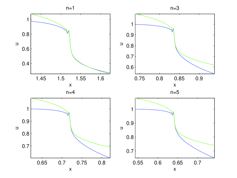
Fig. 1: The blue line is the solution of the generalized KdV equation $u_{t}+6u^{n}u_{x}+\epsilon^{2}u_{xxx}=0$ for different values of $n$ for the initial data $\phi(x)=1/\cosh^{2}x$ and $\epsilon=10^{-3}$ at the time $t_{c}$ and near the point of gradient catastrophe $x_{c}$ of the Hopf solution (center of the figure). The green line is the multiscale approximation in terms of the PI2 solution.

The quality of the asymptotic description shows the expected scaling for smaller values of $\epsilon$ as can be seen on the left in Fig. 2.

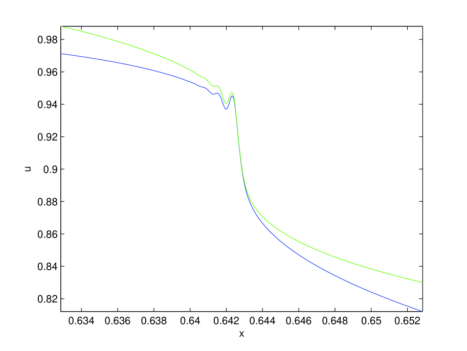
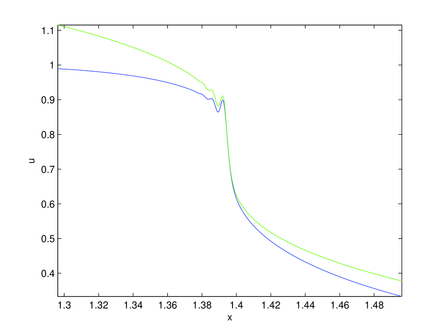
Fig. 2: The blue line is the solution of $u_{t}+a(u)u_{x}+\epsilon^{2}u_{xxx}=0$ with $a(u)=6u^{5}$ on the left and $a(u)=6\sinh u$ on the right, for the initial data $\phi(x)=1/\cosh^{2}x$ and $\epsilon=10^{-4}$ at the time $t_{c}$ near the point of gradient catastrophe $x_{c}$ of the Hopf solution (center of each figure). The green line is the multiscale approximation in terms of the PI2 solution.

The quality of this PI2 approximation is not limited to functions $a(u)$ in (5.43) which are polynomial in $u$. If we consider the case $a(u)=6\sinh u$, we obtain the right figure in Fig. 2. It can be seen that the PI2 asymptotics gives the same excellent description as for KdV.

5.2 Oscillatory regimes and blowup

It is known that solutions to initial value problems with sufficiently smooth initial data for the generalized KdV equation with $n<4$ are globally regular in time. This is not the case for for $n\geq 4$ where blowup can occur at finite time with $n=4$ being the critical case. For this case a theorem by Martel and Merle [24] states that solutions on the real line, with negative energy, blow up in finite or infinite time. For the general case $n>4$ and periodic settings considered here, the question is still open. Since the energy has the form

$$E=\int_{\mathbb{R}}\left[\frac{\epsilon^{2}}{2}u_{x}^{2}-\frac{6u^{n+2}}{(n+1)(n+2)}\right]\,dx$$

it will be always negative for sufficiently small $\epsilon$ and positive $u$.

Here we address numerically the question whether the formation of dispersive shocks, i.e., of a region of rapid modulated oscillations, precedes a potential blowup. We expect that the breakup of the solution to the dispersionless equation is regularized by the dispersion in the form of oscillations which then develop into blowup if the latter exists. This is exactly what we see in the following. Notice that the breakup time is given by the dispersionless equation and is thus independent of $\epsilon$. We first study the case $n=4$. For $\epsilon=1$, the energy is positive and no indication of blowup is observed. For $\epsilon=0.1$ we obtain for the initial data $\phi(x)=\mbox{sech}^{2}x$ the left figure in Fig. 3.

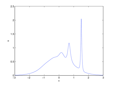
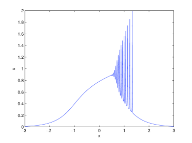
Fig. 3: Solution of the generalized KdV equation with $n=4$ for the initial data $\phi(x)=1/\cosh^{2}x$ and $\epsilon=10^{-1}$ at the time $t=0.3180\gg t_{c}$ on the left, and for $\epsilon=10^{-2}$ at the time $t=0.2235\gg t_{c}$ on the right.

For smaller $\epsilon$ ($\epsilon=0.01$) the behavior is similar, but there are as expected more oscillations, and the size of the oscillations reaches higher values earlier as can be seen in Fig. 3. For obvious reasons it is numerically difficult to decide whether the dispersive shock will lead to a blowup. In practice we run out of resolution before the code breaks down because of a blowup. This is due to oscillations in Fourier space as can be seen in Fig. 5. Though there is in principal enough resolution to approach $u(x,t)$, the oscillations of the Fourier coefficients make an accurate approximation via a Fourier transform impossible.

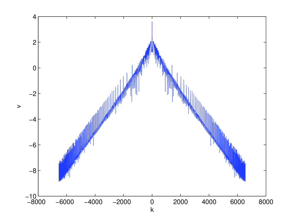
Fig. 4: Logarithm with base 10 of the modulus of the Fourier coefficents of the function shown in Fig. 3 on the right.

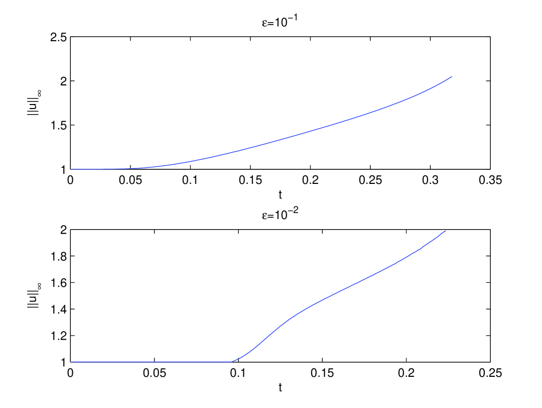
Fig. 5: $L^{\infty}$ norm of the solutions in Fig. 3.

The reason for this behavior is as discussed in [27] that singularities of the form $(z-z_{j})^{\mu_{j}}$ in the complex plane lead asymptotically to Fourier coefficients with modulus of the form $Ck^{-(\mu_{j}+1)}\exp(-\delta k)$, $\delta>0$. If there are several such singularities, there will be oscillations in the Fourier coefficients. In the present case there are at least two such singularities, the breakup which is strictly speaking only singular for $\epsilon=0$, but has an effect already for finite $\epsilon$, and the blowup, which leads to the behavior seen in (5). In Fig. 5 we give the $L^{\infty}$-norm of the solutions in Fig. 3. It cannot be decided on the base of these numerical data whether there is finite time blowup in this case. If it exists it is clearly preceded by a dispersive shock.

In the supercritical case $n=5$ we obtain a similar picture. In Fig. 6 we see the solution in the case $\epsilon=0.1$. Again it appears as if the rightmost peak evolves into a singularity.

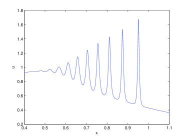
Fig. 6: Solution of the generalized KdV equation with $n=5$ for the initial data $\phi(x)=1/\cosh^{2}x$ and $\epsilon=10^{-1}$ at the time $t=0.2362\gg t_{c}$ on the left and for $\epsilon=10^{-2}$ at the time $t=0.2235\gg t_{c}$ on the right.

For smaller $\epsilon$ ($\epsilon=0.01$) there are again more oscillations, which stresses the importance of dispersive regularization before a potential blowup. Studying the $L^{\infty}$-norm of the solutions in Fig. 6, we can see that the case $\epsilon=0.1$ indeed seems to approach an $L^{\infty}$ blowup in finite time. Because of resolution problems we could not reach a similar point for $\epsilon=0.01$.

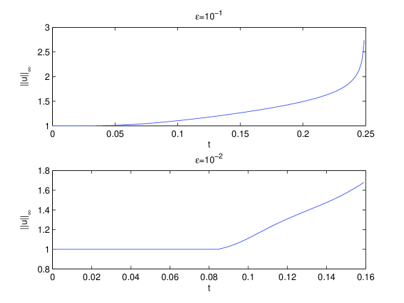
Fig. 7: $L^{\infty}$ norm of the solutions in Fig. 6.

6 Kawahara equations

The Kawahara equations [20] which appear in general dispersive media where the effects of the third order derivative is weak as in certain hydrodynamic or magneto-hydrodynamic settings can be written in the form

$$u_{t}+\frac{1}{2}\partial_{x}f(u,\epsilon\,u_{x},\epsilon^{2}u_{xx})+\beta\,\epsilon^{4}u_{xxxxx}=0.$$ (6.47)

Here we will mainly study the case

$$f(u,\epsilon\,u_{x},\epsilon^{2}u_{xx})=6u^{2}+2\alpha\,\epsilon^{2}u_{xx}$$ (6.48)

with $\alpha=1$ and $\beta=\pm 1$. The global well posedness of solutions of (6.47) in a suitable Sobolev space has been proved in [25].

The functional parameters $c(u)$, $p(u)$ in (2) are constants

$$c(u)=\frac{1}{6}\alpha,\quad p(u)=\frac{1}{12}\beta.$$ (6.49)

At the critical point we obtain for $\beta=-1$ that the breakup behavior is well described by PI2 in lowest order as can be seen in Fig. 8.

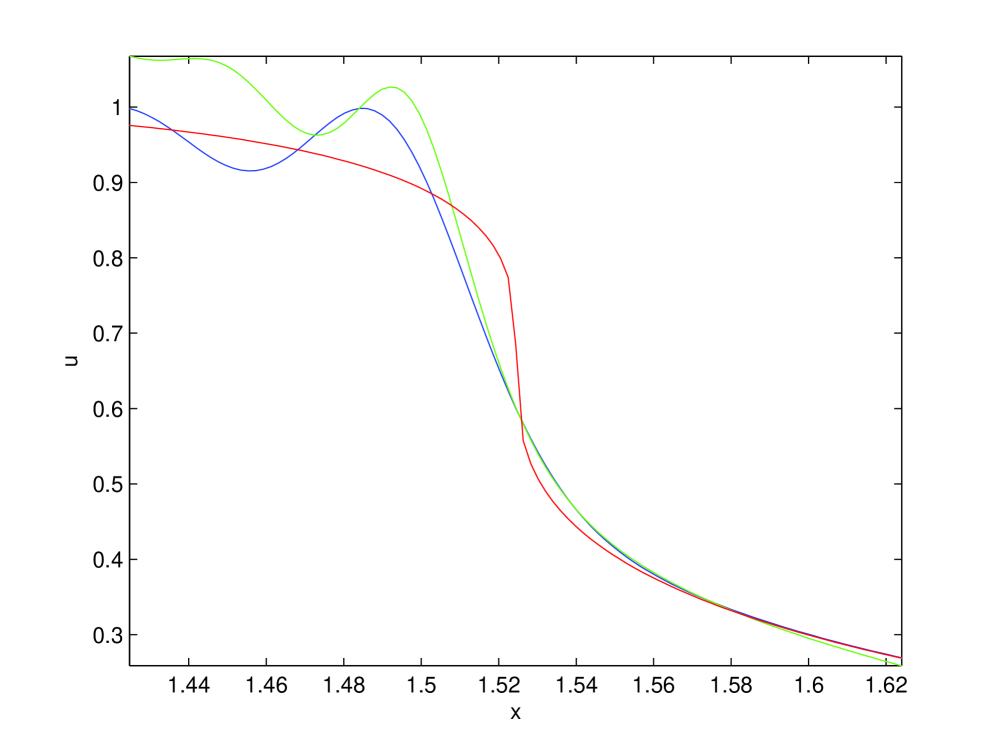
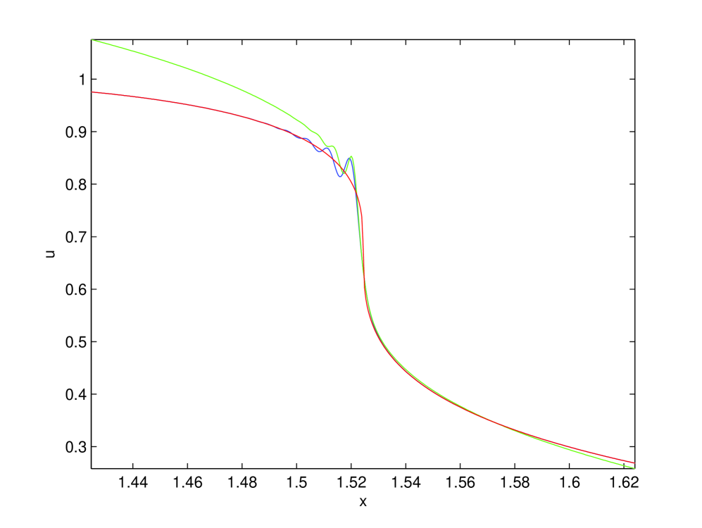
Fig. 8: The blue line is the solution of the Kawahara equation ($\beta=-1$) for the initial data $\phi(x)=1/\cosh^{2}x$ and $\epsilon=10^{-2}$ on the left figure and $\epsilon=10^{-3}$ on the right figure. The plot is taken at the time $t_{c}$ near the point of gradient catastrophe $x_{c}$ of the Hopf solution (center of the figure). Here $x_{c}\simeq 1.524$, $t_{c}\simeq 0.216$. The red line is the corresponding Hopf solution, the green line the multiscale approximation in terms of the PI2 solution.

It can be seen that the PI2 solution gives close to the breakup point a much better description of the Kawahara solution than the corresponding Hopf solution. The oscillation closest to the breakup point is too far away from the latter to be correctly reproduced, but the PI2 solution catches qualitatively the oscillatory behavior of the Kawahara solution near the critical point. With smaller $\epsilon$, the agreement gets as expected better, see the right figure in Fig. 8.

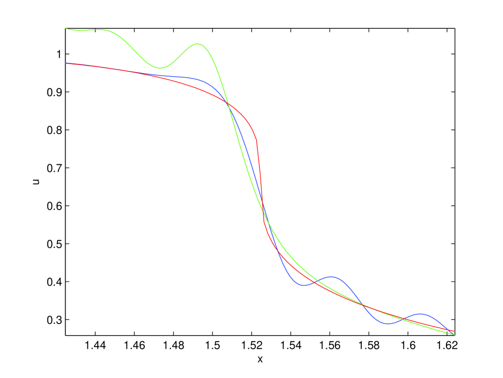
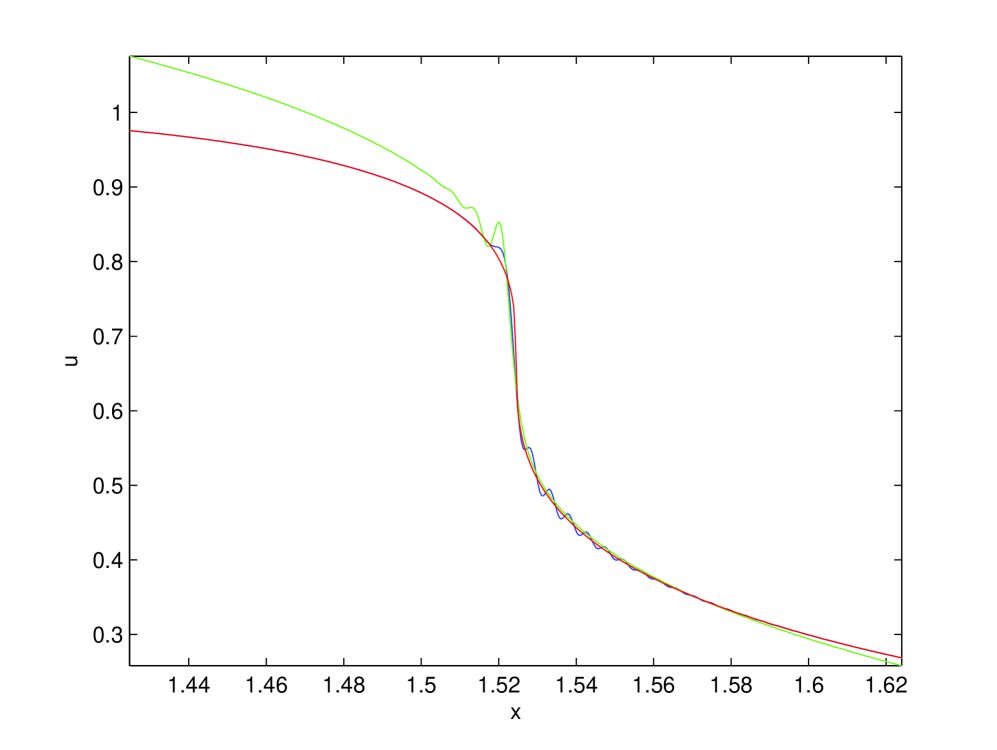
Fig. 9: The blue line is the solution of the Kawahara equation ($\beta=1$) for the initial data $\phi(x)=1/\cosh^{2}x$ and $\epsilon=10^{-2}$ on the left figure and $\epsilon=10^{-3}$ on the right figure. The plot is taken at the time $t_{c}$ near the point of gradient catastrophe $x_{c}$ of the Hopf solution (center of the figure). Here $x_{c}\simeq 1.524$, $t_{c}\simeq 0.216$. The red line is the corresponding Hopf solution, the green line is the multiscale approximation in terms of the PI2 solution.

For $\beta=1$, the breakup behavior of solutions to the Kawahara changes as can be seen from Fig. 9. In this case the oscillations in the Kawahara solution appear on the other side of the critical point and around it with small amplitude. This behaviour cannot be captured by the PI2 solution, but it is a higher order effect. Close to the critical point, the multiscale solution gives as before a much better description of the Kawahara solution than the Hopf solution.

For smaller values of $\epsilon$, both asymptotic solutions become more satisfactory as can be seen from the right figure in Fig. 9.

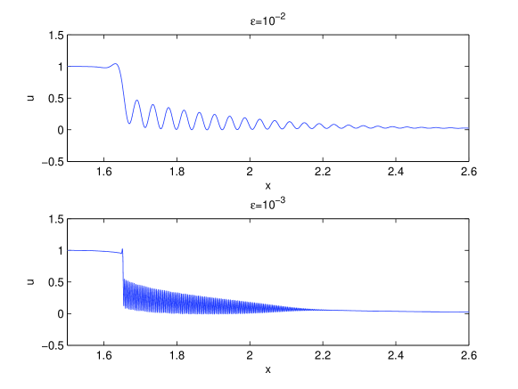
Fig. 10: Oscillatory zone of the solutions to the Kawahara equation ($\beta=1$) for the initial data $\phi(x)=1/\cosh^{2}x$ and two values of $\epsilon$ at time $t=0.25>t_{c}$.

It is interesting to notice that with decreasing $\epsilon$, the oscillations become smaller in amplitude in this case, but appear closer to the critical point. It can also be seen that the solution has the tendency to form one oscillation on the other side of the critical point close to the corresponding PI2 oscillation. Tracing the solution for larger times, it can be recognized that this will be the only oscillation to the left of the critical point, whereas a zone of high-frequent oscillations which appears to be essentially unbounded (see [18]) develops to the right, see Fig. 10. The oscillations appear to be as in the KdV case more and more confined to a zone similar to the Whitham zone, though no asymptotic description of the oscillations exists since the equation is not integrable.

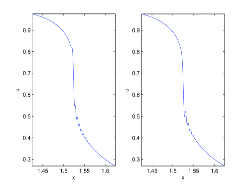
Fig. 11: Solutions of the Kawahara equation 6.47 with $\beta=1$ $\alpha=1$ to the left and $\alpha=0$ to the right. The solution is given for the initial data $\phi(x)=1/\cosh^{2}x$ and $\epsilon=10^{-3}$ at the time $t_{c}$ near the point of gradient catastrophe $x_{c}$ of the Hopf solution.

It seems also that this one oscillation to the left is really due to the third order derivative in the Kawahara equation as can be seen in Fig. 11 where one has to the left the Kawahara solution from Fig. 9 and to the right the analogous solution for $\alpha=0$, i.e., Kawahara without third order derivative. The oscillations to the right of the critical point being due to the fifth order derivative are present in both cases and have only slightly different form.

6.1 PDE with nonlinear dispersion

To show that the breakup behavior discussed in the previous sections is typical, we will now consider equations of the form (2.24) with nonlinear dispersion, i.e., with functions $c(u)$ and $p(u)$ not constant. The Camassa-Holm equation (CH) falls in this class if the nonlocal term is expanded in a von Neumann series, see [8], for functions $c(u)\sim u$ and $p(u)\sim u$. The applicability of the PI2 asymptotics to CH was studied numerically in [15]. For simplicity we restrict our analysis to the case $c(u)$ and $p(u)$ both proportional to $u^{2}$ with the Hopf equation as the dispersionless equation and initial data of the form $\phi(x)=\mbox{sech}^{2}x$. More complicated functions $c$ and $p$ can be considered, but the results are qualitatively the same.

In Fig. 13 the behavior at the critical time can be seen for $c(u)=u^{2}$ and $p(u)=0$. The situation is obviously as in the KdV case.

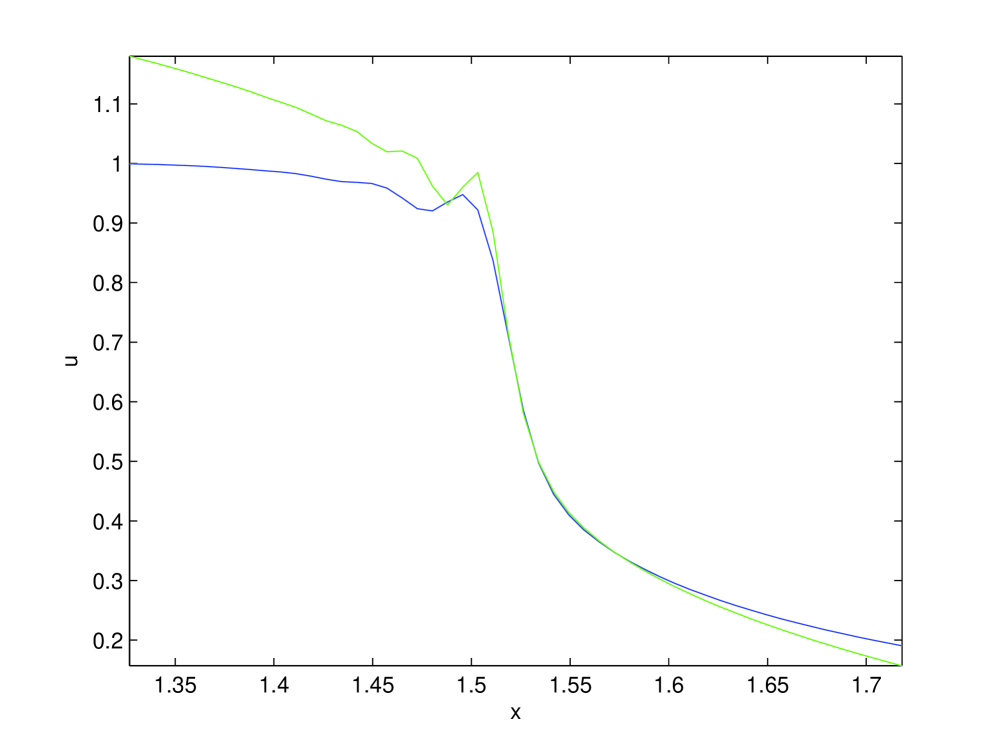
Fig. 12: Solution to the equation (2.24) for $a(u)=u$, $c(u)=u^{2}$ and $p(u)=0$ and initial data $\phi(x)=\mbox{sech}^{2}x$ at the critical time, and the corresponding multiscale solution in terms of the PI2 transcendent.

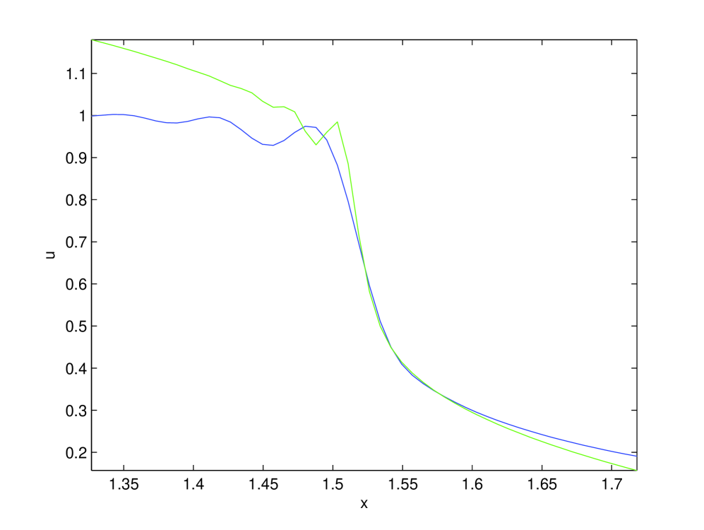
Fig. 13: Solution to the equation (2.24) for $a(u)=u$, $c(u)=-p(u)=u^{2}$ and initial data $\phi(x)=\mbox{sech}^{2}x$ at the critical time, and the corresponding multiscale solution in terms of the PI2 transcendent.

As for the Kawahara equation the relative sign between the third and the fifth derivative is important for the form of the oscillations. The situation with the opposite sign of $c$ and $p$ can be seen in Fig. 13. It is qualitatively the same as in the KdV case. New features appear as in the case of the Kawahara equation for the same sign in front of the third and fifth derivative. As can be seen in Fig. 14, oscillations of small amplitude appear as in the Kawahara equation on the other side of the critical point.

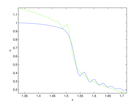
Fig. 14: Solution to the equation (2.24) for $a(u)=u$, $c(u)=p(u)=u^{2}$ and initial data $\phi(x)=\mbox{sech}^{2}x$ at the critical point, and the corresponding multiscale solution in terms of the PI2 transcendent.

Thus non constant functions $c(u)$ and $p(u)$ as expected do not change the picture from the case of constant functions as long as they do not vanish at the critical point.

6.2 Quasi-trivial transformation

In this subsection we study numerically the validity of the expansion given in sect. 4. For times $t\ll t_{c}$ the behavior of the solution of (4.34) should be described to order $\epsilon^{2}$ by the solution of the Hopf equation $u_{t}+uu_{x}=0$ with the same initial data. In fact we find that the difference between the Hopf solution and the solution to Kawahara equation (6.47) with $\beta=1$, $\alpha=1$ for the initial data $\phi(x)=\mbox{sech}^{2}x$ at $t=t_{c}/2$ scales as $\epsilon^{\gamma}$ with $\gamma=1.94$ (values of $\epsilon=10^{-1},10^{-1.125},\ldots,10^{-3}$, correlation coefficient $r=0.9997$ in linear regression, standard deviation $\sigma_{\alpha}=0.027$). For the same setting in the interval $x\in[0.8,2]$, the difference between the quasitriviality solution as described in sect. 4 and the Kawahara solution scales as $\epsilon^{\gamma}$ with $\gamma=3.77$ (correlation coefficient $r=0.999$ in linear regression, standard deviation $\sigma_{\alpha}=0.088$). This confirms the theoretical expectations. In Fig. 15 the difference between the Kawahara and the Hopf solution and the quasitriviality transform in order $\epsilon^{2}$ can be seen for this case. A similar scaling is observed for $\alpha=-1$ and $\alpha=0$ (KdV).

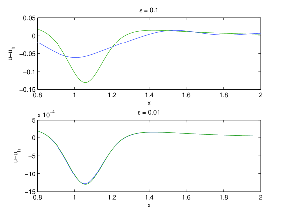
Fig. 15: Solution to the Kawahara equation with $\alpha=1$ for the initial data $\phi(x)=1/\cosh^{2}x$ at the time $t=t_{c}/2$ for two values of $\epsilon$; in blue the difference between the Kawahara and the corresponding Hopf solution, in green the order $\epsilon^{2}$ term of the quasitriviality transformation.

The difference between the solution of generalized KdV equation $u_{t}+u^{5}u_{x}+\epsilon^{2}u_{xxx}=0$ and the solution of the corresponding conservation law scales, at $t=t_{c}/2$ as $\epsilon^{\gamma}$ with $\gamma=1.9890$ (values of $\epsilon=10^{-1},10^{-1.125},\ldots,10^{-3}$, correlation coefficient $r=0.99998$ in linear regression, standard deviation $\sigma_{\alpha}=0.0068$).

6.3 Second equation in the KdV hierarchy

In this subsection we study the formation of dispersive shock waves for a family of equations that includes integrable and non-integrable PDEs. Interestingly the family of equations

$$u_{t}+30u^{2}u_{x}+10\alpha\epsilon^{2}(uu_{xxx}+2u_{x}u_{xx})+\epsilon^{4}u_{xxxxx}=0$$ (6.50)

having the invariants

$$c(u)=\frac{1}{6}\alpha,\quad p(u)=\frac{1-\alpha^{2}}{120u}$$

is completely integrable for $\alpha=\pm 1$ and coincides with the second equation in the KdV hierarchy (KdVII). Varying this factor one can study the transition to the Kawahara equation. As expected KdVII shows similar oscillations as KdV [14], as can be seen Fig. 16.

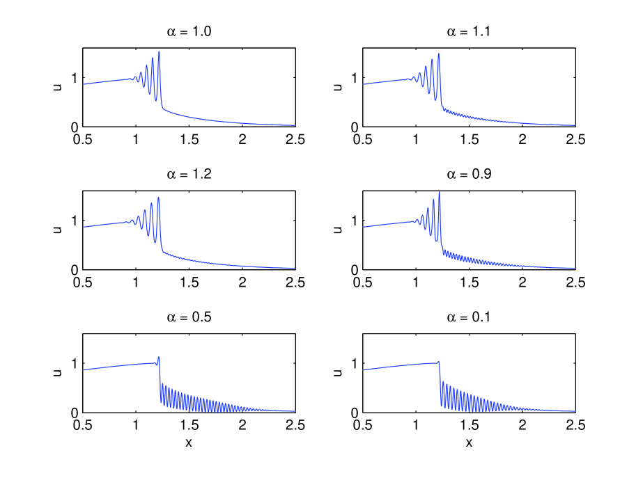
Fig. 16: Oscillatory part of the solution to the KdVII equation for the initial data $\phi(x)=1/\cosh^{2}x$ and $\epsilon=10^{-2}$ at a time $t=0.04>t_{c}=0.029$ for several values of $\alpha$.

For larger values of $\alpha$ one can recognize in Fig. 16 also a formation of oscillations on the other side of the inflection point as in the Kawahara equation. These effects become smaller for larger values of $\alpha$ ($\alpha>1.2$), but it shows that the phenomenon of integrability with the appearance of KdV-type oscillations is rather subtle. Thus it seems that the decisive factor for the appearence and the size of these oscillations is the relative sign and size of the factors in front of the third and the fifth derivative in the equation. Notice that equation (6.50) is for smaller $\alpha$ closer to the non-integrable (in higher orders in $\epsilon$) equation

$$u_{t}+30u^{2}u_{x}+\epsilon^{4}u_{xxxxx}=0$$

(see Section 3 above). It would be interesting to elaborate this observation in order to develop numerical tests of (approximate) integrability based on the study of the phase transition from regular to oscillatory behaviour.

Appendix A Numerical Methods

In this appendix we will briefly review the used methods in the numerical study of the PDE in the small dispersion limit and of the PI2 solution and give references in which details can be found.

Since critical phenomena are generally believed to be independent on specific boundary conditions, we restrict our analysis to essentially periodic functions. Typically we consider Schwarzian functions on a domain on which the functions are at the boundaries smaller than machine precision ($10^{-16}$ in double precision). Such functions can be periodically continued and are smooth with numerical precision. This allows a Fourier discretization of the spatial variables and an approximation of the solutions via truncated Fourier series. The use of Fourier spectral methods is especially efficient for the studied dispersive PDE because of the excellent approximation of smooth functions and the only minimal introduction of numerical dissipation. The latter is especially important if one is interested in the study of dispersive effects.

After discretization of the spatial coordinates, the PDE is equivalent to a typically large system of ordinary differential equations (ODE) in the time variable. Because of the high order of the spatial derivatives and because of the strong gradients we want to study, these systems will be typically stiff. If the stiff part is linear as is the case for the generalized KdV equations and for the Kawahara equations, the system of ODE has the form

$$Lv+N[v]=0,$$

where $v$ is the discrete Fourier transform of the solution, where $L$ is the stiff linear operator, and where the nonlinear term $N[v]$ contains only derivatives of lower order. For such systems, efficient integration schemes exist. We use a fourth order exponential time differencing scheme [6], see [21] for a comparison of fourth order schemes for KdV. The numerical accuracy is controlled by sufficient spatial resolution, i.e., Fourier coefficients decreasing to at least $10^{-8}$, and by numerically checking energy conservation. Since all equations studied here are Hamiltonian, energy is a conserved quantity. Due to unavoidable numerical errors, it will be weakly time dependent in numerical time integrations. As discussed in [21], conservation of the numerically computed energy typically overestimates the accuracy of a solution by two orders of magnitude. We always compute with an error in energy conservation smaller than $10^{-6}$ which implies that the error is well below plotting accuracy.

The situation is different for the equations with nonlinear dispersion in sect. 6.2. For these PDE we use an implicit fourth order Runge-Kutta method (Hammer and Hollingsworth method). These equations are numerically much more demanding. Therefore we compute with lower spatial resolution and an energy conservation of the order of $10^{-4}$.

The special solution of the PI2 equation is generated with the code bvp4 distributed with Matlab. For details see [15]. The Hopf solution is obtained from the implicit form $u(x,t)=\phi(\xi)$, $x=t\phi(\xi)+\xi$ with a fixed point iteration to machine precision. The derivatives of the Hopf solution are obtained by evaluating the the analytic expressions following from the characteristic method.

References

- [1] É.Brézin, E.Marinari, G.Parisi, A nonperturbative ambiguity free solution of a string model. Phys. Lett. B 242 (1990) 35–38.
- [2] Yu.A. Berezin, V.I. Karpman, On nonlinear evolution of perturbations in plasma and other dispersive media, Sov. Phys. JETP 22 (1966) 361.
- [3] P. Bleher, A. Its, Asymptotics of the partition function of a random matrix model. Ann. Inst. Fourier (Grenoble), 55, (2005), no. 6, 1943-2000.
- [4] T. Claeys, T. Grava, Universality of the break-up profile for the KdV equation in the small dispersion limit using the Riemann–Hilbert approach, arXiv:0801.2326, Comm. Math. Phys. 286 (2009) 979–1009.
- [5] T. Claeys, M. Vanlessen, The existence of a real pole-free solution of the fourth order analogue of the Painlevé I equation. Nonlinearity 20 (2007), no. 5, 1163–1184.
- [6] S. Cox and P. Matthews, Exponential time differencing for stiff systems, J. Comp. Phys. 176 (2002), pp. 430-455.
- [7] P. Dedecker and W.M. Tulczyjev, Spectral sequences and the inverse problem of the calculus of variations, Lecture Notes in Math. 836 (1980) 498-503.
- [8] B. Dubrovin, On Hamiltonian perturbations of hyperbolic systems of conservation laws, II: universality of critical behaviour, Comm. Math. Phys. 267 (2006) 117 - 139.
- [9] B. Dubrovin, On universality of critical behaviour in Hamiltonian PDEs, Amer. Math. Soc. Transl. 224 (2008) 59-109.
- [10] B. Dubrovin, Hamiltonian perturbations of hyperbolic PDEs: from classification results to the properties of solutions, In: New Trends in Mathematical Physics. Selected contributions of the XVth International Congress on Mathematical Physics, ed. V.Sidoravicius, Springer Netherlands, 2009., pp. 231-276.
- [11] B. Dubrovin, S.P. Novikov, Hydrodynamics of weakly deformed soliton lattices. Differential geometry and Hamiltonian theory. Russian Math. Surv. 44:6 (1989), 29-98.
- [12] N.Ercolani, K. McLaughlin, Asymptotics of the partition function for random matrices via Riemann-Hilbert techniques and applications to graphical enumeration. Int. Math. Res. Not., 14, (2003) 755-820.
- [13] J. Goodman, Zhou Ping Xin, Viscous limits for piecewise smooth solutions to systems of conservation laws. Arch. Rational Mech. Anal. 121 (1992), no. 3, 235-265.
- [14] T. Grava, C.Klein, Numerical solution of the small disperion limit of the KdV equation and Whitham equations, Comm. Pure Appl. Math. 60 (2007) 1623-1664.
- [15] T. Grava and C. Klein, Numerical study of a multiscale expansion of KdV and Camassa-Holm equation, in Integrable Systems and Random Matrices, ed. by J. Baik, T. Kriecherbauer, L.-C. Li, K.D.T-R. McLaughlin and C. Tomei, Contemp. Math. 458 (2008) 81-99.
- [16] A. Gurevich, L. Pitaevski, Nonstationary structure of a collisionless shock wave, Sov. Phys. JETP Lett. 38 (1974) 291–297.
- [17] T.Y. Hou, P.D. Lax, Dispersive approximations in fluid dynamics. Comm. Pure Appl. Math. 44 (1991) 1–40.
- [18] J.Hunter, J. Scheurle, Existence of perturbed solitary wave solutions to a model equation for water waves. Phys. D, 32 (1988), no. 2, 253-268.
- [19] A.A. Kapaev, Weakly nonlinear solutions of the equation , Zap. Nauchn. Sem. Leningrad. Otdel. Mat. Inst. Steklov. (LOMI) 187 (1991), Differentsialnaya Geom. Gruppy Li i Mekh. 12, 88–109, 172–173, 175; translation in J. Math. Sci. 73 (1995), no. 4, 468–481.
- [20] T. Kawahara, Oscillatory solitary waves in dispersive media, J. Phys. Soc. Japan, 33 (1972), 260-264.
- [21] C. Klein, Fourth order time-stepping for low dispersion Korteweg-de Vries and nonlinear Schrödinger equation, ETNA 29, (2008) 116-135.
- [22] Y. Kodama, A. Mikhailov, Obstacles to asymptotic integrability, Algebraic aspects of integrable systems, 173–204, Progr. Nonlinear Differential Equations Appl., 26, Birkhäuser, Boston, MA, 1997.
- [23] V. Kudashev, B. Suleimanov, A soft mechanism for the generation of dissipationless shock waves, Phys. Lett. A 221 (1996) 204–208.
- [24] Y. Martel and F. Merle, Stability of Blow-Up Profile and Lower Bounds for Blow-Up Rate for the Critical Generalized KdV Equation, Ann. Math., 155, (2002), 235-280.
- [25] G. Ponce, Lax pairs and higher order models for water waves, J. Differential Equations, 102 (1993), 360-381.
- [26] B. Suleĭmanov, Onset of nondissipative shock waves and the “nonperturbative” quantum theory of gravitation. J. Experiment. Theoret. Phys. 78 (1994), 583–587; translated from Zh. Èksper. Teoret. Fiz. 105 (1994), no. 5, 1089–1097.
- [27] C. Sulem, P.-L. Sulem and H. Frisch, Tracing Complex Singularities with Spectral Methods, J. Comp. Phys. 50, (1983) 138-161.
- [28] N.Zabusky, M.Kruskal, Interaction of “solitons” in a collisionless plasma and the recurrence of initial states, Phys. Rev. Lett. 15 (1965) 2403.