The Complexity of Euclidian 2 Dimension Travelling Salesman Problem versus General Assign Problem, NP is not P

Abstract

This paper presents the differences between two NP problems. It focuses in the Euclidian 2 Dimension Travelling Salesman Problems and General Assign Problems. The main results are the triangle reduction to verify the solution in polynomial time for the former and for the later the solution to the Noted Conjecture of the NP-Class, NP is not P.

Algorithms, NP, Numerical optimization.

1 Introduction

In [2] there are a complete introduction to this subject, an analysis in order to verify a solution for the Euclidian 2 Dimension Travelling Salesman Problem (E2DTSP) and the General Assign Problem (GAP). A review of the results for the travelling Salesman Problem is in [3], and for the NP Problems is in [4]

The next proposition is the key of this research: Given an arbitrary and large GAP_n, it has not an polynomial algorithm for verifying its solution.

Here a slight different approach is presented to differentiate and focuses only in the classes E2DTSP and GAP in order to determine that does nos exist a polynomial time algorithm for solving the later, i.e., there is not a polynomial time algorithm for solving the Hard NP problems. The notation, results and a more details are in [2].

Section 2 depicts the similarities, characteristics and propositions of the GAP_n and the E2DTSP_n. The main result is that an arbitrary and large E2DTSP_n preserves the inhered by construction the triangle inequality property. On the other hand, GAP_n does not preserve or inhere any property that could drive toward the construction of a verifying algorithm of its solution. Therefore, it is impossible to build an efficient algorithm for solving arbitrary and large GAP_n.The last section contains conclusions and future work.

2 The General Assign Problem and the Euclidian 2 Dimension Travelling Salesman Problem

The notation is the same as in [2].

Definition 2.1.

Notation

1. GAP_n is the General Assign Problem of size $n$.

2. E2DTSP_n stands for the version of the Traveller Salesman Problem with _n vertices. They come from points in a plane (as subset of $\mathbb{R}^{2}$) and the weight of the edges are the euclidian distance between vertices.

In this section the GAP_n and E2DTSP_n s characteristics and properties are presented. It is intended to give general results for TSP_n and for the specific case E2DTSP_n.

The GAP_n consists a complete graph, a function which assigns a value for each edge, and objective function, $\text{GAP}\_n$ $=$ $(G_{n},c,f)$, where $G_{n}=\left(V_{n},A\right)$, $V_{n}$ $\subset$ $\mathbb{N}$ $A$ $=$ $\left\{\left(i,j\right)\,|\,i,j\in V\right\}$, $c:V\times V\rightarrow\overline{\mathbb{R}}$, and $f$ is a real function for the evaluation of any path of vertices. Solving a GAP means to look for a minimum or a maximum value of $f$ over all cycles of $G_{n}$. Note that $c(i,i)=\inf$, and $c(\cdot,\cdot)$ can be see as a matrix of $\overline{\mathbb{R}}^{\,n\times n}.$

Remark 2.2.

Some properties and characteristics GAP and E2DTSP are:

1. The complete property of $G_{n}$ means that $\forall i,j\in V_{n},\exists e=(i,j)\in A$.

2. $G_{n}$ is a directed graph, which means that edges are a ordered pair.

3. A path of vertices is a sequence of vertices of $V_{n}$.

4. A cycle is a path of different vertices but the first and the last vertex are the same. Hereafter, a complete cycle is a cycle containing the $n$ vertices of $V_{n}$. Also, a complete cycle has $n$ edges.

5. A E2DTSP_n is a case of a GAP_n where $c(i,j)=c(j,i)$ (the cost matrix is symmetric) and $c(i,j)\geq 0,\forall i,j$, and finally $f$ is the sum of the edges’ cost of a cycle. It is a special case where $c(i,j)=\hbox{distance}(v_{i},v_{j})$ $\forall v_{i},v_{j}\in V_{n}$, the vertex $v_{i}\in\mathbb{R}^{2},\forall i=1,\ldots,n$, and $\hbox{distance}(v_{i},v_{j})=\|v_{i}-v_{j}\|$, is the Euclidian distance. Note that for a E2DTSP_n, we are going to refers to a vertex by its number or by $v_{i}$, in this case $v_{i}$ is a point of $\mathbb{R}^{2}$.

6. A sequence of vertices is a path and its denoted by $p_{k}$.

7. The objective function $f$ is also denoted by $c$, and let $c(p)$ be the cost function of the path $p$, i.e., it is given by the summation of edge s cost of the consecutive pairs of vertices of $p$.

The following propositions are easy to prove and they are well known results (also they are presented in [2]).

Proposition 2.3.

1. Any GAP_n has a solution. This means that exists a Hamiltonian cycle with minimum cost.

2. Let $f$ be the minimum or maximum edge s cost as the objective function. Then the Hamiltonian cycle of the GAP_n which is the solution can be found in polynomial time.

3. Any GAP_n has

   1. $n(n-1)$ edges.

   2. $(n-1)!$ complete cycles. The complete cycles can be enumerated in $n$ different ways. Hereafter, a cycle means a complete cycle.

   3. For $n\geq 4$, the maximum number of coincident edges of two different complete cycles is (n-3).

4. The Research Space of GAP_n is finite and numerable, and it has $(n-1)!$ elements and can be enumerated in $n$ different ways.

5. Let be $[i_{k}]_{k=1}^{n+1}$ a given cycle of a GAP_n. Then $\exists$! $m:[1,\ldots,n]\rightarrow[1,\ldots,n]$ such that the cost of the cycles do not change for an equivalent GAP’_n with cost function given by $c\circ m^{-1}=c(m^{-1}(\cdot))$ and $[m(i_{k})]_{k=1}^{n+1}=[n,n-1,\ldots,1,n]$, which corresponds to the first cycle of the descent enumeration of the vertices beginning with $n$.

6. Let be $[i_{k}]_{k=1}^{n+1}$ the solution cycle of a GAP_n. Then $\exists$! $m:[1,\ldots,n]\rightarrow[1,\ldots,n]$ such that $[n,n-1,\ldots,1,n]$ is the solution of the equivalent GAP_n, which corresponds to the first cycle of the descent enumeration of the vertices beginning with $n$.

7. Let be GAP_n such that $c(i,j)$ is given by the following matrix

   $$\left\{\begin{array}[]{ c c c c c}&1&2&\cdots&n-1\\ n&&n\cdot 2&\cdots&n\cdot n-1\\ \vdots&\vdots&\vdots&\vdots&\vdots\\ n^{n-2}&n^{n-2}\cdot 2&\cdots&&n^{n-2}\cdot(n-1)\\ n^{n-1}&n^{n-1}\cdot 2&\cdots&n^{n-1}\cdot(n-1)&\\ \end{array}\right\}$$

   then it has a unique solution and all cycles have different cost.

Important differences between GAP_n and TSP_n are in the following proposition. Here $c$ denotes de objective function.

Proposition 2.4.

1. For E2DTSP_n, $c$ is monotonically increasing,i.e, $c(p_{1})\leq c(p_{2})$ where the sequence of vertices of $p_{1}$ is a subsequence of $p_{2}$.

2. For GAP_n, $c$ is not monotonically increasing.

3. Let $c^{\prime}\in\mathbb{R}$, then for any E2DTSP_n, $P(c(p_{2})\geq c^{\prime}|c(p_{1})=c^{\prime})=1$ where $P$ is the probability function, and $p_{1}$ is a sub-path of $p_{2}$.

4. Let $c^{\prime}\in\mathbb{R}$, then for GAP_n. $P(c(p_{2})\leq c^{\prime}|c(p_{1})=c^{\prime})>0$ where $P$ is the probability function, and $p_{1}$ is a sub-path of $p_{2}$.

The following propositions characterizes the probability of searching the solution by a uniform random search. GAP has $n+1$, ($n$ very large) vertices in order to simplify the notation of the results.

Proposition 2.5.

Given an arbitrary and large GAP_n+1. Let be $m=\min\{c(j)\,|\,j\hbox{\, is a cycle of GAP}_{n+1}\}.$

1. The probability of selecting a cycle $j$ of GAP_n+1 is $P(j)=\frac{1}{n!}$.

2. $\frac{1}{n!}\leq P(j\,|\,c(j)\leq m)$. If GAP_n+1has a unique solution, $j$, then $P(j\,|\,c(j)\leq m)=\frac{1}{n!}.$

3. Let be $J$ a set of cycles of GAP_n+1, and cardinality of $|J|=n^{3},i.e.,|J|\sim\mathbf{O}((n+1)^{3})$. Then $\exists A,1<A<2^{3}$ such that $\frac{1}{A(n-3)!}\leq P(J)=\frac{n^{3}}{n!}\leq\frac{1}{n!}.$ Also, $\frac{(n-3)!-1}{(n-3)!}\leq P(J^{c})\leq\frac{A(n-3)!-1}{A(n-3)!}.$ This means $P(J)\approx 0,$ and $P(J^{c})\approx 1$.

Proof.

1. It follows from the basic properties of complete graph of GAP_n+1.

2. It follows by the previous statement and the unique $p_{j}$.

3. It follows from an appropriate approximation of $\frac{n!}{n^{3}}$.

∎

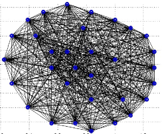
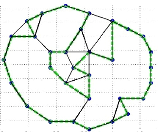
Figure 1: Example of a E2DTSP_n Complete and its triangle reduction.

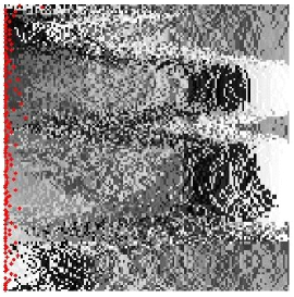
Figure 2: Example of the sorted cost matrix for E2DTSP_n Complete and its triangle reduction.

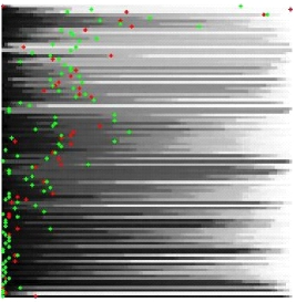
Figure 3: Sorted cost matrix for a GAP_n. The green dots are the solution. The red dots are a very closed solution

The last proposition shows that the cycle with minimum cost is quite difficult to find it, when no other properties are used than a uniform random search. Moreover, also if the solution is in a set of Hamiltonian cycles with polynomial cardinality, to look for it has a probability almost null, and the complementary event is almost certain. It means that properties are need to trim the search space in order to estimate or to verify the solution. The main difference between GAP_n and E2DTSP_n is that the last one preserve a triangle reducibility property. In [2] the reducibility was described for tubes, here, this property is related triangulation containing the solution. Fig. 1 depicts an example of this cunning property of an E2DTSP_n. Fig. 2 depicts the corresponding sorted cost matrix of an of the E2DTSP_n. Note that the triangle reduced sorted cost matrix is elongated, implying there are very few cycles to verify the solution.

Proposition 2.6.

Given any E2DTSP_n it is triangle reducible, i.e, it exists a triangulation of the E2DTSP which preserve the solution.

Proof.

Because the graph s edge’s values of the E2DTSP_n come from distances between vertices, it is trivial to build a triangulation for any E2DTSP_n over the Hamiltonian cycle which is the solution. Moreover, the triangle inequality permits to select the proper edges to avoid diagonal over the solution. This means that the reduced E2DTSP_n on this triangulation has the solution of the original problem by construction. ∎

In [2] a version of the previous proposition (Prop. 6.9) was presented to prove the that E2DTSP_n has an algorithm to verify the solution in polynomial time.

The next proposition shows that any E2DTSP_n combined with any GAP_m loss any property when they are combined to create a large GAP_n+m. Moreover, the class E2DTSP is a proper subset of the class GAP_n, i.e., class E2DTSP $\subset$ class GAP, and class GAP $\neq$ class E2DTSP.

Proposition 2.7.

Given a E2DTSP_n (which is triangle reducible) and a GAP_m, then $\exists$ a large arbitrary GAP_n+m which is not triangle reducible.

Proof.

The complete graph of a GAP_n+m is builded by inserting appropriately the graphs of E2DTSP_n and GAP_m. The rest of edges for the $n+m$ vertices can be added with random values. Finally, the resulting GAP_n+m is not reducible because many of its edges values are not from 2D distance between vertices but random values. Moreover, the graph’s edge’s values of the GAP_n+m do not comply the triangle inequality. ∎

In similar way, we can state the following property of lacking a property to verify the solution in polynomial time for arbitrary and large GAP_n. Fig .3 depicts the sorted cost matrix of a GAP_n. Because of the connectivity of the vertices with similar edge’ cost, there is not a simple reduction of the GAP_n’s graph as in the case of the E2DTSP_n. Note that the fact that the sorted cost matrix is not reduced, this imply that even with a putative solution there are many cycles to compare to verify the optimality of the putative solution.

Proposition 2.8.

Let be GAP_n, such that has an algorithm to verify the solution in polynomial time. Given any GAP_m, then $\exists$ a large arbitrary GAP_n+m which has not an algorithm to verify the solution in polynomial time.

Proof.

The complete graph of a GAP_n+m is builded by combining appropriately the graphs of GAP_n and GAP_m. The rest of edges for the $n+m$ vertices can be added with random values. The GAP_n’s algorithm provides a reduction of the edges of GAP_n to consider its solution to get a path, but the resulting GAP_n+m can change the path so the solution of GAP_n is not a sub path of the solution of GAP_n+m.

By example, it is possible to join GAP_n with two GAP${}_{\frac{m}{2}}$, in the way that GAP_n is like a tube. This case could preserve the solution of GAP_n but it is not a general case. Tt is easy to see by inspection of the sorted cost matrix M that the solution of GAP_n which it is founded by the polynomial time algorithm must comply to have a elongated reduction with an appropriate enumeration of the vertices, otherwise the verification of this solution it is not possible in polynomial time. This means, that only an appropriate and few edges are needed to consider for GAP_n. However, with an arbitrary joining between GAP_n and GAP_m a lot of edges with an appropriately random values not necessarily comply with the property (if it has one) of the verifying algorithm of GAP_n. In the arbitrary case it is possible that any vertices of GAP_n can have better alternatives by the added edges’ connection with the vertices of GAP_m. By alternatives, it is not only in the sense of a greedy algorithm, here we can have a sequences of oscillating edges’ random values. Therefore, it exists a GAP_n+m such that it nullifies or overrules any property inhered by the polynomial time algorithm of GAP_n for verifying the solution in polynomial time of GAP_n+m by the addition of appropriately random values for its edges. ∎

The proposition shows that an algorithm could claim and maybe solve a NP problem but the verification without properties over an a worst case with arbitrary data can not be demonstrated or seeing in polynomial time or by inspection of the sorted cost matrix M, and if the research space could be reduced then input problem is not a arbitrary worst case with many oscillating cycles. Prop. 2.4 states why E2DTSP_n’s solution is easy to verify but GAP_n.

Proposition 2.9.

Given an arbitrary and large GAP_n, it has not an polynomial algorithm for verifying its solution.

Proof.

It is immediately from the previous proposition. ∎

Conclusions and future work

Here the property of reduction was extended to triangle reduction for E2DTSP_n. This means that these are easy to verify the solution (and it is very possible to solve they in polynomial time) but arbitrary GAP_n is not. As it stated in [1] a triangulation algorithms has $\mathbf{O}\left(n^{\frac{m-1}{p}}\right)$, $\forall p\in[2,m-1]$. Therefore, it is highly possible that it exists an algorithm to solve arbitrary and large E2DTSP_n. However, the proposition 2.8 shows that arbitrary and large GAP_n, has not an inherited property allowing to build an efficient algorithm for verifying the solution, moreover, to solving it. When there is not structure or properties the simple machine, the finite automata has not an efficient implementation as it described in [2].

To my best knowledge this approach to verify in polynomial time the solution is given by the frontier’s position on the sorted cost matrix $\mathcal{M}$. The figures here depicts the differences between E2DTSP_n and GAP_n. The main result is from proposition 2.8, which is the base of the argumentation why P-Class (represented by E2DTSP_n) and the Hard NP-Class (represented by GAP_n) have totally different complexity. The later has not polynomial complexity in the general or worst case scenario, i.e., for large and arbitrary GAP_n but exponential. The result shows that does not exist a general property that allows to solve in polynomial time all Hard NP problems.

For the future, no student or colleague have accepted my invitation to build the efficient algorithm for E2DTSP_n using my results and by example the article [1] for building a triangulation.

Finally, this closing my previous article [2] in order to solve the Noted Conjecture of the NP-Class, and I hope, it brings a promising theoretical perspective to address the construction of efficient algorithms for arbitrary NP problems.

References

- [1] N. Amenta, D. Attali, and O. Devillers. Complexity of delaunay triangulation for points on lower-dimensional polyhedra. In SODA ’07: Proceedings of the eighteenth annual ACM-SIAM symposium on Discrete algorithms, pages 1106–1113, Philadelphia, PA, USA, 2007. SIAM.
- [2] C. Barrón-Romero. The complexity of the np-class. ArXiv, pages arXiv:submit/0056904, [cs.CC] 11 Jun 2010, 2010.
- [3] R. B. D. Applegate and V. Chvatal. On the solution of traveling salesman problems. In Documenta Mathematica Journal, Journal der Deutschen Mathematiker-Vereinigung, International Congress of Mathematicians, volume III, pages 645–656, 1998.
- [4] G. J. Woeginger. Exact algorithms for np-hard problems: A survey. Combinatorial Optimization - Eureka, You Shrink!, LNCS, pages 185–207, 2003.