Abstract.
Do there exist circular and spherical copulas in ℝ d superscript ℝ 𝑑 \mathbb{R}^{d} ℝ 2 superscript ℝ 2 \mathbb{R}^{2} ℝ d superscript ℝ 𝑑 \mathbb{R}^{d} d ≥ 3 𝑑 3 d\geq 3 d = 2 𝑑 2 d=2 d ≥ 4 𝑑 4 d\geq 4 ℝ 2 superscript ℝ 2 \mathbb{R}^{2} ℝ d superscript ℝ 𝑑 \mathbb{R}^{d} d = 2 𝑑 2 d=2
KEY WORDS AND PHRASES: Bivariate distribution, multivariate distribution, unit disk, unit ball, circular symmetry, spherical symmetry, circular copula, spherical copula, elliptical copula.
1. Introduction
Do there exist spherically symmetric distributions on the closed unit ball
B d subscript 𝐵 𝑑 B_{d} ℝ d superscript ℝ 𝑑 \mathbb{R}^{d} [ − 1 , 1 ] 1 1 [-1,1] B d subscript 𝐵 𝑑 B_{d} d = 2 𝑑 2 d=2 d ≥ 3 𝑑 3 d\geq 3
The cumulative distribution function (cdf) of a multivariate distribution
on the unit cube [ 0 , 1 ] d superscript 0 1 𝑑 [0,1]^{d} copula ; see
Nelsen (2006 ) for an accessible introduction to this topic. However, although it is
customary to confine attention to distributions on the unit cube,
our interest is in spherically symmetric (= orthogonally invariant)
distributions on B d subscript 𝐵 𝑑 B_{d}
Therefore we take “copula” to mean a multivariate cdf on the
centered cube C d := [ − 1 , 1 ] d assign subscript 𝐶 𝑑 superscript 1 1 𝑑 C_{d}:=[-1,1]^{d}
For d = 2 𝑑 2 d=2 d ≥ 3 𝑑 3 d\geq 3 circular copula (resp., spherical copula) if it is the cdf of a circularly symmetric (resp., spherically symmetric) distribution on the unit disk B 2 subscript 𝐵 2 B_{2} B d subscript 𝐵 𝑑 B_{d}
It will be noted in Sections 2 3 d = 2 𝑑 2 d=2 d = 3 𝑑 3 d=3 d ≥ 4 𝑑 4 d\geq 4 3 4
In Section 5 elliptical copulas is
obtained from the unique circular copula in ℝ 2 superscript ℝ 2 \mathbb{R}^{2} 6 ℝ d superscript ℝ 𝑑 \mathbb{R}^{d} d = 2 𝑑 2 d=2
3. The Bivariate Case: the Unique Circular Copula
The following three questions constitute an engaging classroom exercise.
Question 1. Let ( X , Y ) 𝑋 𝑌 (X,Y) B 2 subscript 𝐵 2 B_{2} ℝ 2 superscript ℝ 2 \mathbb{R}^{2} X 𝑋 X Y 𝑌 Y
Answer 1. One can easily show that X 𝑋 X
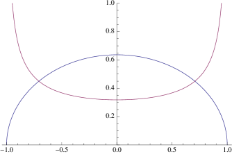
f ( x ) = 2 π 1 − x 2 , − 1 ≤ x ≤ 1 . formulae-sequence 𝑓 𝑥 2 𝜋 1 superscript 𝑥 2 1 𝑥 1 f(x)=\frac{2}{\pi}\sqrt{1-x^{2}},\quad-1\leq x\leq 1. (3.1)
(See Figure 1 Y 𝑌 Y X 𝑋 X
Question 2. Let ( X , Y ) 𝑋 𝑌 (X,Y) ∂ B 2 subscript 𝐵 2 \partial B_{2} ℝ 2 superscript ℝ 2 \mathbb{R}^{2} X 𝑋 X Y 𝑌 Y
Answer 2. We can represent ( X , Y ) 𝑋 𝑌 (X,Y) ( cos Θ , sin Θ ) Θ Θ (\cos\Theta,\,\sin\Theta) Θ ∼ uniform [ 0 , 2 π ) similar-to Θ uniform 0 2 𝜋 \Theta\sim{\rm uniform}[0,2\pi) X 𝑋 X
f ( x ) = 1 π 1 − x 2 , − 1 < x < 1 . formulae-sequence 𝑓 𝑥 1 𝜋 1 superscript 𝑥 2 1 𝑥 1 f(x)=\frac{1}{\pi\sqrt{1-x^{2}}},\quad-1<x<1. (3.2)
(See Figure 1 Y 𝑌 Y X 𝑋 X
Figure 1. The densities (3.1) (lower, blue) and (3.2) (upper, purple).
In both cases, the joint distribution of ( X , Y ) 𝑋 𝑌 (X,Y) ℝ 2 superscript ℝ 2 \mathbb{R}^{2} 1
Question 3. Does a circularly symmetric bivariate
distribution with uniform[ − 1 , 1 ] 1 1 [-1,1] B 2 subscript 𝐵 2 B_{2} C 2 subscript 𝐶 2 C_{2} 2.1 Bracewell (1986 ) .
Answer 3.
Optimistically, let’s seek an absolutely continuous solution.
That is, we seek a bivariate pdf on B 2 subscript 𝐵 2 B_{2}
f ( x , y ) = g ( x 2 + y 2 ) 𝑓 𝑥 𝑦 𝑔 superscript 𝑥 2 superscript 𝑦 2 f(x,y)=g(x^{2}+y^{2})
such that the marginal pdf
f ( x ) ≡ ∫ − 1 − x 2 1 − x 2 f ( x , y ) 𝑑 y , − 1 < x < 1 , formulae-sequence 𝑓 𝑥 superscript subscript 1 superscript 𝑥 2 1 superscript 𝑥 2 𝑓 𝑥 𝑦 differential-d 𝑦 1 𝑥 1 f(x)\equiv\int_{-\sqrt{1-x^{2}}}^{\sqrt{1-x^{2}}}f(x,y)dy,\qquad-1<x<1,
is constant in x 𝑥 x g 𝑔 g ( 0 , 1 ) 0 1 (0,1)
2 π ∫ 0 1 r g ( r 2 ) 𝑑 r = 1 2 𝜋 superscript subscript 0 1 𝑟 𝑔 superscript 𝑟 2 differential-d 𝑟 1 2\pi\int_{0}^{1}rg(r^{2})dr=1 (3.3)
in order that ∫ ∫ B 2 f ( x , y ) 𝑑 x 𝑑 y = 1 subscript subscript 𝐵 2 𝑓 𝑥 𝑦 differential-d 𝑥 differential-d 𝑦 1 \int\!\!\int_{B_{2}}f(x,y)dxdy=1 ( x , y ) → ( r , θ ) → 𝑥 𝑦 𝑟 𝜃 (x,y)\to(r,\theta)
To determine a suitable g 𝑔 g h ( t ) = g ( 1 − t ) ℎ 𝑡 𝑔 1 𝑡 h(t)=g(1-t) u = y 1 − x 2 𝑢 𝑦 1 superscript 𝑥 2 u=\frac{y}{\sqrt{1-x^{2}}}
f ( x ) 𝑓 𝑥 \displaystyle f(x) = \displaystyle= ∫ − 1 − x 2 1 − x 2 h ( 1 − x 2 − y 2 ) 𝑑 y superscript subscript 1 superscript 𝑥 2 1 superscript 𝑥 2 ℎ 1 superscript 𝑥 2 superscript 𝑦 2 differential-d 𝑦 \displaystyle\int_{-\sqrt{1-x^{2}}}^{\sqrt{1-x^{2}}}h(1-x^{2}-y^{2})dy
= \displaystyle= 1 − x 2 ∫ − 1 1 h ( ( 1 − u 2 ) ( 1 − x 2 ) ) 𝑑 u 1 superscript 𝑥 2 superscript subscript 1 1 ℎ 1 superscript 𝑢 2 1 superscript 𝑥 2 differential-d 𝑢 \displaystyle\sqrt{1-x^{2}}\int_{-1}^{1}h((1-u^{2})(1-x^{2}))du
= \displaystyle= 2 1 − x 2 ∫ 0 1 h ( ( 1 − u 2 ) ( 1 − x 2 ) ) 𝑑 u . 2 1 superscript 𝑥 2 superscript subscript 0 1 ℎ 1 superscript 𝑢 2 1 superscript 𝑥 2 differential-d 𝑢 \displaystyle 2\sqrt{1-x^{2}}\int_{0}^{1}h((1-u^{2})(1-x^{2}))du.
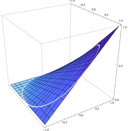
If we take h ( t ) = c t − 1 / 2 ℎ 𝑡 𝑐 superscript 𝑡 1 2 h(t)=c\,t^{-1/2} f ( x ) 𝑓 𝑥 f(x) x 𝑥 x c = 1 / 2 π 𝑐 1 2 𝜋 c=1/2\pi 3.3
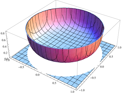
f ( x , y ) = 1 2 π 1 − x 2 − y 2 , x 2 + y 2 < 1 , formulae-sequence 𝑓 𝑥 𝑦 1 2 𝜋 1 superscript 𝑥 2 superscript 𝑦 2 superscript 𝑥 2 superscript 𝑦 2 1 f(x,y)=\frac{1}{2\pi\sqrt{1-x^{2}-y^{2}}},\qquad x^{2}+y^{2}<1, (3.4)
determines a circularly symmetric bivariate distribution on B 2 subscript 𝐵 2 B_{2}
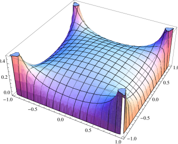
Figure 2. Circularly symmetric bivariate density on B 2 subscript 𝐵 2 B_{2}
Question 4. Having determined the unique circularly
symmetric distribution (3.4 B 2 subscript 𝐵 2 B_{2} F ( x , y ) 𝐹 𝑥 𝑦 F(x,y)
Answer 4.
The circular symmetry of ( X , Y ) 𝑋 𝑌 (X,Y) ( X , Y ) = d ( ± X , ± Y ) superscript 𝑑 𝑋 𝑌 plus-or-minus 𝑋 plus-or-minus 𝑌 (X,Y)\buildrel d\over{=}(\pm X,\,\pm Y) F ( x , y ) ≡ P [ X ≤ x , Y ≤ y ] 𝐹 𝑥 𝑦 𝑃 delimited-[] formulae-sequence 𝑋 𝑥 𝑌 𝑦 F(x,y)\equiv P[X\leq x,\,Y\leq y] C 2 ≡ [ − 1 , 1 ] 2 subscript 𝐶 2 superscript 1 1 2 C_{2}\equiv[-1,1]^{2} F 0 ( x , y ) subscript 𝐹 0 𝑥 𝑦 F_{0}(x,y)
F 0 ( x , y ) ≡ P [ 0 ≤ X ≤ x , 0 ≤ Y ≤ y ] F_{0}(x,y)\equiv P[0\leq X\leq x,\,0\leq Y\leq y] (3.5)
for 0 ≤ x , y ≤ 1 formulae-sequence 0 𝑥 𝑦 1 0\leq x,y\leq 1 F ¯ ( x , y ) ≡ P [ X > x , Y > y ] ¯ 𝐹 𝑥 𝑦 𝑃 delimited-[] formulae-sequence 𝑋 𝑥 𝑌 𝑦 \bar{F}(x,y)\equiv P[X>x,\,Y>y] 0 ≤ x , y ≤ 1 formulae-sequence 0 𝑥 𝑦 1 0\leq x,y\leq 1 ( X , Y ) = d ( ± X , ± Y ) superscript 𝑑 𝑋 𝑌 plus-or-minus 𝑋 plus-or-minus 𝑌 (X,Y)\buildrel d\over{=}(\pm X,\,\pm Y) [ − 1 , 1 ] 1 1 [-1,1]
F 0 ( x , y ) subscript 𝐹 0 𝑥 𝑦 \displaystyle F_{0}(x,y) = \displaystyle= P [ 0 ≤ X ≤ 1 , 0 ≤ Y ≤ 1 ] − P [ X > x , 0 ≤ Y ≤ 1 ] \displaystyle P[0\leq X\leq 1,\,0\leq Y\leq 1]-P[X>x,\,0\leq Y\leq 1] (3.6)
− P [ 0 ≤ X ≤ 1 , Y > y ] + P [ X > x , Y > y ] \displaystyle-P[0\leq X\leq 1,\,Y>y]+P[X>x,\,Y>y]
= \displaystyle= 1 4 − ( 1 − x 4 ) − ( 1 − y 4 ) + F ¯ ( x , y ) 1 4 1 𝑥 4 1 𝑦 4 ¯ 𝐹 𝑥 𝑦 \displaystyle\frac{1}{4}-\left(\frac{1-x}{4}\right)-\left(\frac{1-y}{4}\right)+\bar{F}(x,y)
= \displaystyle= x + y − 1 4 + F ¯ ( x , y ) , 0 ≤ x , y ≤ 1 . formulae-sequence 𝑥 𝑦 1 4 ¯ 𝐹 𝑥 𝑦 0
𝑥 𝑦 1 \displaystyle\frac{x+y-1}{4}+\bar{F}(x,y),\quad 0\leq x,y\leq 1.
Lemma 3.1 .
Let ( X , Y ) 𝑋 𝑌 (X,Y) C 2 subscript 𝐶 2 C_{2} [ − 1 , 1 ] 1 1 [-1,1] ( X , Y ) = d ( ± X , ± Y ) superscript 𝑑 𝑋 𝑌 plus-or-minus 𝑋 plus-or-minus 𝑌 (X,Y)\buildrel d\over{=}(\pm X,\,\pm Y) ( x , y ) ∈ C 2 𝑥 𝑦 subscript 𝐶 2 (x,y)\in C_{2}
F ( x , y ) 𝐹 𝑥 𝑦 \displaystyle F(x,y) = \displaystyle= x + y + 1 4 + σ ( x y ) F 0 ( | x | , | y | ) 𝑥 𝑦 1 4 𝜎 𝑥 𝑦 subscript 𝐹 0 𝑥 𝑦 \displaystyle\frac{x+y+1}{4}+\sigma(xy)\,F_{0}(|x|,|y|) (3.7)
= \displaystyle= x + y + 1 4 + σ ( x y ) [ | x | + | y | − 1 4 + F ¯ ( | x | , | y | ) ] , 𝑥 𝑦 1 4 𝜎 𝑥 𝑦 delimited-[] 𝑥 𝑦 1 4 ¯ 𝐹 𝑥 𝑦 \displaystyle\frac{x+y+1}{4}+\sigma(xy)\left[\frac{|x|+|y|-1}{4}+\bar{F}(|x|,|y|)\right], (3.8)
where σ ( w ) = sign ( w ) 𝜎 𝑤 sign 𝑤 \sigma(w)=\mathrm{sign}(w) w ≠ 0 𝑤 0 w\neq 0 σ ( 0 ) = 0 𝜎 0 0 \sigma(0)=0
Proof.
To obtain (3.7
Case 1: 0 ≤ x , y ≤ 1 formulae-sequence 0 𝑥 𝑦 1 0\leq x,y\leq 1 ( X , Y ) 𝑋 𝑌 (X,Y) [ − 1 , 1 ] 1 1 [-1,1]
F ( x , y ) 𝐹 𝑥 𝑦 \displaystyle F(x,y) = \displaystyle= P [ 0 < X ≤ x , 0 < Y ≤ y ] + P [ 0 < X ≤ x , Y ≤ 0 ] \displaystyle P[0<X\leq x,\,0<Y\leq y]+P[0<X\leq x,\,Y\leq 0]
+ P [ X ≤ 0 , 0 < Y ≤ y ] + P [ X ≤ 0 , Y ≤ 0 ] 𝑃 delimited-[] formulae-sequence 𝑋 0 0 𝑌 𝑦 𝑃 delimited-[] formulae-sequence 𝑋 0 𝑌 0 \displaystyle+P[X\leq 0,\,0<Y\leq y]+P[X\leq 0,\,Y\leq 0]
= \displaystyle= F 0 ( x , y ) + x 4 + y 4 + 1 4 subscript 𝐹 0 𝑥 𝑦 𝑥 4 𝑦 4 1 4 \displaystyle F_{0}(x,y)+\frac{x}{4}+\frac{y}{4}+\frac{1}{4}
= \displaystyle= x + y + 1 4 + σ ( x y ) F 0 ( | x | , | y | ) . 𝑥 𝑦 1 4 𝜎 𝑥 𝑦 subscript 𝐹 0 𝑥 𝑦 \displaystyle\frac{x+y+1}{4}+\sigma(xy)\,F_{0}(|x|,|y|).
Case 2: − 1 ≤ x ≤ 0 ≤ y ≤ 1 1 𝑥 0 𝑦 1 -1\leq x\leq 0\leq y\leq 1
F ( x , y ) 𝐹 𝑥 𝑦 \displaystyle F(x,y) = \displaystyle= P [ X ≤ 0 , 0 < Y ≤ y ] − P [ x < X ≤ 0 , 0 ≤ Y ≤ y ] \displaystyle\ \ P[X\leq 0,\,0<Y\leq y]-P[x<X\leq 0,\,0\leq Y\leq y]
+ P [ X ≤ 0 , Y ≤ 0 ] − P [ x < X ≤ 0 , Y ≤ 0 ] \displaystyle+P[X\leq 0,\,Y\leq 0]-P[x<X\leq 0,\,Y\leq 0]
= \displaystyle= y 4 − F 0 ( − x , y ) + 1 4 − ( − x ) 4 𝑦 4 subscript 𝐹 0 𝑥 𝑦 1 4 𝑥 4 \displaystyle\frac{y}{4}-F_{0}(-x,y)+\frac{1}{4}-\frac{(-x)}{4}
= \displaystyle= x + y + 1 4 + σ ( x y ) F 0 ( | x | , | y | ) . 𝑥 𝑦 1 4 𝜎 𝑥 𝑦 subscript 𝐹 0 𝑥 𝑦 \displaystyle\frac{x+y+1}{4}+\sigma(xy)\,F_{0}(|x|,|y|).
Case 3: − 1 ≤ y ≤ 0 ≤ x ≤ 1 1 𝑦 0 𝑥 1 -1\leq y\leq 0\leq x\leq 1
F ( x , y ) 𝐹 𝑥 𝑦 \displaystyle F(x,y) = \displaystyle= P [ 0 < X ≤ x , Y ≤ 0 ] − P [ 0 ≤ X ≤ x , y < Y ≤ 0 ] \displaystyle P[0<X\leq x,\,Y\leq 0]-P[0\leq X\leq x,\,y<Y\leq 0]
+ P [ X ≤ 0 , Y ≤ 0 ] − P [ X ≤ 0 , y < Y ≤ 0 ] 𝑃 delimited-[] formulae-sequence 𝑋 0 𝑌 0 𝑃 delimited-[] formulae-sequence 𝑋 0 𝑦 𝑌 0 \displaystyle+P[X\leq 0,\,Y\leq 0]-P[X\leq 0,\,y<Y\leq 0]
= \displaystyle= x 4 − F 0 ( x , − y ) + 1 4 − ( − y ) 4 𝑥 4 subscript 𝐹 0 𝑥 𝑦 1 4 𝑦 4 \displaystyle\frac{x}{4}-F_{0}(x,-y)+\frac{1}{4}-\frac{(-y)}{4}
= \displaystyle= x + y + 1 4 + σ ( x y ) F 0 ( | x | , | y | ) . 𝑥 𝑦 1 4 𝜎 𝑥 𝑦 subscript 𝐹 0 𝑥 𝑦 \displaystyle\frac{x+y+1}{4}+\sigma(xy)\,F_{0}(|x|,|y|).
Case 4: − 1 ≤ x , y ≤ 0 formulae-sequence 1 𝑥 𝑦 0 -1\leq x,y\leq 0
F ( x , y \displaystyle F(x,y ) = \displaystyle)= P [ X ≤ 0 , Y ≤ 0 ] − P [ x < X ≤ 0 , Y ≤ 0 ] \displaystyle P[X\leq 0,\,Y\leq 0]-P[x<X\leq 0,\,Y\leq 0]
− P [ X ≤ 0 , y < Y ≤ 0 ] + P [ x < X ≤ 0 , y < Y ≤ 0 ] \displaystyle-P[X\leq 0,\,y<Y\leq 0]+P[x<X\leq 0,\,y<Y\leq 0]
= \displaystyle= 1 4 − ( − x ) 4 − ( − y ) 4 + F 0 ( − x , − y ) 1 4 𝑥 4 𝑦 4 subscript 𝐹 0 𝑥 𝑦 \displaystyle\frac{1}{4}-\frac{(-x)}{4}-\frac{(-y)}{4}+F_{0}(-x,-y)
= \displaystyle= x + y + 1 4 + σ ( x y ) F 0 ( | x | , | y | ) . 𝑥 𝑦 1 4 𝜎 𝑥 𝑦 subscript 𝐹 0 𝑥 𝑦 \displaystyle\frac{x+y+1}{4}+\sigma(xy)\,F_{0}(|x|,|y|).
Finally, (3.8 3.7 3.6
Thus, to determine the circular copula F ( x , y ) 𝐹 𝑥 𝑦 F(x,y) 3.4 F ¯ ( x , y ) ¯ 𝐹 𝑥 𝑦 \bar{F}(x,y) 0 ≤ x , y ≤ 1 formulae-sequence 0 𝑥 𝑦 1 0\leq x,y\leq 1 3.8 F ¯ ( x , y ) = 0 ¯ 𝐹 𝑥 𝑦 0 \bar{F}(x,y)=0 x 2 + y 2 ≥ 1 superscript 𝑥 2 superscript 𝑦 2 1 x^{2}+y^{2}\geq 1 x 2 + y 2 < 1 superscript 𝑥 2 superscript 𝑦 2 1 x^{2}+y^{2}<1
First approach:
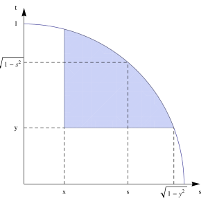
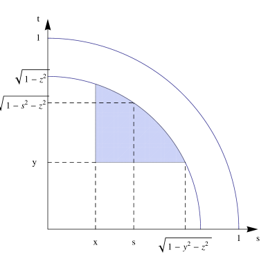
When 0 ≤ x , y ≤ 1 formulae-sequence 0 𝑥 𝑦 1 0\leq x,y\leq 1 x 2 + y 2 < 1 superscript 𝑥 2 superscript 𝑦 2 1 x^{2}+y^{2}<1 F ¯ ( x , y ) ¯ 𝐹 𝑥 𝑦 \bar{F}(x,y) 3
Figure 3. Region of integration, 2-dimensional case
F ¯ ( x , y ) ¯ 𝐹 𝑥 𝑦 \displaystyle\bar{F}(x,y) = \displaystyle= 1 2 π ∫ x 1 − y 2 { ∫ y 1 − s 2 1 1 − s 2 − t 2 𝑑 t } 𝑑 s 1 2 𝜋 superscript subscript 𝑥 1 superscript 𝑦 2 superscript subscript 𝑦 1 superscript 𝑠 2 1 1 superscript 𝑠 2 superscript 𝑡 2 differential-d 𝑡 differential-d 𝑠 \displaystyle\frac{1}{2\pi}\int_{x}^{\sqrt{1-y^{2}}}\left\{\int_{y}^{\sqrt{1-s^{2}}}\frac{1}{\sqrt{1-s^{2}-t^{2}}}dt\right\}ds (3.9)
= \displaystyle= 1 2 π ∫ x 1 − y 2 { ∫ y 1 − s 2 1 ( 1 − t 2 1 − s 2 ) d t 1 − s 2 } 𝑑 s 1 2 𝜋 superscript subscript 𝑥 1 superscript 𝑦 2 superscript subscript 𝑦 1 superscript 𝑠 2 1 1 superscript 𝑡 2 1 superscript 𝑠 2 𝑑 𝑡 1 superscript 𝑠 2 differential-d 𝑠 \displaystyle\frac{1}{2\pi}\int_{x}^{\sqrt{1-y^{2}}}\left\{\int_{y}^{\sqrt{1-s^{2}}}\frac{1}{\sqrt{(1-\frac{t^{2}}{1-s^{2}})}}\frac{dt}{\sqrt{1-s^{2}}}\right\}ds
= \displaystyle= 1 2 π ∫ x 1 − y 2 { ∫ y 1 − s 2 1 d v 1 − v 2 } 𝑑 s 1 2 𝜋 superscript subscript 𝑥 1 superscript 𝑦 2 superscript subscript 𝑦 1 superscript 𝑠 2 1 𝑑 𝑣 1 superscript 𝑣 2 differential-d 𝑠 \displaystyle\frac{1}{2\pi}\int_{x}^{\sqrt{1-y^{2}}}\left\{\int_{\frac{y}{\sqrt{1-s^{2}}}}^{1}\frac{dv}{\sqrt{1-v^{2}}}\right\}ds
= \displaystyle= 1 2 π ∫ x 1 − y 2 [ π 2 − arcsin ( y 1 − s 2 ) ] 𝑑 s . 1 2 𝜋 superscript subscript 𝑥 1 superscript 𝑦 2 delimited-[] 𝜋 2 𝑦 1 superscript 𝑠 2 differential-d 𝑠 \displaystyle\frac{1}{2\pi}\int_{x}^{\sqrt{1-y^{2}}}\left[\frac{\pi}{2}-\arcsin\left(\frac{y}{\sqrt{1-s^{2}}}\right)\right]ds.
However, we were unable to evaluate this integral directly.
Second approach:
Fortunately, we have found a solution in the molecular biology and optics literatures,
where the problem of finding the area of the intersection of two spherical caps on the
unit sphere ∂ B 3 subscript 𝐵 3 \partial B_{3} Tovchigrechko and Vakser (2001 ) and also appears in
Oat and Sander (2007 ) .
Lemma 3.2 .
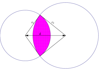
Let S 1 subscript 𝑆 1 S_{1} S 2 subscript 𝑆 2 S_{2} ∂ B 3 subscript 𝐵 3 \partial B_{3} r 1 subscript 𝑟 1 r_{1} r 2 subscript 𝑟 2 r_{2} d 𝑑 d 0 < d ≤ π 0 𝑑 𝜋 0<d\leq\pi 0 < r 1 , r 2 ≤ π / 2 formulae-sequence 0 subscript 𝑟 1 subscript 𝑟 2 𝜋 2 0<r_{1},r_{2}\leq\pi/2 d ≤ r 1 + r 2 𝑑 subscript 𝑟 1 subscript 𝑟 2 d\leq r_{1}+r_{2} S 1 ∩ S 2 ≠ ∅ subscript 𝑆 1 subscript 𝑆 2 S_{1}\cap S_{2}\neq\emptyset 4 5 ( S 1 ∩ S 2 ) subscript 𝑆 1 subscript 𝑆 2 (S_{1}\cap S_{2})
A ( r 1 , r 2 ; d ) 𝐴 subscript 𝑟 1 subscript 𝑟 2 𝑑 \displaystyle A(r_{1},r_{2};d) = \displaystyle= 2 π − 2 π cos ( r 1 ) − 2 π cos ( r 2 ) − 2 arccos ( cos ( d ) − cos ( r 1 ) cos ( r 2 ) sin ( r 1 ) sin ( r 2 ) ) 2 𝜋 2 𝜋 subscript 𝑟 1 2 𝜋 subscript 𝑟 2 2 𝑑 subscript 𝑟 1 subscript 𝑟 2 subscript 𝑟 1 subscript 𝑟 2 \displaystyle 2\pi-2\pi\cos(r_{1})-2\pi\cos(r_{2})-2\arccos\left(\frac{\cos(d)-\cos(r_{1})\cos(r_{2})}{\sin(r_{1})\sin(r_{2})}\right) (3.10)
+ 2 cos ( r 1 ) arccos ( cos ( d ) cos ( r 1 ) − cos ( r 2 ) sin ( d ) sin ( r 1 ) ) 2 subscript 𝑟 1 𝑑 subscript 𝑟 1 subscript 𝑟 2 𝑑 subscript 𝑟 1 \displaystyle+\ 2\cos(r_{1})\arccos\left(\frac{\cos(d)\cos(r_{1})-\cos(r_{2})}{\sin(d)\sin(r_{1})}\right)
+ 2 cos ( r 2 ) arccos ( cos ( d ) cos ( r 2 ) − cos ( r 1 ) sin ( d ) sin ( r 2 ) ) . 2 subscript 𝑟 2 𝑑 subscript 𝑟 2 subscript 𝑟 1 𝑑 subscript 𝑟 2 \displaystyle+\ 2\cos(r_{2})\arccos\left(\frac{\cos(d)\cos(r_{2})-\cos(r_{1})}{\sin(d)\sin(r_{2})}\right).
This result can be applied to obtain our desired circular copula as follows.
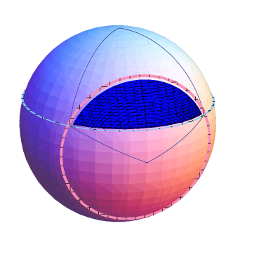
If ( X , Y , Z ) 𝑋 𝑌 𝑍 (X,Y,Z) ∂ B 3 subscript 𝐵 3 \partial B_{3} { X > x , Y > y } formulae-sequence 𝑋 𝑥 𝑌 𝑦 \{X>x,\,Y>y\} { X > x } 𝑋 𝑥 \{X>x\} { Y > y } 𝑌 𝑦 \{Y>y\} P [ X > x , Y > y ] 𝑃 delimited-[] formulae-sequence 𝑋 𝑥 𝑌 𝑦 P[X>x,\,Y>y] A ( x , y ) 𝐴 𝑥 𝑦 A(x,y) ∂ B 3 subscript 𝐵 3 \partial B_{3} 4 π 4 𝜋 4\pi 4 5 ( X , Y ) 𝑋 𝑌 (X,Y) B 2 subscript 𝐵 2 B_{2} 3.4
Figure 4. Intersection of two spherical capsFigure 5. Intersection of two spherical caps,
circular representation (modified from Tovchigrechko and Vakser (2001 ) )
Thus, for 0 ≤ x , y ≤ 1 formulae-sequence 0 𝑥 𝑦 1 0\leq x,y\leq 1 x 2 + y 2 < 1 superscript 𝑥 2 superscript 𝑦 2 1 x^{2}+y^{2}<1
F ¯ ( x , y ) ¯ 𝐹 𝑥 𝑦 \displaystyle\bar{F}(x,y) = \displaystyle= 1 4 π A ( x , y ) 1 4 𝜋 𝐴 𝑥 𝑦 \displaystyle\frac{1}{4\pi}A(x,y) (3.11)
= \displaystyle= 1 4 π A ( arccos ( x ) , arccos ( y ) ; π / 2 ) 1 4 𝜋 𝐴 𝑥 𝑦 𝜋 2 \displaystyle\frac{1}{4\pi}A(\arccos(x),\,\arccos(y);\,\pi/2)
= \displaystyle= 1 2 − x 2 − y 2 − 1 2 π arccos ( − x y ( 1 − x 2 ) ( 1 − y 2 ) ) 1 2 𝑥 2 𝑦 2 1 2 𝜋 𝑥 𝑦 1 superscript 𝑥 2 1 superscript 𝑦 2 \displaystyle\frac{1}{2}-\frac{x}{2}-\frac{y}{2}-\frac{1}{2\pi}\arccos\left(-\frac{xy}{\sqrt{(1-x^{2})(1-y^{2})}}\right)
+ x 2 π arccos ( − y 1 − x 2 ) + y 2 π arccos ( − x 1 − y 2 ) 𝑥 2 𝜋 𝑦 1 superscript 𝑥 2 𝑦 2 𝜋 𝑥 1 superscript 𝑦 2 \displaystyle+\ \frac{x}{2\pi}\arccos\left(\frac{-y}{\sqrt{1-x^{2}}}\right)+\frac{y}{2\pi}\arccos\left(\frac{-x}{\sqrt{1-y^{2}}}\right)
≡ \displaystyle\equiv 1 − x − y 4 + α ( x , y ) , 1 𝑥 𝑦 4 𝛼 𝑥 𝑦 \displaystyle\frac{1-x-y}{4}+\alpha(x,y), (3.13)
where for 0 ≤ x , y ≤ 1 formulae-sequence 0 𝑥 𝑦 1 0\leq x,y\leq 1 x 2 + y 2 < 1 superscript 𝑥 2 superscript 𝑦 2 1 x^{2}+y^{2}<1
α ( x , y ) 𝛼 𝑥 𝑦 \displaystyle\alpha(x,y) = \displaystyle= 1 2 π [ x arcsin ( y 1 − x 2 ) + y arcsin ( x 1 − y 2 ) \displaystyle\frac{1}{2\pi}\left[x\arcsin\left(\frac{y}{\sqrt{1-x^{2}}}\right)+y\arcsin\left(\frac{x}{\sqrt{1-y^{2}}}\right)\right. (3.14)
− arcsin ( x y ( 1 − x 2 ) ( 1 − y 2 ) ) ] . \displaystyle\left.\qquad-\arcsin\left(\frac{xy}{\sqrt{(1-x^{2})(1-y^{2})}}\right)\right].
Theorem 3.3 .
The unique circular copula on C 2 subscript 𝐶 2 C_{2}
F ( x , y ) = x + y + 1 4 + α ( x , y ) , 𝐹 𝑥 𝑦 𝑥 𝑦 1 4 𝛼 𝑥 𝑦 F(x,y)=\frac{x+y+1}{4}+\alpha(x,y), (3.15)
where α ( x , y ) 𝛼 𝑥 𝑦 \alpha(x,y) 3.14 x 2 + y 2 < 1 superscript 𝑥 2 superscript 𝑦 2 1 x^{2}+y^{2}<1
α ( x , y ) = σ ( x y ) ⋅ ( | x | + | y | − 1 4 ) 𝛼 𝑥 𝑦 ⋅ 𝜎 𝑥 𝑦 𝑥 𝑦 1 4 \alpha(x,y)=\sigma(xy)\cdot\left(\frac{|x|+|y|-1}{4}\right) (3.16)
for x 2 + y 2 ≥ 1 superscript 𝑥 2 superscript 𝑦 2 1 x^{2}+y^{2}\geq 1 3.14 3.16 x 2 + y 2 = 1 superscript 𝑥 2 superscript 𝑦 2 1 x^{2}+y^{2}=1 C 2 subscript 𝐶 2 C_{2} ( x , y ) ∈ C 2 𝑥 𝑦 subscript 𝐶 2 (x,y)\in C_{2} ϵ , δ = ± 1 italic-ϵ 𝛿
plus-or-minus 1 \epsilon,\delta=\pm 1
α ( ϵ x , δ y ) = ϵ δ ⋅ α ( x , y ) . 𝛼 italic-ϵ 𝑥 𝛿 𝑦 ⋅ italic-ϵ 𝛿 𝛼 𝑥 𝑦 \alpha(\epsilon x,\delta y)=\epsilon\delta\cdot\alpha(x,y). (3.17)
Proof.
From (3.8 3.13 x 2 + y 2 < 1 superscript 𝑥 2 superscript 𝑦 2 1 x^{2}+y^{2}<1
F ( x , y ) 𝐹 𝑥 𝑦 \displaystyle F(x,y) = \displaystyle= x + y + 1 4 + σ ( x y ) α ( | x | , | y | ) 𝑥 𝑦 1 4 𝜎 𝑥 𝑦 𝛼 𝑥 𝑦 \displaystyle\frac{x+y+1}{4}+\sigma(xy)\,\alpha(|x|,|y|) (3.18)
= \displaystyle= x + y + 1 4 + α ( x , y ) 𝑥 𝑦 1 4 𝛼 𝑥 𝑦 \displaystyle\frac{x+y+1}{4}+\alpha(x,y) (3.19)
by (3.17 x 2 + y 2 ≥ 1 superscript 𝑥 2 superscript 𝑦 2 1 x^{2}+y^{2}\geq 1 F ¯ ( | x | , | y | ) = 0 ¯ 𝐹 𝑥 𝑦 0 \bar{F}(|x|,|y|)=0 3.15 3.8 3.16
See Figure 6 [ − 1 , 1 ] 2 superscript 1 1 2 [-1,1]^{2}
Figure 6. Copula (joint distribution function), Theorem 3.3
4. The Trivariate Case: the Unique Spherical Copula
Question 5.
Having determined the unique spherically symmetric distribution on B 3 subscript 𝐵 3 B_{3} ∂ B 3 subscript 𝐵 3 \partial B_{3} F ( x , y , z ) 𝐹 𝑥 𝑦 𝑧 F(x,y,z) C 3 subscript 𝐶 3 C_{3}
Answer 5.
As in Section 3 ( X , Y , Z ) 𝑋 𝑌 𝑍 (X,Y,Z) ∂ B 3 subscript 𝐵 3 \partial B_{3} F ( x , y , z ) = P [ X ≤ x , Y ≤ y , Z ≤ z ] 𝐹 𝑥 𝑦 𝑧 𝑃 delimited-[] formulae-sequence 𝑋 𝑥 formulae-sequence 𝑌 𝑦 𝑍 𝑧 F(x,y,z)=P[X\leq x,\,Y\leq y,\,Z\leq z] F ¯ ( x , y , z ) ≡ P [ X > x , Y > y , Z > z ] ¯ 𝐹 𝑥 𝑦 𝑧 𝑃 delimited-[] formulae-sequence 𝑋 𝑥 formulae-sequence 𝑌 𝑦 𝑍 𝑧 \bar{F}(x,y,z)\equiv P[X>x,\,Y>y,\,Z>z] 0 ≤ x , y , z ≤ 1 formulae-sequence 0 𝑥 𝑦
𝑧 1 0\leq x,y,z\leq 1 x 2 + y 2 + z 2 < 1 superscript 𝑥 2 superscript 𝑦 2 superscript 𝑧 2 1 x^{2}+y^{2}+z^{2}<1 C 3 subscript 𝐶 3 C_{3} B 3 subscript 𝐵 3 B_{3} { X > x , Y > y , Z > z } formulae-sequence 𝑋 𝑥 formulae-sequence 𝑌 𝑦 𝑍 𝑧 \{X>x,\,Y>y,\,Z>z\} { X > x } 𝑋 𝑥 \{X>x\} { Y > y } 𝑌 𝑦 \{Y>y\} { Z > z } 𝑍 𝑧 \{Z>z\} ∂ B 3 subscript 𝐵 3 \partial B_{3} F ¯ ( x , y , z ) ¯ 𝐹 𝑥 𝑦 𝑧 \bar{F}(x,y,z) A ( x , y , z ) 𝐴 𝑥 𝑦 𝑧 A(x,y,z) 4 π 4 𝜋 4\pi ∂ B 3 subscript 𝐵 3 \partial B_{3}
Recall that two approaches were proposed in Section 3 A ( x , y ) 𝐴 𝑥 𝑦 A(x,y) two circular caps { X > x } 𝑋 𝑥 \{X>x\} { Y > y } 𝑌 𝑦 \{Y>y\} 3.9 3.2 Tovchigrechko and Vakser (2001 ) .
Andrey Tovchigrechko has kindly suggested a method for extending Lemma 3.2 A ( x , y , z ) 𝐴 𝑥 𝑦 𝑧 A(x,y,z) F ¯ ( x , y , z ) ≡ 1 4 π A ( x , y , z ) ¯ 𝐹 𝑥 𝑦 𝑧 1 4 𝜋 𝐴 𝑥 𝑦 𝑧 \bar{F}(x,y,z)\equiv\frac{1}{4\pi}A(x,y,z)
We begin by extending (3.9 F ¯ ( x , y , z ) ¯ 𝐹 𝑥 𝑦 𝑧 \bar{F}(x,y,z) 0 ≤ x , y , z ≤ 1 formulae-sequence 0 𝑥 𝑦
𝑧 1 0\leq x,y,z\leq 1 x 2 + y 2 + z 2 < 1 superscript 𝑥 2 superscript 𝑦 2 superscript 𝑧 2 1 x^{2}+y^{2}+z^{2}<1
0 ≤ a , b ≤ 1 and a 2 + b 2 = 1 implies arcsin ( a ) + arcsin ( b ) = π / 2 . formulae-sequence 0 𝑎 formulae-sequence 𝑏 1 and
formulae-sequence superscript 𝑎 2 superscript 𝑏 2 1 implies
𝑎 𝑏 𝜋 2 0\leq a,b\leq 1\ \ \mathrm{and}\ \ a^{2}+b^{2}=1\ \ \mbox{implies}\ \ \arcsin(a)+\arcsin(b)=\pi/2. (4.1)
Lemma 4.1 .
If 0 ≤ x , y , z ≤ 1 formulae-sequence 0 𝑥 𝑦
𝑧 1 0\leq x,y,z\leq 1 x 2 + y 2 + z 2 < 1 superscript 𝑥 2 superscript 𝑦 2 superscript 𝑧 2 1 x^{2}+y^{2}+z^{2}<1
F ¯ ( x , y , z ) = 1 4 π ∫ x 1 − y 2 − z 2 [ π 2 − arcsin ( y 1 − s 2 ) − arcsin ( z 1 − s 2 ) ] 𝑑 s . ¯ 𝐹 𝑥 𝑦 𝑧 1 4 𝜋 superscript subscript 𝑥 1 superscript 𝑦 2 superscript 𝑧 2 delimited-[] 𝜋 2 𝑦 1 superscript 𝑠 2 𝑧 1 superscript 𝑠 2 differential-d 𝑠 \bar{F}(x,y,z)=\frac{1}{4\pi}\int_{x}^{\sqrt{1-y^{2}-z^{2}}}\left[\frac{\pi}{2}-\arcsin\left(\frac{y}{\sqrt{1-s^{2}}}\right)-\arcsin\left(\frac{z}{\sqrt{1-s^{2}}}\right)\right]ds. (4.2)
Because ( X , Y , Z ) 𝑋 𝑌 𝑍 (X,Y,Z) 4.2 x , y , z 𝑥 𝑦 𝑧
x,y,z
Proof.
Since X 2 + Y 2 + Z 2 = 1 superscript 𝑋 2 superscript 𝑌 2 superscript 𝑍 2 1 X^{2}+Y^{2}+Z^{2}=1 ( X , Y , Z ) = d ( X , Y , − Z ) superscript 𝑑 𝑋 𝑌 𝑍 𝑋 𝑌 𝑍 (X,Y,Z)\buildrel d\over{=}(X,Y,-Z) 3.4 7
Figure 7. Region of integration, 3-dimensional case, Lemma 4.1
P [ X > x , Y > y , Z > z ] 𝑃 delimited-[] formulae-sequence 𝑋 𝑥 formulae-sequence 𝑌 𝑦 𝑍 𝑧 \displaystyle P[X>x,\,Y>y,\,Z>z]
= \displaystyle= 1 2 P [ X > x , Y > y , X 2 + Y 2 < 1 − z 2 ] 1 2 𝑃 delimited-[] formulae-sequence 𝑋 𝑥 formulae-sequence 𝑌 𝑦 superscript 𝑋 2 superscript 𝑌 2 1 superscript 𝑧 2 \displaystyle\frac{1}{2}P[X>x,\,Y>y,\,X^{2}+Y^{2}<1-z^{2}]
= \displaystyle= 1 4 π ∫ x 1 − y 2 − z 2 { ∫ y 1 − s 2 − z 2 1 1 − s 2 − t 2 𝑑 t } 𝑑 s 1 4 𝜋 superscript subscript 𝑥 1 superscript 𝑦 2 superscript 𝑧 2 superscript subscript 𝑦 1 superscript 𝑠 2 superscript 𝑧 2 1 1 superscript 𝑠 2 superscript 𝑡 2 differential-d 𝑡 differential-d 𝑠 \displaystyle\frac{1}{4\pi}\int_{x}^{\sqrt{1-y^{2}-z^{2}}}\left\{\int_{y}^{\sqrt{1-s^{2}-z^{2}}}\frac{1}{\sqrt{1-s^{2}-t^{2}}}dt\right\}ds
= \displaystyle= 1 4 π ∫ x 1 − y 2 − z 2 { ∫ y 1 − s 2 − z 2 1 ( 1 − t 2 1 − s 2 ) d t 1 − s 2 } 𝑑 s 1 4 𝜋 superscript subscript 𝑥 1 superscript 𝑦 2 superscript 𝑧 2 superscript subscript 𝑦 1 superscript 𝑠 2 superscript 𝑧 2 1 1 superscript 𝑡 2 1 superscript 𝑠 2 𝑑 𝑡 1 superscript 𝑠 2 differential-d 𝑠 \displaystyle\frac{1}{4\pi}\int_{x}^{\sqrt{1-y^{2}-z^{2}}}\left\{\int_{y}^{\sqrt{1-s^{2}-z^{2}}}\frac{1}{\sqrt{(1-\frac{t^{2}}{1-s^{2}})}}\frac{dt}{\sqrt{1-s^{2}}}\right\}ds
= \displaystyle= 1 4 π ∫ x 1 − y 2 − z 2 { ∫ y 1 − s 2 1 − s 2 − z 2 1 − s 2 d v 1 − v 2 } 𝑑 s 1 4 𝜋 superscript subscript 𝑥 1 superscript 𝑦 2 superscript 𝑧 2 superscript subscript 𝑦 1 superscript 𝑠 2 1 superscript 𝑠 2 superscript 𝑧 2 1 superscript 𝑠 2 𝑑 𝑣 1 superscript 𝑣 2 differential-d 𝑠 \displaystyle\frac{1}{4\pi}\int_{x}^{\sqrt{1-y^{2}-z^{2}}}\left\{\int_{\frac{y}{\sqrt{1-s^{2}}}}^{\sqrt{\frac{1-s^{2}-z^{2}}{1-s^{2}}}}\frac{dv}{\sqrt{1-v^{2}}}\right\}ds
= \displaystyle= 1 4 π ∫ x 1 − y 2 − z 2 [ arcsin ( 1 − s 2 − z 2 1 − s 2 ) − arcsin ( y 1 − s 2 ) ] 𝑑 s . 1 4 𝜋 superscript subscript 𝑥 1 superscript 𝑦 2 superscript 𝑧 2 delimited-[] 1 superscript 𝑠 2 superscript 𝑧 2 1 superscript 𝑠 2 𝑦 1 superscript 𝑠 2 differential-d 𝑠 \displaystyle\frac{1}{4\pi}\int_{x}^{\sqrt{1-y^{2}-z^{2}}}\left[\arcsin\left(\sqrt{\frac{1-s^{2}-z^{2}}{1-s^{2}}}\right)-\arcsin\left(\frac{y}{\sqrt{1-s^{2}}}\right)\right]ds.
Now apply (4.1 4.2
As noted above, the integral in (4.2 3.9 3.13 0 ≤ x , y ≤ 1 formulae-sequence 0 𝑥 𝑦 1 0\leq x,y\leq 1 x 2 + y 2 < 1 superscript 𝑥 2 superscript 𝑦 2 1 x^{2}+y^{2}<1
F ¯ ( x , y ) ¯ 𝐹 𝑥 𝑦 \displaystyle\bar{F}(x,y) = \displaystyle= 1 2 π ∫ x 1 − y 2 [ π 2 − arcsin ( y 1 − s 2 ) ] 𝑑 s 1 2 𝜋 superscript subscript 𝑥 1 superscript 𝑦 2 delimited-[] 𝜋 2 𝑦 1 superscript 𝑠 2 differential-d 𝑠 \displaystyle\frac{1}{2\pi}\int_{x}^{\sqrt{1-y^{2}}}\left[\frac{\pi}{2}-\arcsin\left(\frac{y}{\sqrt{1-s^{2}}}\right)\right]ds
= \displaystyle= 1 − x − y 4 + α ( x , y ) , 1 𝑥 𝑦 4 𝛼 𝑥 𝑦 \displaystyle\frac{1-x-y}{4}+\alpha(x,y),
where α ( x , y ) 𝛼 𝑥 𝑦 \alpha(x,y) 3.14 z ≤ 1 − x 2 − y 2 ≤ 1 − y 2 𝑧 1 superscript 𝑥 2 superscript 𝑦 2 1 superscript 𝑦 2 z\leq\sqrt{1-x^{2}-y^{2}}\leq\sqrt{1-y^{2}} 0 ≤ x , y , z ≤ 1 formulae-sequence 0 𝑥 𝑦
𝑧 1 0\leq x,y,z\leq 1 x 2 + y 2 + z 2 < 1 superscript 𝑥 2 superscript 𝑦 2 superscript 𝑧 2 1 x^{2}+y^{2}+z^{2}<1
1 2 π ∫ z 1 − x 2 − y 2 [ π 2 − arcsin ( y 1 − s 2 ) ] 𝑑 s 1 2 𝜋 superscript subscript 𝑧 1 superscript 𝑥 2 superscript 𝑦 2 delimited-[] 𝜋 2 𝑦 1 superscript 𝑠 2 differential-d 𝑠 \displaystyle\frac{1}{2\pi}\int_{z}^{\sqrt{1-x^{2}-y^{2}}}\left[\frac{\pi}{2}-\arcsin\left(\frac{y}{\sqrt{1-s^{2}}}\right)\right]ds (4.3)
= \displaystyle= 1 − x 2 − y 2 − z 4 + α ( z , y ) − α ( 1 − x 2 − y 2 , y ) . 1 superscript 𝑥 2 superscript 𝑦 2 𝑧 4 𝛼 𝑧 𝑦 𝛼 1 superscript 𝑥 2 superscript 𝑦 2 𝑦 \displaystyle\frac{\sqrt{1-x^{2}-y^{2}}-z}{4}+\alpha(z,y)-\alpha(\sqrt{1-x^{2}-y^{2}},\,y).
Therefore from (4.2 4.3 0 ≤ x , y , z ≤ 1 formulae-sequence 0 𝑥 𝑦
𝑧 1 0\leq x,y,z\leq 1 x 2 + y 2 + z 2 < 1 superscript 𝑥 2 superscript 𝑦 2 superscript 𝑧 2 1 x^{2}+y^{2}+z^{2}<1
4 π F ¯ ( x , y , z ) 4 𝜋 ¯ 𝐹 𝑥 𝑦 𝑧 \displaystyle 4\pi\bar{F}(x,y,z)
= \displaystyle= ∫ z 1 − x 2 − y 2 [ π 2 − arcsin ( x 1 − s 2 ) ] 𝑑 s superscript subscript 𝑧 1 superscript 𝑥 2 superscript 𝑦 2 delimited-[] 𝜋 2 𝑥 1 superscript 𝑠 2 differential-d 𝑠 \displaystyle\int_{z}^{\sqrt{1-x^{2}-y^{2}}}\left[\frac{\pi}{2}-\arcsin\left(\frac{x}{\sqrt{1-s^{2}}}\right)\right]ds
+ ∫ z 1 − x 2 − y 2 [ π 2 − arcsin ( y 1 − s 2 ) ] 𝑑 s − π 2 [ 1 − x 2 − y 2 − z ] superscript subscript 𝑧 1 superscript 𝑥 2 superscript 𝑦 2 delimited-[] 𝜋 2 𝑦 1 superscript 𝑠 2 differential-d 𝑠 𝜋 2 delimited-[] 1 superscript 𝑥 2 superscript 𝑦 2 𝑧 \displaystyle+\int_{z}^{\sqrt{1-x^{2}-y^{2}}}\left[\frac{\pi}{2}-\arcsin\left(\frac{y}{\sqrt{1-s^{2}}}\right)\right]ds-\frac{\pi}{2}\left[\sqrt{1-x^{2}-y^{2}}-z\right]
= \displaystyle= π 2 ( 1 − x 2 − y 2 − z ) + 2 π [ α ( z , x ) − α ( 1 − x 2 − y 2 , x ) ] 𝜋 2 1 superscript 𝑥 2 superscript 𝑦 2 𝑧 2 𝜋 delimited-[] 𝛼 𝑧 𝑥 𝛼 1 superscript 𝑥 2 superscript 𝑦 2 𝑥 \displaystyle\frac{\pi}{2}(\sqrt{1-x^{2}-y^{2}}-z)+2\pi\left[\alpha(z,x)-\alpha(\sqrt{1-x^{2}-y^{2}},\,x)\right]
+ π 2 ( 1 − x 2 − y 2 − z ) + 2 π [ α ( z , y ) − α ( 1 − x 2 − y 2 , y ) ] 𝜋 2 1 superscript 𝑥 2 superscript 𝑦 2 𝑧 2 𝜋 delimited-[] 𝛼 𝑧 𝑦 𝛼 1 superscript 𝑥 2 superscript 𝑦 2 𝑦 \displaystyle+\frac{\pi}{2}(\sqrt{1-x^{2}-y^{2}}-z)+2\pi\left[\alpha(z,y)-\alpha(\sqrt{1-x^{2}-y^{2}},\,y)\right]
− π 2 ( 1 − x 2 − y 2 − z ) 𝜋 2 1 superscript 𝑥 2 superscript 𝑦 2 𝑧 \displaystyle-\frac{\pi}{2}(\sqrt{1-x^{2}-y^{2}}-z)
= \displaystyle= π 2 ( 1 − x 2 − y 2 − z ) 𝜋 2 1 superscript 𝑥 2 superscript 𝑦 2 𝑧 \displaystyle\frac{\pi}{2}(\sqrt{1-x^{2}-y^{2}}-z)
+ 2 π [ α ( z , x ) + α ( z , y ) − α ( 1 − x 2 − y 2 , x ) − α ( 1 − x 2 − y 2 , y ) ] 2 𝜋 delimited-[] 𝛼 𝑧 𝑥 𝛼 𝑧 𝑦 𝛼 1 superscript 𝑥 2 superscript 𝑦 2 𝑥 𝛼 1 superscript 𝑥 2 superscript 𝑦 2 𝑦 \displaystyle+2\pi\left[\alpha(z,x)+\alpha(z,y)-\alpha(\sqrt{1-x^{2}-y^{2}},\,x)-\alpha(\sqrt{1-x^{2}-y^{2}},\,y)\right]
= \displaystyle= π 2 ( 1 − x 2 − y 2 − z ) 𝜋 2 1 superscript 𝑥 2 superscript 𝑦 2 𝑧 \displaystyle\frac{\pi}{2}(\sqrt{1-x^{2}-y^{2}}-z)
+ x arcsin ( z 1 − x 2 ) + z arcsin ( x 1 − z 2 ) − arcsin ( x z ( 1 − x 2 ) ( 1 − z 2 ) ) 𝑥 𝑧 1 superscript 𝑥 2 𝑧 𝑥 1 superscript 𝑧 2 𝑥 𝑧 1 superscript 𝑥 2 1 superscript 𝑧 2 \displaystyle+\,x\arcsin\left(\frac{z}{\sqrt{1-x^{2}}}\right)+z\arcsin\left(\frac{x}{\sqrt{1-z^{2}}}\right)-\arcsin\left(\frac{xz}{\sqrt{(1-x^{2})(1-z^{2})}}\right)
+ y arcsin ( z 1 − y 2 ) + z arcsin ( y 1 − z 2 ) − arcsin ( y z ( 1 − y 2 ) ( 1 − z 2 ) ) 𝑦 𝑧 1 superscript 𝑦 2 𝑧 𝑦 1 superscript 𝑧 2 𝑦 𝑧 1 superscript 𝑦 2 1 superscript 𝑧 2 \displaystyle+\,y\arcsin\left(\frac{z}{\sqrt{1-y^{2}}}\right)+z\arcsin\left(\frac{y}{\sqrt{1-z^{2}}}\right)-\arcsin\left(\frac{yz}{\sqrt{(1-y^{2})(1-z^{2})}}\right)
− x arcsin ( 1 − x 2 − y 2 1 − x 2 ) − 1 − x 2 − y 2 arcsin ( x x 2 + y 2 ) 𝑥 1 superscript 𝑥 2 superscript 𝑦 2 1 superscript 𝑥 2 1 superscript 𝑥 2 superscript 𝑦 2 𝑥 superscript 𝑥 2 superscript 𝑦 2 \displaystyle-\,x\arcsin\left(\frac{\sqrt{1-x^{2}-y^{2}}}{\sqrt{1-x^{2}}}\right)-\sqrt{1-x^{2}-y^{2}}\arcsin\left(\frac{x}{\sqrt{x^{2}+y^{2}}}\right)
+ arcsin ( x 1 − x 2 − y 2 ( 1 − x 2 ) ( x 2 + y 2 ) ) − y arcsin ( 1 − x 2 − y 2 1 − y 2 ) 𝑥 1 superscript 𝑥 2 superscript 𝑦 2 1 superscript 𝑥 2 superscript 𝑥 2 superscript 𝑦 2 𝑦 1 superscript 𝑥 2 superscript 𝑦 2 1 superscript 𝑦 2 \displaystyle+\arcsin\left(\frac{x\sqrt{1-x^{2}-y^{2}}}{\sqrt{(1-x^{2})(x^{2}+y^{2})}}\right)-y\arcsin\left(\frac{\sqrt{1-x^{2}-y^{2}}}{\sqrt{1-y^{2}}}\right)
− 1 − x 2 − y 2 arcsin ( y x 2 + y 2 ) + arcsin ( y 1 − x 2 − y 2 ( 1 − y 2 ) ( x 2 + y 2 ) ) . 1 superscript 𝑥 2 superscript 𝑦 2 𝑦 superscript 𝑥 2 superscript 𝑦 2 𝑦 1 superscript 𝑥 2 superscript 𝑦 2 1 superscript 𝑦 2 superscript 𝑥 2 superscript 𝑦 2 \displaystyle-\sqrt{1-x^{2}-y^{2}}\arcsin\left(\frac{y}{\sqrt{x^{2}+y^{2}}}\right)+\arcsin\left(\frac{y\sqrt{1-x^{2}-y^{2}}}{\sqrt{(1-y^{2})(x^{2}+y^{2})}}\right).
By (4.1
1 − x 2 − y 2 arcsin ( x x 2 + y 2 ) 1 superscript 𝑥 2 superscript 𝑦 2 𝑥 superscript 𝑥 2 superscript 𝑦 2 \displaystyle\sqrt{1-x^{2}-y^{2}}\arcsin\left(\frac{x}{\sqrt{x^{2}+y^{2}}}\right) + \displaystyle+ 1 − x 2 − y 2 arcsin ( y x 2 + y 2 ) 1 superscript 𝑥 2 superscript 𝑦 2 𝑦 superscript 𝑥 2 superscript 𝑦 2 \displaystyle\sqrt{1-x^{2}-y^{2}}\arcsin\left(\frac{y}{\sqrt{x^{2}+y^{2}}}\right)
= \displaystyle= 1 − x 2 − y 2 ( π 2 ) , 1 superscript 𝑥 2 superscript 𝑦 2 𝜋 2 \displaystyle\sqrt{1-x^{2}-y^{2}}\left(\frac{\pi}{2}\right),
so if we define h ( x , y ) ℎ 𝑥 𝑦 h(x,y)
h ( x , y ) ℎ 𝑥 𝑦 \displaystyle h(x,y) = \displaystyle= arcsin ( x y ( 1 − x 2 ) ( 1 − y 2 ) ) + arcsin ( x 1 − x 2 − y 2 1 − x 2 x 2 + y 2 ) 𝑥 𝑦 1 superscript 𝑥 2 1 superscript 𝑦 2 𝑥 1 superscript 𝑥 2 superscript 𝑦 2 1 superscript 𝑥 2 superscript 𝑥 2 superscript 𝑦 2 \displaystyle\arcsin\left(\frac{xy}{\sqrt{(1-x^{2})(1-y^{2})}}\right)+\arcsin\left(\frac{x\sqrt{1-x^{2}-y^{2}}}{\sqrt{1-x^{2}}\sqrt{x^{2}+y^{2}}}\right) (4.4)
+ arcsin ( y 1 − x 2 − y 2 1 − y 2 x 2 + y 2 ) 𝑦 1 superscript 𝑥 2 superscript 𝑦 2 1 superscript 𝑦 2 superscript 𝑥 2 superscript 𝑦 2 \displaystyle+\arcsin\left(\frac{y\sqrt{1-x^{2}-y^{2}}}{\sqrt{1-y^{2}}\sqrt{x^{2}+y^{2}}}\right)
for 0 ≤ x , y ≤ 1 formulae-sequence 0 𝑥 𝑦 1 0\leq x,y\leq 1 x 2 + y 2 < 1 superscript 𝑥 2 superscript 𝑦 2 1 x^{2}+y^{2}<1
4 π F ¯ ( x , y , z ) 4 𝜋 ¯ 𝐹 𝑥 𝑦 𝑧 \displaystyle 4\pi\bar{F}(x,y,z)
= \displaystyle= − π 2 z + h ( x , y ) − arcsin ( x y ( 1 − x 2 ) ( 1 − y 2 ) ) 𝜋 2 𝑧 ℎ 𝑥 𝑦 𝑥 𝑦 1 superscript 𝑥 2 1 superscript 𝑦 2 \displaystyle-\frac{\pi}{2}z+h(x,y)-\arcsin\left(\frac{xy}{\sqrt{(1-x^{2})(1-y^{2})}}\right)
+ x arcsin ( z 1 − x 2 ) + z arcsin ( x 1 − z 2 ) − arcsin ( x z ( 1 − x 2 ) ( 1 − z 2 ) ) 𝑥 𝑧 1 superscript 𝑥 2 𝑧 𝑥 1 superscript 𝑧 2 𝑥 𝑧 1 superscript 𝑥 2 1 superscript 𝑧 2 \displaystyle+\ x\arcsin\left(\frac{z}{\sqrt{1-x^{2}}}\right)+z\arcsin\left(\frac{x}{\sqrt{1-z^{2}}}\right)-\arcsin\left(\frac{xz}{\sqrt{(1-x^{2})(1-z^{2})}}\right)
+ y arcsin ( z 1 − y 2 ) + z arcsin ( y 1 − z 2 ) − arcsin ( y z ( 1 − y 2 ) ( 1 − z 2 ) ) 𝑦 𝑧 1 superscript 𝑦 2 𝑧 𝑦 1 superscript 𝑧 2 𝑦 𝑧 1 superscript 𝑦 2 1 superscript 𝑧 2 \displaystyle+\ y\arcsin\left(\frac{z}{\sqrt{1-y^{2}}}\right)+z\arcsin\left(\frac{y}{\sqrt{1-z^{2}}}\right)-\arcsin\left(\frac{yz}{\sqrt{(1-y^{2})(1-z^{2})}}\right)
− x arcsin ( 1 − x 2 − y 2 1 − x 2 ) − y arcsin ( 1 − x 2 − y 2 1 − y 2 ) 𝑥 1 superscript 𝑥 2 superscript 𝑦 2 1 superscript 𝑥 2 𝑦 1 superscript 𝑥 2 superscript 𝑦 2 1 superscript 𝑦 2 \displaystyle-\ x\arcsin\left(\frac{\sqrt{1-x^{2}-y^{2}}}{\sqrt{1-x^{2}}}\right)-y\arcsin\left(\frac{\sqrt{1-x^{2}-y^{2}}}{\sqrt{1-y^{2}}}\right)
= \displaystyle= − π 2 z + h ( x , y ) + α ( x , y ) 𝜋 2 𝑧 ℎ 𝑥 𝑦 𝛼 𝑥 𝑦 \displaystyle-\frac{\pi}{2}z+h(x,y)+\alpha(x,y)
− x arcsin ( y 1 − x 2 ) − y arcsin ( x 1 − y 2 ) 𝑥 𝑦 1 superscript 𝑥 2 𝑦 𝑥 1 superscript 𝑦 2 \displaystyle-\ x\arcsin\left(\frac{y}{\sqrt{1-x^{2}}}\right)-y\arcsin\left(\frac{x}{\sqrt{1-y^{2}}}\right)
+ x arcsin ( z 1 − x 2 ) + z arcsin ( x 1 − z 2 ) − arcsin ( x z ( 1 − x 2 ) ( 1 − z 2 ) ) 𝑥 𝑧 1 superscript 𝑥 2 𝑧 𝑥 1 superscript 𝑧 2 𝑥 𝑧 1 superscript 𝑥 2 1 superscript 𝑧 2 \displaystyle+\ x\arcsin\left(\frac{z}{\sqrt{1-x^{2}}}\right)+z\arcsin\left(\frac{x}{\sqrt{1-z^{2}}}\right)-\arcsin\left(\frac{xz}{\sqrt{(1-x^{2})(1-z^{2})}}\right)
+ y arcsin ( z 1 − y 2 ) + z arcsin ( y 1 − z 2 ) − arcsin ( y z ( 1 − y 2 ) ( 1 − z 2 ) ) 𝑦 𝑧 1 superscript 𝑦 2 𝑧 𝑦 1 superscript 𝑧 2 𝑦 𝑧 1 superscript 𝑦 2 1 superscript 𝑧 2 \displaystyle+\ y\arcsin\left(\frac{z}{\sqrt{1-y^{2}}}\right)+z\arcsin\left(\frac{y}{\sqrt{1-z^{2}}}\right)-\arcsin\left(\frac{yz}{\sqrt{(1-y^{2})(1-z^{2})}}\right)
− x arcsin ( 1 − x 2 − y 2 1 − x 2 ) − y arcsin ( 1 − x 2 − y 2 1 − y 2 ) , 𝑥 1 superscript 𝑥 2 superscript 𝑦 2 1 superscript 𝑥 2 𝑦 1 superscript 𝑥 2 superscript 𝑦 2 1 superscript 𝑦 2 \displaystyle-\ x\arcsin\left(\frac{\sqrt{1-x^{2}-y^{2}}}{\sqrt{1-x^{2}}}\right)-y\arcsin\left(\frac{\sqrt{1-x^{2}-y^{2}}}{\sqrt{1-y^{2}}}\right),
where α ( x , y ) 𝛼 𝑥 𝑦 \alpha(x,y) 3.14 4.1
x arcsin ( y 1 − x 2 ) + x arcsin ( 1 − x 2 − y 2 1 − x 2 ) = x ( π 2 ) 𝑥 𝑦 1 superscript 𝑥 2 𝑥 1 superscript 𝑥 2 superscript 𝑦 2 1 superscript 𝑥 2 𝑥 𝜋 2 \displaystyle x\arcsin\left(\frac{y}{\sqrt{1-x^{2}}}\right)+x\arcsin\left(\frac{\sqrt{1-x^{2}-y^{2}}}{\sqrt{1-x^{2}}}\right)=x\left(\frac{\pi}{2}\right)
y arcsin ( x 1 − y 2 ) + y arcsin ( 1 − x 2 − y 2 1 − y 2 ) = y ( π 2 ) , 𝑦 𝑥 1 superscript 𝑦 2 𝑦 1 superscript 𝑥 2 superscript 𝑦 2 1 superscript 𝑦 2 𝑦 𝜋 2 \displaystyle y\arcsin\left(\frac{x}{\sqrt{1-y^{2}}}\right)+y\arcsin\left(\frac{\sqrt{1-x^{2}-y^{2}}}{\sqrt{1-y^{2}}}\right)=y\left(\frac{\pi}{2}\right),
so the above simplifies to
4 π F ¯ ( x , y , z ) = − π 2 ( x + y + z ) + h ( x , y ) + 2 π Δ ( x , y , z ) , 4 𝜋 ¯ 𝐹 𝑥 𝑦 𝑧 𝜋 2 𝑥 𝑦 𝑧 ℎ 𝑥 𝑦 2 𝜋 Δ 𝑥 𝑦 𝑧 4\pi\bar{F}(x,y,z)=-\frac{\pi}{2}(x+y+z)+h(x,y)+2\pi\Delta(x,y,z), (4.5)
where
Δ ( x , y , z ) = α ( x , y ) + α ( x , z ) + α ( y , z ) , Δ 𝑥 𝑦 𝑧 𝛼 𝑥 𝑦 𝛼 𝑥 𝑧 𝛼 𝑦 𝑧 \Delta(x,y,z)=\alpha(x,y)+\alpha(x,z)+\alpha(y,z), (4.6)
a symmetric function of ( x , y , z ) 𝑥 𝑦 𝑧 (x,y,z) 4.1
h ( x , y ) ℎ 𝑥 𝑦 \displaystyle h(x,y) = \displaystyle= π 2 − arcsin ( 1 − x 2 − y 2 ( 1 − x 2 ) ( 1 − y 2 ) ) + arcsin ( x 1 − x 2 − y 2 1 − x 2 x 2 + y 2 ) 𝜋 2 1 superscript 𝑥 2 superscript 𝑦 2 1 superscript 𝑥 2 1 superscript 𝑦 2 𝑥 1 superscript 𝑥 2 superscript 𝑦 2 1 superscript 𝑥 2 superscript 𝑥 2 superscript 𝑦 2 \displaystyle\frac{\pi}{2}-\arcsin\left(\frac{\sqrt{1-x^{2}-y^{2}}}{\sqrt{(1-x^{2})(1-y^{2})}}\right)+\arcsin\left(\frac{x\sqrt{1-x^{2}-y^{2}}}{\sqrt{1-x^{2}}\sqrt{x^{2}+y^{2}}}\right)
+ arcsin ( y 1 − x 2 − y 2 1 − y 2 x 2 + y 2 ) 𝑦 1 superscript 𝑥 2 superscript 𝑦 2 1 superscript 𝑦 2 superscript 𝑥 2 superscript 𝑦 2 \displaystyle+\arcsin\left(\frac{y\sqrt{1-x^{2}-y^{2}}}{\sqrt{1-y^{2}}\sqrt{x^{2}+y^{2}}}\right)
≡ \displaystyle\equiv π 2 − γ + α + β , 𝜋 2 𝛾 𝛼 𝛽 \displaystyle\frac{\pi}{2}-\gamma+\alpha+\beta,
and
sin ( α + β ) 𝛼 𝛽 \displaystyle\sin(\alpha+\beta)
= \displaystyle= sin α cos β + cos α sin β 𝛼 𝛽 𝛼 𝛽 \displaystyle\sin\alpha\cos\beta+\cos\alpha\sin\beta
= \displaystyle= x 1 − x 2 − y 2 1 − x 2 x 2 + y 2 x 1 − y 2 x 2 + y 2 + y 1 − x 2 x 2 + y 2 y 1 − x 2 − y 2 1 − y 2 x 2 + y 2 𝑥 1 superscript 𝑥 2 superscript 𝑦 2 1 superscript 𝑥 2 superscript 𝑥 2 superscript 𝑦 2 𝑥 1 superscript 𝑦 2 superscript 𝑥 2 superscript 𝑦 2 𝑦 1 superscript 𝑥 2 superscript 𝑥 2 superscript 𝑦 2 𝑦 1 superscript 𝑥 2 superscript 𝑦 2 1 superscript 𝑦 2 superscript 𝑥 2 superscript 𝑦 2 \displaystyle\frac{x\sqrt{1-x^{2}-y^{2}}}{\sqrt{1-x^{2}}\sqrt{x^{2}+y^{2}}}\frac{x}{\sqrt{1-y^{2}}\sqrt{x^{2}+y^{2}}}+\frac{y}{\sqrt{1-x^{2}}\sqrt{x^{2}+y^{2}}}\frac{y\sqrt{1-x^{2}-y^{2}}}{\sqrt{1-y^{2}}\sqrt{x^{2}+y^{2}}}
= \displaystyle= 1 − x 2 − y 2 ( 1 − x 2 ) ( 1 − y 2 ) 1 superscript 𝑥 2 superscript 𝑦 2 1 superscript 𝑥 2 1 superscript 𝑦 2 \displaystyle\frac{\sqrt{1-x^{2}-y^{2}}}{\sqrt{(1-x^{2})(1-y^{2})}}
= \displaystyle= sin γ , 𝛾 \displaystyle\sin\gamma,
so α + β = γ 𝛼 𝛽 𝛾 \alpha+\beta=\gamma h ( x , y ) ≡ π 2 ℎ 𝑥 𝑦 𝜋 2 h(x,y)\equiv\frac{\pi}{2} ( x , y ) 𝑥 𝑦 (x,y)
F ¯ ( x , y , z ) = 1 − x − y − z 8 + Δ ( x , y , z ) 2 ¯ 𝐹 𝑥 𝑦 𝑧 1 𝑥 𝑦 𝑧 8 Δ 𝑥 𝑦 𝑧 2 \bar{F}(x,y,z)=\frac{1-x-y-z}{8}+\frac{\Delta(x,y,z)}{2} (4.7)
for 0 ≤ x , y , z ≤ 1 formulae-sequence 0 𝑥 𝑦
𝑧 1 0\leq x,y,z\leq 1 x 2 + y 2 + z 2 < 1 superscript 𝑥 2 superscript 𝑦 2 superscript 𝑧 2 1 x^{2}+y^{2}+z^{2}<1
We now apply (4.7 F ( x , y , z ) 𝐹 𝑥 𝑦 𝑧 F(x,y,z) ( x , y , z ) ∈ C 3 𝑥 𝑦 𝑧 subscript 𝐶 3 (x,y,z)\in C_{3} Δ Δ \Delta 4.6 ( x , y , z ) ∈ C 3 𝑥 𝑦 𝑧 subscript 𝐶 3 (x,y,z)\in C_{3} 3.14 3.16
Theorem 4.2 .
The unique spherical copula F ( x , y , z ) 𝐹 𝑥 𝑦 𝑧 F(x,y,z) C 3 subscript 𝐶 3 C_{3}
for x 2 + y 2 + z 2 < 1 superscript 𝑥 2 superscript 𝑦 2 superscript 𝑧 2 1 x^{2}+y^{2}+z^{2}<1 ,
F ( x , y , z ) = { 1 + x + y + z 8 + Δ ( x , y , z ) 2 , if x 2 + y 2 + z 2 < 1 ; 1 + x + y + z 8 + Δ ( x , y , z ) 2 + σ ( x y z ) [ 1 − | x | − | y | − | z | 8 + Δ ( | x | , | y | , | z | ) 2 ] , if x 2 + y 2 + z 2 ≥ 1 . 𝐹 𝑥 𝑦 𝑧 cases 1 𝑥 𝑦 𝑧 8 Δ 𝑥 𝑦 𝑧 2 if superscript 𝑥 2 superscript 𝑦 2 superscript 𝑧 2 1 1 𝑥 𝑦 𝑧 8 Δ 𝑥 𝑦 𝑧 2 otherwise 𝜎 𝑥 𝑦 𝑧 delimited-[] 1 𝑥 𝑦 𝑧 8 Δ 𝑥 𝑦 𝑧 2 if superscript 𝑥 2 superscript 𝑦 2 superscript 𝑧 2 1 F(x,y,z)=\begin{cases}\frac{1+x+y+z}{8}+\frac{\Delta(x,y,z)}{2},&\mathrm{if}\ x^{2}+y^{2}+z^{2}<1;\\
\frac{1+x+y+z}{8}+\frac{\Delta(x,y,z)}{2}&\\
+\ \sigma(xyz)\left[\frac{1-|x|-|y|-|z|}{8}+\frac{\Delta(|x|,|y|,|z|)}{2}\right],&\mathrm{if}\ x^{2}+y^{2}+z^{2}\geq 1.\end{cases}
Proof.
We use repeatedly the facts that
( X , Y , Z ) = d ( ± X , ± Y , ± Z ) superscript 𝑑 𝑋 𝑌 𝑍 plus-or-minus 𝑋 plus-or-minus 𝑌 plus-or-minus 𝑍 (X,Y,Z)\buildrel d\over{=}(\pm X,\pm Y,\pm Z) ( X , Y , Z ) 𝑋 𝑌 𝑍 (X,Y,Z) [ − 1 , 1 ] 1 1 [-1,1] 3.15 3.17 C 2 subscript 𝐶 2 C_{2}
F ¯ ( x , y ) = F ( − x , − y ) = 1 − x − y 4 + α ( x , y ) , ( x , y ) ∈ C 2 . formulae-sequence ¯ 𝐹 𝑥 𝑦 𝐹 𝑥 𝑦 1 𝑥 𝑦 4 𝛼 𝑥 𝑦 𝑥 𝑦 subscript 𝐶 2 \bar{F}(x,y)=F(-x,-y)=\frac{1-x-y}{4}+\alpha(x,y),\qquad(x,y)\in C_{2}. (4.8)
Case 1a: 0 ≤ x , y , z 0 𝑥 𝑦 𝑧
0\leq x,y,z x 2 + y 2 + z 2 < 1 superscript 𝑥 2 superscript 𝑦 2 superscript 𝑧 2 1 x^{2}+y^{2}+z^{2}<1 4.8 4.7
F ( x , y , z ) 𝐹 𝑥 𝑦 𝑧 \displaystyle F(x,y,z)
= \displaystyle= 1 − P [ X > x ] − P [ Y > y ] − P [ Z > z ] + P [ X > x , Y > y ] + P [ X > x , Z > z ] 1 𝑃 delimited-[] 𝑋 𝑥 𝑃 delimited-[] 𝑌 𝑦 𝑃 delimited-[] 𝑍 𝑧 𝑃 delimited-[] formulae-sequence 𝑋 𝑥 𝑌 𝑦 𝑃 delimited-[] formulae-sequence 𝑋 𝑥 𝑍 𝑧 \displaystyle 1-P[X>x]-P[Y>y]-P[Z>z]+P[X>x,\,Y>y]+P[X>x,\,Z>z]
+ P [ Y > y , Z > z ] − P [ X > x , Y > y , Z > z ] 𝑃 delimited-[] formulae-sequence 𝑌 𝑦 𝑍 𝑧 𝑃 delimited-[] formulae-sequence 𝑋 𝑥 formulae-sequence 𝑌 𝑦 𝑍 𝑧 \displaystyle+\ P[Y>y,\,Z>z]-P[X>x,\,Y>y,\,Z>z]
= \displaystyle= 1 − 1 − x 2 − 1 − y 2 − 1 − z 2 + 1 − x − y 4 + α ( x , y ) + 1 − x − z 4 + α ( x , z ) 1 1 𝑥 2 1 𝑦 2 1 𝑧 2 1 𝑥 𝑦 4 𝛼 𝑥 𝑦 1 𝑥 𝑧 4 𝛼 𝑥 𝑧 \displaystyle 1-\frac{1-x}{2}-\frac{1-y}{2}-\frac{1-z}{2}+\frac{1-x-y}{4}+\alpha(x,y)+\frac{1-x-z}{4}+\alpha(x,z)
+ 1 − y − z 4 + α ( y , z ) − 1 − x − y − z 8 − Δ ( x , y , z ) 2 1 𝑦 𝑧 4 𝛼 𝑦 𝑧 1 𝑥 𝑦 𝑧 8 Δ 𝑥 𝑦 𝑧 2 \displaystyle+\ \frac{1-y-z}{4}+\alpha(y,z)-\frac{1-x-y-z}{8}-\frac{\Delta(x,y,z)}{2}
= \displaystyle= 1 + x + y + z 8 + Δ ( x , y , z ) 2 . 1 𝑥 𝑦 𝑧 8 Δ 𝑥 𝑦 𝑧 2 \displaystyle\frac{1+x+y+z}{8}+\frac{\Delta(x,y,z)}{2}.
Case 1b: 0 ≤ x , y , z 0 𝑥 𝑦 𝑧
0\leq x,y,z x 2 + y 2 + z 2 ≥ 1 superscript 𝑥 2 superscript 𝑦 2 superscript 𝑧 2 1 x^{2}+y^{2}+z^{2}\geq 1 P [ X > x , Y > y , Z > z ] = 0 𝑃 delimited-[] formulae-sequence 𝑋 𝑥 formulae-sequence 𝑌 𝑦 𝑍 𝑧 0 P[X>x,\,Y>y,\,Z>z]=0
F ( x , y , z ) 𝐹 𝑥 𝑦 𝑧 \displaystyle F(x,y,z)
= \displaystyle= 1 − P [ X > x ] − P [ Y > y ] − P [ Z > z ] + P [ X > x , Y > y ] + P [ X > x , Z > z ] 1 𝑃 delimited-[] 𝑋 𝑥 𝑃 delimited-[] 𝑌 𝑦 𝑃 delimited-[] 𝑍 𝑧 𝑃 delimited-[] formulae-sequence 𝑋 𝑥 𝑌 𝑦 𝑃 delimited-[] formulae-sequence 𝑋 𝑥 𝑍 𝑧 \displaystyle 1-P[X>x]-P[Y>y]-P[Z>z]+P[X>x,\,Y>y]+P[X>x,\,Z>z]
+ P [ Y > y , Z > z ] 𝑃 delimited-[] formulae-sequence 𝑌 𝑦 𝑍 𝑧 \displaystyle+\ P[Y>y,\,Z>z]
= \displaystyle= 1 − 1 − x 2 − 1 − y 2 − 1 − z 2 + 1 − x − y 4 + α ( x , y ) + 1 − x − z 4 + α ( x , z ) 1 1 𝑥 2 1 𝑦 2 1 𝑧 2 1 𝑥 𝑦 4 𝛼 𝑥 𝑦 1 𝑥 𝑧 4 𝛼 𝑥 𝑧 \displaystyle 1-\frac{1-x}{2}-\frac{1-y}{2}-\frac{1-z}{2}+\frac{1-x-y}{4}+\alpha(x,y)+\frac{1-x-z}{4}+\alpha(x,z)
+ 1 − y − z 4 + α ( y , z ) 1 𝑦 𝑧 4 𝛼 𝑦 𝑧 \displaystyle+\ \frac{1-y-z}{4}+\alpha(y,z)
= \displaystyle= 1 + x + y + z 8 + Δ ( x , y , z ) 2 + σ ( x y z ) [ 1 − | x | − | y | − | z | 8 + Δ ( | x | , | y | , | z | ) 2 ] . 1 𝑥 𝑦 𝑧 8 Δ 𝑥 𝑦 𝑧 2 𝜎 𝑥 𝑦 𝑧 delimited-[] 1 𝑥 𝑦 𝑧 8 Δ 𝑥 𝑦 𝑧 2 \displaystyle\frac{1+x+y+z}{8}+\frac{\Delta(x,y,z)}{2}+\ \sigma(xyz)\left[\frac{1-|x|-|y|-|z|}{8}+\frac{\Delta(|x|,|y|,|z|)}{2}\right].
Case 2a: x ≤ 0 ≤ y , z formulae-sequence 𝑥 0 𝑦 𝑧 x\leq 0\leq y,z x 2 + y 2 + z 2 < 1 superscript 𝑥 2 superscript 𝑦 2 superscript 𝑧 2 1 x^{2}+y^{2}+z^{2}<1 4.8 4.7
F ( x , y , z ) 𝐹 𝑥 𝑦 𝑧 \displaystyle F(x,y,z)
= \displaystyle= P [ X ≤ x ] − P [ X ≤ x , Y > y ] − P [ X ≤ x , Z > z ] + P [ X ≤ x , Y > y , Z > z ] 𝑃 delimited-[] 𝑋 𝑥 𝑃 delimited-[] formulae-sequence 𝑋 𝑥 𝑌 𝑦 𝑃 delimited-[] formulae-sequence 𝑋 𝑥 𝑍 𝑧 𝑃 delimited-[] formulae-sequence 𝑋 𝑥 formulae-sequence 𝑌 𝑦 𝑍 𝑧 \displaystyle P[X\leq x]-P[X\leq x,\,Y>y]-P[X\leq x,\,Z>z]+P[X\leq x,\,Y>y,\,Z>z]
= \displaystyle= x + 1 2 − P [ − X ≤ x , Y > y ] − P [ − X ≤ x , Z > z ] + P [ − X ≤ x , Y > y , Z > z ] 𝑥 1 2 𝑃 delimited-[] formulae-sequence 𝑋 𝑥 𝑌 𝑦 𝑃 delimited-[] formulae-sequence 𝑋 𝑥 𝑍 𝑧 𝑃 delimited-[] formulae-sequence 𝑋 𝑥 formulae-sequence 𝑌 𝑦 𝑍 𝑧 \displaystyle\frac{x+1}{2}-P[-X\leq x,\,Y>y]-P[-X\leq x,\,Z>z]+P[-X\leq x,\,Y>y,\,Z>z]
= \displaystyle= x + 1 2 − P [ X ≥ − x , Y > y ] − P [ X ≥ − x , Z > z ] + P [ X ≥ − x , Y > y , Z > z ] 𝑥 1 2 𝑃 delimited-[] formulae-sequence 𝑋 𝑥 𝑌 𝑦 𝑃 delimited-[] formulae-sequence 𝑋 𝑥 𝑍 𝑧 𝑃 delimited-[] formulae-sequence 𝑋 𝑥 formulae-sequence 𝑌 𝑦 𝑍 𝑧 \displaystyle\frac{x+1}{2}-P[X\geq-x,\,Y>y]-P[X\geq-x,\,Z>z]+P[X\geq-x,\,Y>y,\,Z>z]
= \displaystyle= x + 1 2 − 1 + x − y 4 − α ( − x , y ) − 1 + x − z 4 − α ( − x , z ) 𝑥 1 2 1 𝑥 𝑦 4 𝛼 𝑥 𝑦 1 𝑥 𝑧 4 𝛼 𝑥 𝑧 \displaystyle\frac{x+1}{2}-\frac{1+x-y}{4}-\alpha(-x,y)-\frac{1+x-z}{4}-\alpha(-x,z)
+ 1 + x − y − z 8 + Δ ( − x , y , z ) 2 1 𝑥 𝑦 𝑧 8 Δ 𝑥 𝑦 𝑧 2 \displaystyle+\ \frac{1+x-y-z}{8}+\frac{\Delta(-x,y,z)}{2}
= \displaystyle= 1 + x + y + z 8 + Δ ( x , y , z ) 2 . 1 𝑥 𝑦 𝑧 8 Δ 𝑥 𝑦 𝑧 2 \displaystyle\frac{1+x+y+z}{8}+\frac{\Delta(x,y,z)}{2}.
Case 2b: x ≤ 0 ≤ y , z formulae-sequence 𝑥 0 𝑦 𝑧 x\leq 0\leq y,z x 2 + y 2 + z 2 ≥ 1 superscript 𝑥 2 superscript 𝑦 2 superscript 𝑧 2 1 x^{2}+y^{2}+z^{2}\geq 1 P [ X ≥ − x , Y > y , Z > z ] = 0 𝑃 delimited-[] formulae-sequence 𝑋 𝑥 formulae-sequence 𝑌 𝑦 𝑍 𝑧 0 P[X\geq-x,\,Y>y,\,Z>z]=0
F ( x , y , z ) 𝐹 𝑥 𝑦 𝑧 \displaystyle F(x,y,z)
= \displaystyle= P [ X ≤ x ] − P [ X ≤ x , Y > y ] − P [ X ≤ x , Z > z ] 𝑃 delimited-[] 𝑋 𝑥 𝑃 delimited-[] formulae-sequence 𝑋 𝑥 𝑌 𝑦 𝑃 delimited-[] formulae-sequence 𝑋 𝑥 𝑍 𝑧 \displaystyle P[X\leq x]-P[X\leq x,\,Y>y]-P[X\leq x,\,Z>z]
= \displaystyle= x + 1 2 − P [ X ≥ − x , Y > y ] − P [ X ≥ − x , Z > z ] 𝑥 1 2 𝑃 delimited-[] formulae-sequence 𝑋 𝑥 𝑌 𝑦 𝑃 delimited-[] formulae-sequence 𝑋 𝑥 𝑍 𝑧 \displaystyle\frac{x+1}{2}-P[X\geq-x,\,Y>y]-P[X\geq-x,\,Z>z]
= \displaystyle= x + 1 2 − 1 + x − y 4 − α ( − x , y ) − 1 + x − z 4 − α ( − x , z ) 𝑥 1 2 1 𝑥 𝑦 4 𝛼 𝑥 𝑦 1 𝑥 𝑧 4 𝛼 𝑥 𝑧 \displaystyle\frac{x+1}{2}-\frac{1+x-y}{4}-\alpha(-x,y)-\frac{1+x-z}{4}-\alpha(-x,z)
= \displaystyle= 1 + x + y + z 8 + Δ ( x , y , z ) 2 + σ ( x y z ) [ 1 − | x | − | y | − | z | 8 + Δ ( | x | , | y | , | z | ) 2 ] . 1 𝑥 𝑦 𝑧 8 Δ 𝑥 𝑦 𝑧 2 𝜎 𝑥 𝑦 𝑧 delimited-[] 1 𝑥 𝑦 𝑧 8 Δ 𝑥 𝑦 𝑧 2 \displaystyle\frac{1+x+y+z}{8}+\frac{\Delta(x,y,z)}{2}+\ \sigma(xyz)\left[\frac{1-|x|-|y|-|z|}{8}+\frac{\Delta(|x|,|y|,|z|)}{2}\right].
Case 3a: y ≤ 0 ≤ x , z formulae-sequence 𝑦 0 𝑥 𝑧 y\leq 0\leq x,z x 2 + y 2 + z 2 < 1 superscript 𝑥 2 superscript 𝑦 2 superscript 𝑧 2 1 x^{2}+y^{2}+z^{2}<1
Case 3b: y ≤ 0 ≤ x , z formulae-sequence 𝑦 0 𝑥 𝑧 y\leq 0\leq x,z x 2 + y 2 + z 2 ≥ 1 superscript 𝑥 2 superscript 𝑦 2 superscript 𝑧 2 1 x^{2}+y^{2}+z^{2}\geq 1
Case 4a: z ≤ 0 ≤ x , y formulae-sequence 𝑧 0 𝑥 𝑦 z\leq 0\leq x,y x 2 + y 2 + z 2 < 1 superscript 𝑥 2 superscript 𝑦 2 superscript 𝑧 2 1 x^{2}+y^{2}+z^{2}<1
Case 4b: z ≤ 0 ≤ x , y formulae-sequence 𝑧 0 𝑥 𝑦 z\leq 0\leq x,y x 2 + y 2 + z 2 ≥ 1 superscript 𝑥 2 superscript 𝑦 2 superscript 𝑧 2 1 x^{2}+y^{2}+z^{2}\geq 1
Case 5a: x , y ≤ 0 ≤ z 𝑥 𝑦
0 𝑧 x,y\leq 0\leq z x 2 + y 2 + z 2 < 1 superscript 𝑥 2 superscript 𝑦 2 superscript 𝑧 2 1 x^{2}+y^{2}+z^{2}<1 4.8 4.7
F ( x , y , z ) 𝐹 𝑥 𝑦 𝑧 \displaystyle F(x,y,z) = \displaystyle= P [ X ≤ x , Y ≤ y ] − P [ X ≤ x , Y ≤ y , Z > z ] 𝑃 delimited-[] formulae-sequence 𝑋 𝑥 𝑌 𝑦 𝑃 delimited-[] formulae-sequence 𝑋 𝑥 formulae-sequence 𝑌 𝑦 𝑍 𝑧 \displaystyle P[X\leq x,\,Y\leq y]-P[X\leq x,\,Y\leq y,\,Z>z]
= \displaystyle= P [ X ≥ − x , Y ≥ − y ] − P [ X ≥ − x , Y ≥ − y , Z > z ] 𝑃 delimited-[] formulae-sequence 𝑋 𝑥 𝑌 𝑦 𝑃 delimited-[] formulae-sequence 𝑋 𝑥 formulae-sequence 𝑌 𝑦 𝑍 𝑧 \displaystyle P[X\geq-x,\,Y\geq-y]-P[X\geq-x,\,Y\geq-y,\,Z>z]
= \displaystyle= 1 + x + y 4 + α ( − x , − y ) − 1 + x + y − z 8 − Δ ( − x , − y , z ) 2 1 𝑥 𝑦 4 𝛼 𝑥 𝑦 1 𝑥 𝑦 𝑧 8 Δ 𝑥 𝑦 𝑧 2 \displaystyle\frac{1+x+y}{4}+\alpha(-x,-y)-\frac{1+x+y-z}{8}-\frac{\Delta(-x,-y,z)}{2}
= \displaystyle= 1 + x + y + z 8 + Δ ( x , y , z ) 2 . 1 𝑥 𝑦 𝑧 8 Δ 𝑥 𝑦 𝑧 2 \displaystyle\frac{1+x+y+z}{8}+\frac{\Delta(x,y,z)}{2}.
Case 5b: x , y ≤ 0 ≤ z 𝑥 𝑦
0 𝑧 x,y\leq 0\leq z x 2 + y 2 + z 2 ≥ 1 superscript 𝑥 2 superscript 𝑦 2 superscript 𝑧 2 1 x^{2}+y^{2}+z^{2}\geq 1 P [ X ≥ − x , Y ≥ − y , Z > z ] = 0 𝑃 delimited-[] formulae-sequence 𝑋 𝑥 formulae-sequence 𝑌 𝑦 𝑍 𝑧 0 P[X\geq-x,\,Y\geq-y,\,Z>z]=0
F ( x , y , z ) 𝐹 𝑥 𝑦 𝑧 \displaystyle F(x,y,z)
= \displaystyle= P [ X ≤ x , Y ≤ y ] 𝑃 delimited-[] formulae-sequence 𝑋 𝑥 𝑌 𝑦 \displaystyle P[X\leq x,\,Y\leq y]
= \displaystyle= P [ X ≥ − x , Y ≥ − y ] 𝑃 delimited-[] formulae-sequence 𝑋 𝑥 𝑌 𝑦 \displaystyle P[X\geq-x,\,Y\geq-y]
= \displaystyle= 1 + x + y 4 + α ( − x , − y ) 1 𝑥 𝑦 4 𝛼 𝑥 𝑦 \displaystyle\frac{1+x+y}{4}+\alpha(-x,-y)
= \displaystyle= 1 + x + y + z 8 + Δ ( x , y , z ) 2 + σ ( x y z ) [ 1 − | x | − | y | − | z | 8 + Δ ( | x | , | y | , | z | ) 2 ] . 1 𝑥 𝑦 𝑧 8 Δ 𝑥 𝑦 𝑧 2 𝜎 𝑥 𝑦 𝑧 delimited-[] 1 𝑥 𝑦 𝑧 8 Δ 𝑥 𝑦 𝑧 2 \displaystyle\frac{1+x+y+z}{8}+\frac{\Delta(x,y,z)}{2}+\ \sigma(xyz)\left[\frac{1-|x|-|y|-|z|}{8}+\frac{\Delta(|x|,|y|,|z|)}{2}\right].
Case 6a: x , z ≤ 0 ≤ y 𝑥 𝑧
0 𝑦 x,z\leq 0\leq y x 2 + y 2 + z 2 < 1 superscript 𝑥 2 superscript 𝑦 2 superscript 𝑧 2 1 x^{2}+y^{2}+z^{2}<1
Case 6b: x , z ≤ 0 ≤ y 𝑥 𝑧
0 𝑦 x,z\leq 0\leq y x 2 + y 2 + z 2 ≥ 1 superscript 𝑥 2 superscript 𝑦 2 superscript 𝑧 2 1 x^{2}+y^{2}+z^{2}\geq 1
Case 7a: y , z ≤ 0 ≤ x 𝑦 𝑧
0 𝑥 y,z\leq 0\leq x x 2 + y 2 + z 2 < 1 superscript 𝑥 2 superscript 𝑦 2 superscript 𝑧 2 1 x^{2}+y^{2}+z^{2}<1
Case 7b: y , z ≤ 0 ≤ x 𝑦 𝑧
0 𝑥 y,z\leq 0\leq x x 2 + y 2 + z 2 ≥ 1 superscript 𝑥 2 superscript 𝑦 2 superscript 𝑧 2 1 x^{2}+y^{2}+z^{2}\geq 1
Case 8a: x , y , z ≤ 0 ≤ z 𝑥 𝑦 𝑧
0 𝑧 x,y,z\leq 0\leq z x 2 + y 2 + z 2 < 1 superscript 𝑥 2 superscript 𝑦 2 superscript 𝑧 2 1 x^{2}+y^{2}+z^{2}<1
F ( x , y , z ) 𝐹 𝑥 𝑦 𝑧 \displaystyle F(x,y,z) = \displaystyle= P [ X ≤ x , Y ≤ y , Z ≤ z ] 𝑃 delimited-[] formulae-sequence 𝑋 𝑥 formulae-sequence 𝑌 𝑦 𝑍 𝑧 \displaystyle P[X\leq x,\,Y\leq y,\,Z\leq z]
= \displaystyle= P [ X ≥ − x , Y ≥ − y , Z ≥ − z ] 𝑃 delimited-[] formulae-sequence 𝑋 𝑥 formulae-sequence 𝑌 𝑦 𝑍 𝑧 \displaystyle P[X\geq-x,\,Y\geq-y,\,Z\geq-z]
= \displaystyle= 1 + x + y + z 8 + Δ ( − x , − y , − z ) 2 1 𝑥 𝑦 𝑧 8 Δ 𝑥 𝑦 𝑧 2 \displaystyle\frac{1+x+y+z}{8}+\frac{\Delta(-x,-y,-z)}{2}
= \displaystyle= 1 + x + y + z 8 + Δ ( x , y , z ) 2 . 1 𝑥 𝑦 𝑧 8 Δ 𝑥 𝑦 𝑧 2 \displaystyle\frac{1+x+y+z}{8}+\frac{\Delta(x,y,z)}{2}.
Case 8b: x , y , z ≤ 0 𝑥 𝑦 𝑧
0 x,y,z\leq 0 x 2 + y 2 + z 2 ≥ 1 superscript 𝑥 2 superscript 𝑦 2 superscript 𝑧 2 1 x^{2}+y^{2}+z^{2}\geq 1
F ( x , y , z ) = 0 𝐹 𝑥 𝑦 𝑧 0 \displaystyle F(x,y,z)=0
= \displaystyle= 1 + x + y + z 8 + Δ ( x , y , z ) 2 + σ ( x y z ) [ 1 − | x | − | y | − | z | 8 + Δ ( | x | , | y | , | z | ) 2 ] . 1 𝑥 𝑦 𝑧 8 Δ 𝑥 𝑦 𝑧 2 𝜎 𝑥 𝑦 𝑧 delimited-[] 1 𝑥 𝑦 𝑧 8 Δ 𝑥 𝑦 𝑧 2 \displaystyle\frac{1+x+y+z}{8}+\frac{\Delta(x,y,z)}{2}+\ \sigma(xyz)\left[\frac{1-|x|-|y|-|z|}{8}+\frac{\Delta(|x|,|y|,|z|)}{2}\right].
∎
5. A One-parameter Family of Elliptical Copulas
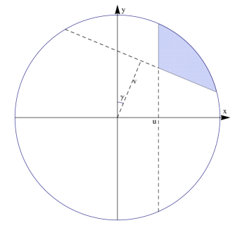
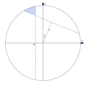
Let ( X , Y ) ∼ f ( x , y ) similar-to 𝑋 𝑌 𝑓 𝑥 𝑦 (X,Y)\sim f(x,y) 3.4 B 2 subscript 𝐵 2 B_{2} [ − 1 , 1 ] 1 1 [-1,1] γ ∈ ( − π / 2 , π / 2 ) 𝛾 𝜋 2 𝜋 2 \gamma\in(-\pi/2,\pi/2)
U = X , V γ = X sin γ + Y cos γ . formulae-sequence 𝑈 𝑋 subscript 𝑉 𝛾 𝑋 𝛾 𝑌 𝛾 U=X,\quad V_{\gamma}=X\sin\gamma+Y\cos\gamma. (5.1)
By the circular symmetry of ( X , Y ) 𝑋 𝑌 (X,Y) V γ = d Y ∼ uniform [ − 1 , 1 ] superscript 𝑑 subscript 𝑉 𝛾 𝑌 similar-to uniform 1 1 V_{\gamma}\buildrel d\over{=}Y\sim\mathrm{uniform}[-1,1] ( U , V γ ) 𝑈 subscript 𝑉 𝛾 (U,V_{\gamma}) C 2 subscript 𝐶 2 C_{2} ( U , V γ ) 𝑈 subscript 𝑉 𝛾 (U,V_{\gamma}) f γ ( u , v ) subscript 𝑓 𝛾 𝑢 𝑣 f_{\gamma}(u,v) F γ ( u , v ) subscript 𝐹 𝛾 𝑢 𝑣 F_{\gamma}(u,v) { F γ ∣ γ ∈ ( − π / 2 , π / 2 ) } conditional-set subscript 𝐹 𝛾 𝛾 𝜋 2 𝜋 2 \{F_{\gamma}\mid\gamma\in(-\pi/2,\pi/2)\} elliptical copulas , so-called because the support of ( U , V γ ) 𝑈 subscript 𝑉 𝛾 (U,V_{\gamma})
E γ := { ( u , v ) ∣ u 2 + v 2 − 2 u v sin γ ≤ cos 2 γ } . assign subscript 𝐸 𝛾 conditional-set 𝑢 𝑣 superscript 𝑢 2 superscript 𝑣 2 2 𝑢 𝑣 𝛾 superscript 2 𝛾 E_{\gamma}:=\{(u,v)\mid u^{2}+v^{2}-2uv\sin\gamma\leq\cos^{2}\gamma\}. (5.2)
(Note that E 0 = B 2 subscript 𝐸 0 subscript 𝐵 2 E_{0}=B_{2} 5.1 U 𝑈 U V γ subscript 𝑉 𝛾 V_{\gamma}
ρ ( U , V γ ) = sin γ , 𝜌 𝑈 subscript 𝑉 𝛾 𝛾 \rho(U,V_{\gamma})=\sin\gamma, (5.3)
so γ 𝛾 \gamma U 𝑈 U V γ subscript 𝑉 𝛾 V_{\gamma}
Proposition 5.1 .
The pdf of ( U , V γ ) 𝑈 subscript 𝑉 𝛾 (U,V_{\gamma})
f γ ( u , v ) = 1 2 π cos 2 γ − u 2 − v 2 + 2 u v sin γ 1 E γ ( u , v ) . subscript 𝑓 𝛾 𝑢 𝑣 1 2 𝜋 superscript 2 𝛾 superscript 𝑢 2 superscript 𝑣 2 2 𝑢 𝑣 𝛾 subscript 1 subscript 𝐸 𝛾 𝑢 𝑣 f_{\gamma}(u,v)=\frac{1}{2\pi\sqrt{\cos^{2}\gamma-u^{2}-v^{2}+2uv\sin\gamma}}1_{E_{\gamma}}(u,v). (5.4)
Proof.
The pdf can be obtained by a standard Jacobian computation. From (5.1
x ( u , v ) = u , y ( u , v ) = v − u sin γ cos ( γ ) , formulae-sequence 𝑥 𝑢 𝑣 𝑢 𝑦 𝑢 𝑣 𝑣 𝑢 𝛾 𝛾 x(u,v)=u,\quad y(u,v)=\frac{v-u\sin\gamma}{\cos(\gamma)}, (5.5)
so
∂ x ( u , v ) ∂ u = 1 , ∂ x ( u , v ) ∂ v = 0 , ∂ y ( u , v ) ∂ u = − tan γ , ∂ y ( u , v ) ∂ v = 1 cos γ . 𝑥 𝑢 𝑣 𝑢 1 𝑥 𝑢 𝑣 𝑣 0 𝑦 𝑢 𝑣 𝑢 𝛾 𝑦 𝑢 𝑣 𝑣 1 𝛾 \displaystyle\begin{array}[]{l l}\frac{\partial x(u,v)}{\partial u}=1,&\frac{\partial x(u,v)}{\partial v}=0,\\
\frac{\partial y(u,v)}{\partial u}=-\tan\gamma,&\frac{\partial y(u,v)}{\partial v}=\frac{1}{\cos\gamma}.\end{array}
Thus the Jacobian of the transformation is J = 1 / cos γ 𝐽 1 𝛾 J=1/\cos\gamma 3.4
f γ ( u , v ) subscript 𝑓 𝛾 𝑢 𝑣 \displaystyle f_{\gamma}(u,v) = \displaystyle= f ( x ( u , v ) , y ( u , v ) ) ⋅ J ⋅ 𝑓 𝑥 𝑢 𝑣 𝑦 𝑢 𝑣 𝐽 \displaystyle f(x(u,v),y(u,v))\cdot J
= \displaystyle= 1 2 π 1 − u 2 − ( v − u sin γ ) 2 / cos 2 γ 1 B 2 ( x ( u , v ) , y ( u , v ) ) ⋅ 1 cos γ ⋅ 1 2 𝜋 1 superscript 𝑢 2 superscript 𝑣 𝑢 𝛾 2 superscript 2 𝛾 subscript 1 subscript 𝐵 2 𝑥 𝑢 𝑣 𝑦 𝑢 𝑣 1 𝛾 \displaystyle\frac{1}{2\pi\sqrt{1-u^{2}-(v-u\sin\gamma)^{2}/\cos^{2}\gamma}}1_{B_{2}}(x(u,v),y(u,v))\cdot\frac{1}{\cos\gamma}
= \displaystyle= cos γ 2 π ( 1 − u 2 ) cos 2 γ − ( v − u sin γ ) 2 1 cos γ ⋅ 1 B 2 ( x ( u , v ) , y ( u , v ) ) ⋅ 𝛾 2 𝜋 1 superscript 𝑢 2 superscript 2 𝛾 superscript 𝑣 𝑢 𝛾 2 1 𝛾 subscript 1 subscript 𝐵 2 𝑥 𝑢 𝑣 𝑦 𝑢 𝑣 \displaystyle\frac{\cos\gamma}{2\pi\sqrt{(1-u^{2})\cos^{2}\gamma-(v-u\sin\gamma)^{2}}}\frac{1}{\cos\gamma}\cdot 1_{B_{2}}(x(u,v),y(u,v))
= \displaystyle= 1 2 π cos 2 γ − u 2 − v 2 + 2 u v sin γ 1 E γ ( u , v ) . 1 2 𝜋 superscript 2 𝛾 superscript 𝑢 2 superscript 𝑣 2 2 𝑢 𝑣 𝛾 subscript 1 subscript 𝐸 𝛾 𝑢 𝑣 \displaystyle\frac{1}{2\pi\sqrt{\cos^{2}\gamma-u^{2}-v^{2}+2uv\sin\gamma}}1_{E_{\gamma}}(u,v).
∎
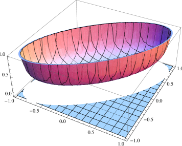
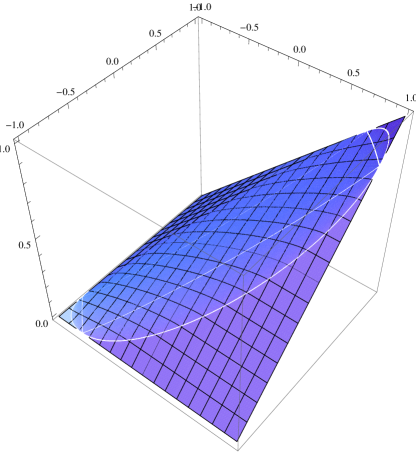
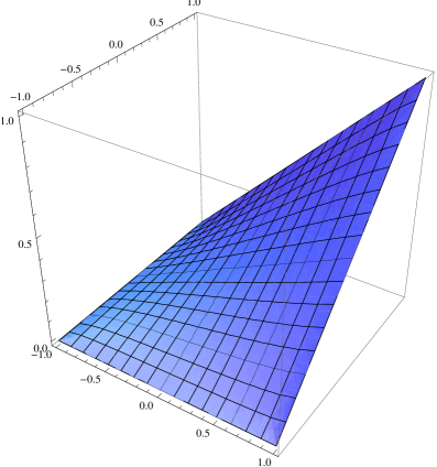
Figure 8 f γ ( u , v ) subscript 𝑓 𝛾 𝑢 𝑣 f_{\gamma}(u,v) γ = π / 4 𝛾 𝜋 4 \gamma=\pi/4
Figure 8. The density f γ ( u , v ) subscript 𝑓 𝛾 𝑢 𝑣 f_{\gamma}(u,v) γ = π / 4 𝛾 𝜋 4 \gamma=\pi/4
To describe the family of elliptical copulas F γ subscript 𝐹 𝛾 F_{\gamma} 3.14 3.16 ( u , v ) ∈ E γ 𝑢 𝑣 subscript 𝐸 𝛾 (u,v)\in E_{\gamma}
α γ ( u , v ) subscript 𝛼 𝛾 𝑢 𝑣 \displaystyle\alpha_{\gamma}(u,v) = \displaystyle= 1 2 π [ u arcsin ( v − u sin γ cos γ 1 − u 2 ) + v arcsin ( u − v sin γ cos γ 1 − v 2 ) \displaystyle\frac{1}{2\pi}\left[u\arcsin\left(\frac{v-u\sin\gamma}{\cos\gamma\sqrt{1-u^{2}}}\right)+v\arcsin\left(\frac{u-v\sin\gamma}{\cos\gamma\sqrt{1-v^{2}}}\right)\right. (5.7)
− arcsin ( u v − sin γ ( 1 − u 2 ) ( 1 − v 2 ) ) ] . \displaystyle\left.\qquad-\arcsin\left(\frac{uv-\sin\gamma}{\sqrt{(1-u^{2})(1-v^{2})}}\right)\right].
Note that α γ subscript 𝛼 𝛾 \alpha_{\gamma} α 𝛼 \alpha 3.14 γ = 0 𝛾 0 \gamma=0 V γ = Y subscript 𝑉 𝛾 𝑌 V_{\gamma}=Y 3.10
A ( arccos u , arccos v ; π 2 − γ ) = ( 1 − u − v ) π + 4 π α γ ( u , v ) . 𝐴 𝑢 𝑣 𝜋 2 𝛾 1 𝑢 𝑣 𝜋 4 𝜋 subscript 𝛼 𝛾 𝑢 𝑣 A(\arccos u,\,\arccos v;\,\frac{\pi}{2}-\gamma)=(1-u-v)\pi+4\pi\alpha_{\gamma}(u,v). (5.8)
Next, extend the definition of α γ ( u , v ) subscript 𝛼 𝛾 𝑢 𝑣 \alpha_{\gamma}(u,v) C 2 ∖ E γ subscript 𝐶 2 subscript 𝐸 𝛾 C_{2}\setminus E_{\gamma} 9
α γ ( u , v ) = { u + v − 1 4 if ( u , v ) ∈ R 5 ( γ ) := ( C 2 ∖ E γ ) ∩ { ( u , v ) ∣ u + v > 1 + sin γ } , u − v + 1 4 if ( u , v ) ∈ R 6 ( γ ) := ( C 2 ∖ E γ ) ∩ { ( u , v ) ∣ v − u > 1 − sin γ } , − u + v + 1 4 if ( u , v ) ∈ R 7 ( γ ) := ( C 2 ∖ E γ ) ∩ { ( u , v ) ∣ v − u < sin γ − 1 } , − u − v − 1 4 if ( u , v ) ∈ R 8 ( γ ) := ( C 2 ∖ E γ ) ∩ { ( u , v ) ∣ u + v < − sin γ − 1 } . subscript 𝛼 𝛾 𝑢 𝑣 cases 𝑢 𝑣 1 4 if 𝑢 𝑣 subscript 𝑅 5 𝛾 assign subscript 𝐶 2 subscript 𝐸 𝛾 conditional-set 𝑢 𝑣 𝑢 𝑣 1 𝛾 𝑢 𝑣 1 4 if 𝑢 𝑣 subscript 𝑅 6 𝛾 assign subscript 𝐶 2 subscript 𝐸 𝛾 conditional-set 𝑢 𝑣 𝑣 𝑢 1 𝛾 𝑢 𝑣 1 4 if 𝑢 𝑣 subscript 𝑅 7 𝛾 assign subscript 𝐶 2 subscript 𝐸 𝛾 conditional-set 𝑢 𝑣 𝑣 𝑢 𝛾 1 𝑢 𝑣 1 4 if 𝑢 𝑣 subscript 𝑅 8 𝛾 assign subscript 𝐶 2 subscript 𝐸 𝛾 conditional-set 𝑢 𝑣 𝑢 𝑣 𝛾 1 \alpha_{\gamma}(u,v)=\begin{cases}\frac{u+v-1}{4}&\mathrm{if}\ (u,v)\in R_{5}(\gamma):=(C_{2}\setminus E_{\gamma})\cap\{(u,v)\mid u+v>1+\sin\gamma\},\\
\frac{u-v+1}{4}&\mathrm{if}\ (u,v)\in R_{6}(\gamma):=(C_{2}\setminus E_{\gamma})\cap\{(u,v)\mid v-u>1-\sin\gamma\},\\
\frac{-u+v+1}{4}&\mathrm{if}\ (u,v)\in R_{7}(\gamma):=(C_{2}\setminus E_{\gamma})\cap\{(u,v)\mid v-u<\sin\gamma-1\},\\
\frac{-u-v-1}{4}&\mathrm{if}\ (u,v)\in R_{8}(\gamma):=(C_{2}\setminus E_{\gamma})\cap\{(u,v)\mid u+v<-\sin\gamma-1\}.\end{cases} (5.9)
Note that (5.7 5.9 ∂ E γ subscript 𝐸 𝛾 \partial E_{\gamma} u 2 + v 2 − 2 u v sin γ = cos 2 γ superscript 𝑢 2 superscript 𝑣 2 2 𝑢 𝑣 𝛾 superscript 2 𝛾 u^{2}+v^{2}-2uv\sin\gamma=\cos^{2}\gamma 5.9 α 𝛼 \alpha 3.16 γ = 0 𝛾 0 \gamma=0 5.3
Lemma 5.2 .
Let ( U , V ) 𝑈 𝑉 (U,V) C 2 subscript 𝐶 2 C_{2} [ − 1 , 1 ] 1 1 [-1,1] ( U , V ) = d ( − U , − V ) superscript 𝑑 𝑈 𝑉 𝑈 𝑉 (U,V)\buildrel d\over{=}(-U,-V) F ( u , v ) 𝐹 𝑢 𝑣 F(u,v)
F ( u , v ) = u + v 2 + F ( − u , − v ) , ( u , v ) ∈ C 2 . formulae-sequence 𝐹 𝑢 𝑣 𝑢 𝑣 2 𝐹 𝑢 𝑣 𝑢 𝑣 subscript 𝐶 2 F(u,v)=\frac{u+v}{2}+F(-u,-v),\quad(u,v)\in C_{2}. (5.10)
Proof.
By the symmetry condition,
F ( u , v ) 𝐹 𝑢 𝑣 \displaystyle F(u,v) = \displaystyle= P [ − U ≤ u , − V ≤ v ] = P [ U ≥ − u , V ≥ − v ] 𝑃 delimited-[] formulae-sequence 𝑈 𝑢 𝑉 𝑣 𝑃 delimited-[] formulae-sequence 𝑈 𝑢 𝑉 𝑣 \displaystyle P[-U\leq u,\,-V\leq v]=P[U\geq-u,\,V\geq-v]
= \displaystyle= 1 − P [ U < − u ] − P [ V < − v ] + P [ U < − u , V < − v ] 1 𝑃 delimited-[] 𝑈 𝑢 𝑃 delimited-[] 𝑉 𝑣 𝑃 delimited-[] formulae-sequence 𝑈 𝑢 𝑉 𝑣 \displaystyle 1-P[U<-u]-P[V<-v]+P[U<-u,\,V<-v]
= \displaystyle= 1 − ( − u + 1 2 ) + ( − v + 1 2 ) + P [ U ≤ − u , V ≤ − v ] 1 𝑢 1 2 𝑣 1 2 𝑃 delimited-[] formulae-sequence 𝑈 𝑢 𝑉 𝑣 \displaystyle 1-\left(\frac{-u+1}{2}\right)+\left(\frac{-v+1}{2}\right)+P[U\leq-u,\,V\leq-v]
= \displaystyle= u + v 2 + F ( − u , − v ) . 𝑢 𝑣 2 𝐹 𝑢 𝑣 \displaystyle\frac{u+v}{2}+F(-u,\,-v).
∎
Figure 9. Eight regions R 1 ( γ ) − R 8 ( γ ) subscript 𝑅 1 𝛾 subscript 𝑅 8 𝛾 R_{1}(\gamma)-R_{8}(\gamma) γ = π / 8 𝛾 𝜋 8 \gamma=\pi/8
Theorem 5.3 .
The cdf ≡ \equiv ( U , V γ ) 𝑈 subscript 𝑉 𝛾 (U,V_{\gamma})
F γ ( u , v ) = u + v + 1 4 + α γ ( u , v ) , ( u , v ) ∈ C 2 . formulae-sequence subscript 𝐹 𝛾 𝑢 𝑣 𝑢 𝑣 1 4 subscript 𝛼 𝛾 𝑢 𝑣 𝑢 𝑣 subscript 𝐶 2 F_{\gamma}(u,v)=\frac{u+v+1}{4}+\alpha_{\gamma}(u,v),\qquad\qquad(u,v)\in C_{2}. (5.11)
Proof.
To find F γ ( u , v ) subscript 𝐹 𝛾 𝑢 𝑣 F_{\gamma}(u,v) 3.10 ∂ B 3 subscript 𝐵 3 \partial B_{3} 3 5.11 C 2 = ∪ i = 1 8 R i ( γ ) subscript 𝐶 2 superscript subscript 𝑖 1 8 subscript 𝑅 𝑖 𝛾 C_{2}=\cup_{i=1}^{8}R_{i}(\gamma) R 5 ( γ ) − R 8 ( γ ) subscript 𝑅 5 𝛾 subscript 𝑅 8 𝛾 R_{5}(\gamma)-R_{8}(\gamma) 5.9 9
R 1 ( γ ) subscript 𝑅 1 𝛾 \displaystyle R_{1}(\gamma) = \displaystyle= E γ ∩ { ( u , v ) ∣ 0 ≤ u , v ≤ 1 } , subscript 𝐸 𝛾 conditional-set 𝑢 𝑣 formulae-sequence 0 𝑢 𝑣 1 \displaystyle E_{\gamma}\cap\{(u,v)\mid 0\leq u,v\leq 1\},
R 2 ( γ ) subscript 𝑅 2 𝛾 \displaystyle R_{2}(\gamma) = \displaystyle= E γ ∩ { ( u , v ) ∣ − 1 ≤ u ≤ 0 ≤ v ≤ 1 } , subscript 𝐸 𝛾 conditional-set 𝑢 𝑣 1 𝑢 0 𝑣 1 \displaystyle E_{\gamma}\cap\{(u,v)\mid-1\leq u\leq 0\leq v\leq 1\},
R 3 ( γ ) subscript 𝑅 3 𝛾 \displaystyle R_{3}(\gamma) = \displaystyle= E γ ∩ { ( u , v ) ∣ − 1 ≤ v ≤ 0 ≤ u ≤ 1 } , subscript 𝐸 𝛾 conditional-set 𝑢 𝑣 1 𝑣 0 𝑢 1 \displaystyle E_{\gamma}\cap\{(u,v)\mid-1\leq v\leq 0\leq u\leq 1\},
R 4 ( γ ) subscript 𝑅 4 𝛾 \displaystyle R_{4}(\gamma) = \displaystyle= E γ ∩ { ( u , v ) ∣ − 1 ≤ u , v ≤ 0 } . subscript 𝐸 𝛾 conditional-set 𝑢 𝑣 formulae-sequence 1 𝑢 𝑣 0 \displaystyle E_{\gamma}\cap\{(u,v)\mid-1\leq u,v\leq 0\}.
Case 1: ( u , v ) ∈ R 1 ( γ ) 𝑢 𝑣 subscript 𝑅 1 𝛾 (u,v)\in R_{1}(\gamma) 10
Figure 10. The region [ X > u , X sin ( γ ) + Y cos ( γ ) > v ] delimited-[] formulae-sequence 𝑋 𝑢 𝑋 𝛾 𝑌 𝛾 𝑣 [X>u,X\sin(\gamma)+Y\cos(\gamma)>v] γ = π / 8 𝛾 𝜋 8 \gamma=\pi/8
F γ ( u , v ) subscript 𝐹 𝛾 𝑢 𝑣 \displaystyle F_{\gamma}(u,v) = \displaystyle= P [ U ≤ u , V γ ≤ v ] 𝑃 delimited-[] formulae-sequence 𝑈 𝑢 subscript 𝑉 𝛾 𝑣 \displaystyle P[U\leq u,\,V_{\gamma}\leq v]
= \displaystyle= 1 − P [ U > u ] − P [ V γ > v ] + P [ U > u , V γ > v ] 1 𝑃 delimited-[] 𝑈 𝑢 𝑃 delimited-[] subscript 𝑉 𝛾 𝑣 𝑃 delimited-[] formulae-sequence 𝑈 𝑢 subscript 𝑉 𝛾 𝑣 \displaystyle 1-P[U>u]-P[V_{\gamma}>v]+P[U>u,\,V_{\gamma}>v]
= \displaystyle= 1 − ( 1 − u 2 ) − ( 1 − v 2 ) + P [ X > u , X sin γ + Y cos γ > v ] 1 1 𝑢 2 1 𝑣 2 𝑃 delimited-[] formulae-sequence 𝑋 𝑢 𝑋 𝛾 𝑌 𝛾 𝑣 \displaystyle 1-\left(\frac{1-u}{2}\right)-\left(\frac{1-v}{2}\right)+P[X>u,\,X\sin\gamma+Y\cos\gamma>v]
= \displaystyle= u + v 2 + 1 4 π A ( arccos u , arccos v ; π / 2 − γ ) 𝑢 𝑣 2 1 4 𝜋 𝐴 𝑢 𝑣 𝜋 2 𝛾 \displaystyle\frac{u+v}{2}+\frac{1}{4\pi}A(\arccos u,\arccos v;\,\pi/2-\gamma)
= \displaystyle= u + v + 1 4 + α γ ( u , v ) [ by ( 5.8 ) ] . 𝑢 𝑣 1 4 subscript 𝛼 𝛾 𝑢 𝑣 delimited-[] by ( 5.8 )
\displaystyle\frac{u+v+1}{4}+\alpha_{\gamma}(u,v)\qquad\qquad\qquad\qquad\qquad\mathrm{[by\ \eqref{Apsigamma}]}.
Case 2: ( u , v ) ) ∈ R 2 ( γ ) (u,v))\in R_{2}(\gamma) ( X , Y ) = d ( − X , Y ) superscript 𝑑 𝑋 𝑌 𝑋 𝑌 (X,Y)\buildrel d\over{=}(-X,Y) 11
F γ ( u , v ) subscript 𝐹 𝛾 𝑢 𝑣 \displaystyle F_{\gamma}(u,v) = \displaystyle= P [ U ≤ u ] − P [ U ≤ u , V γ > v ] 𝑃 delimited-[] 𝑈 𝑢 𝑃 delimited-[] formulae-sequence 𝑈 𝑢 subscript 𝑉 𝛾 𝑣 \displaystyle P[U\leq u]-P[U\leq u,\,V_{\gamma}>v]
= \displaystyle= u + 1 2 − P [ X ≤ u , X sin γ + Y cos γ > v ] 𝑢 1 2 𝑃 delimited-[] formulae-sequence 𝑋 𝑢 𝑋 𝛾 𝑌 𝛾 𝑣 \displaystyle\frac{u+1}{2}-P[X\leq u,\,X\sin\gamma+Y\cos\gamma>v]
= \displaystyle= u + 1 2 − P [ − X ≤ u , − X sin γ + Y cos γ > v ] 𝑢 1 2 𝑃 delimited-[] formulae-sequence 𝑋 𝑢 𝑋 𝛾 𝑌 𝛾 𝑣 \displaystyle\frac{u+1}{2}-P[-X\leq u,\,-X\sin\gamma+Y\cos\gamma>v]
= \displaystyle= u + 1 2 − P [ X ≥ − u , X sin ( − γ ) + Y cos ( − γ ) > v ] 𝑢 1 2 𝑃 delimited-[] formulae-sequence 𝑋 𝑢 𝑋 𝛾 𝑌 𝛾 𝑣 \displaystyle\frac{u+1}{2}-P[X\geq-u,\,X\sin(-\gamma)+Y\cos(-\gamma)>v]
= \displaystyle= u + 1 2 − 1 4 π A ( arccos ( − u ) , arccos v ; π / 2 + γ ) 𝑢 1 2 1 4 𝜋 𝐴 𝑢 𝑣 𝜋 2 𝛾 \displaystyle\frac{u+1}{2}-\frac{1}{4\pi}A(\arccos(-u),\arccos v;\,\pi/2+\gamma)
= \displaystyle= u + v + 1 4 − α − γ ( − u , v ) [ by ( 5.8 ) ] 𝑢 𝑣 1 4 subscript 𝛼 𝛾 𝑢 𝑣 delimited-[] by ( 5.8 )
\displaystyle\frac{u+v+1}{4}-\alpha_{-\gamma}(-u,v)\ \ \qquad\qquad\qquad\qquad\mathrm{[by\ \eqref{Apsigamma}]}
= \displaystyle= u + v + 1 4 + α γ ( u , v ) [ by ( 5.7 ) ] . 𝑢 𝑣 1 4 subscript 𝛼 𝛾 𝑢 𝑣 delimited-[] by ( 5.7 )
\displaystyle\frac{u+v+1}{4}+\alpha_{\gamma}(u,v)\qquad\qquad\qquad\qquad\qquad\mathrm{[by\ \eqref{psigamma}]}.
Figure 11. The region [ X < u , X sin ( γ ) + Y cos ( γ ) > v ] delimited-[] formulae-sequence 𝑋 𝑢 𝑋 𝛾 𝑌 𝛾 𝑣 [X<u,X\sin(\gamma)+Y\cos(\gamma)>v] γ = π / 8 𝛾 𝜋 8 \gamma=\pi/8
Case 3: ( u , v ) ∈ R 3 ( γ ) 𝑢 𝑣 subscript 𝑅 3 𝛾 (u,v)\in R_{3}(\gamma) ( − u , − v ) ∈ R 2 ( γ ) 𝑢 𝑣 subscript 𝑅 2 𝛾 (-u,-v)\in R_{2}(\gamma) 5.2
F γ ( u , v ) subscript 𝐹 𝛾 𝑢 𝑣 \displaystyle F_{\gamma}(u,v) = \displaystyle= u + v 2 + F γ ( − u , − v ) 𝑢 𝑣 2 subscript 𝐹 𝛾 𝑢 𝑣 \displaystyle\frac{u+v}{2}+F_{\gamma}(-u,-v)
= \displaystyle= u + v 2 + − u − v + 1 4 + α γ ( − u , − v ) 𝑢 𝑣 2 𝑢 𝑣 1 4 subscript 𝛼 𝛾 𝑢 𝑣 \displaystyle\frac{u+v}{2}+\frac{-u-v+1}{4}+\alpha_{\gamma}(-u,-v)
= \displaystyle= u + v + 1 4 + α γ ( u , v ) [ by ( 5.7 ) ] . 𝑢 𝑣 1 4 subscript 𝛼 𝛾 𝑢 𝑣 delimited-[] by ( 5.7 )
\displaystyle\frac{u+v+1}{4}+\alpha_{\gamma}(u,v)\qquad\qquad\qquad\qquad\mathrm{[by\ \eqref{psigamma}]}.
Case 4: ( u , v ) ∈ R 4 ( γ ) 𝑢 𝑣 subscript 𝑅 4 𝛾 (u,v)\in R_{4}(\gamma) ( − u , − v ) ∈ R 1 ( γ ) 𝑢 𝑣 subscript 𝑅 1 𝛾 (-u,-v)\in R_{1}(\gamma) 5.2
Case 5: ( u , v ) ∈ R 5 ( γ ) 𝑢 𝑣 subscript 𝑅 5 𝛾 (u,v)\in R_{5}(\gamma)
F γ ( u , v ) subscript 𝐹 𝛾 𝑢 𝑣 \displaystyle F_{\gamma}(u,v) = \displaystyle= 1 − P [ U > u ] − P [ V γ > v ] 1 𝑃 delimited-[] 𝑈 𝑢 𝑃 delimited-[] subscript 𝑉 𝛾 𝑣 \displaystyle 1-P[U>u]-P[V_{\gamma}>v]
= \displaystyle= 1 − ( 1 − u 2 ) − ( 1 − v 2 ) 1 1 𝑢 2 1 𝑣 2 \displaystyle 1-\left(\frac{1-u}{2}\right)-\left(\frac{1-v}{2}\right)
= \displaystyle= u + v + 1 4 + α γ ( u , v ) [ by ( 5.9 ) ] . 𝑢 𝑣 1 4 subscript 𝛼 𝛾 𝑢 𝑣 delimited-[] by ( 5.9 )
\displaystyle\frac{u+v+1}{4}+\alpha_{\gamma}(u,v)\qquad\qquad\qquad[\mathrm{by\ \eqref{psigammaextension}}].
Case 6: ( u , v ) ∈ R 6 ( γ ) 𝑢 𝑣 subscript 𝑅 6 𝛾 (u,v)\in R_{6}(\gamma)
F γ ( u , v ) subscript 𝐹 𝛾 𝑢 𝑣 \displaystyle F_{\gamma}(u,v) = \displaystyle= P [ U ≤ u ] 𝑃 delimited-[] 𝑈 𝑢 \displaystyle P[U\leq u]
= \displaystyle= u + 1 2 𝑢 1 2 \displaystyle\frac{u+1}{2}
= \displaystyle= u + v + 1 4 + α γ ( u , v ) [ by ( 5.9 ) ] . 𝑢 𝑣 1 4 subscript 𝛼 𝛾 𝑢 𝑣 delimited-[] by ( 5.9 )
\displaystyle\frac{u+v+1}{4}+\alpha_{\gamma}(u,v)\qquad\qquad\qquad[\mathrm{by\ \eqref{psigammaextension}}].
Case 7: ( u , v ) ∈ R 7 ( γ ) 𝑢 𝑣 subscript 𝑅 7 𝛾 (u,v)\in R_{7}(\gamma) ( − u , − v ) ∈ R 6 ( γ ) 𝑢 𝑣 subscript 𝑅 6 𝛾 (-u,-v)\in R_{6}(\gamma) 5.2
Case 8: ( u , v ) ∈ R 8 ( γ ) 𝑢 𝑣 subscript 𝑅 8 𝛾 (u,v)\in R_{8}(\gamma) ( − u , − v ) ∈ R 5 ( γ ) 𝑢 𝑣 subscript 𝑅 5 𝛾 (-u,-v)\in R_{5}(\gamma) 5.2
Figure 12. The copula F γ ( u , v ) subscript 𝐹 𝛾 𝑢 𝑣 F_{\gamma}(u,v) γ = π / 4 𝛾 𝜋 4 \gamma=\pi/4
6. Copulas Derived from the Uniform Distribution on the Unit Ball
Up to now we have addressed the question of whether copulas can be
generated by means of linear functions of a circularly symmetric or
spherically symmetric random vector. Now we ask whether non-linear
functions of such random vectors can generate copulas.
We shall restrict attention to random vectors uniformly distributed
over the unit ball B d subscript 𝐵 𝑑 B_{d} C d subscript 𝐶 𝑑 C_{d}
We begin with the bivariate case. Suppose that ( X , Y ) 𝑋 𝑌 (X,Y) B 2 = { ( x , y ) ∈ ℝ 2 ∣ x 2 + y 2 ≤ 1 } subscript 𝐵 2 conditional-set 𝑥 𝑦 superscript ℝ 2 superscript 𝑥 2 superscript 𝑦 2 1 B_{2}=\{(x,y)\in\mathbb{R}^{2}\mid\ x^{2}+y^{2}\leq 1\}
X ∣ Y conditional 𝑋 𝑌 \displaystyle X\mid Y ∼ similar-to \displaystyle\sim uniform [ − 1 − Y 2 , 1 − Y 2 ] uniform 1 superscript 𝑌 2 1 superscript 𝑌 2 \displaystyle\mathrm{uniform}[-\sqrt{1-Y^{2}},\,\sqrt{1-Y^{2}}]
and Y ∣ X and conditional 𝑌 𝑋
\displaystyle\mathrm{and}\qquad Y\mid X ∼ similar-to \displaystyle\sim uniform [ − 1 − X 2 , 1 − X 2 ] , uniform 1 superscript 𝑋 2 1 superscript 𝑋 2 \displaystyle\mathrm{uniform}[-\sqrt{1-X^{2}},\,\sqrt{1-X^{2}}],
it follows that the random variables
U := X 1 − Y 2 , V := Y 1 − X 2 formulae-sequence assign 𝑈 𝑋 1 superscript 𝑌 2 assign 𝑉 𝑌 1 superscript 𝑋 2 U:=\frac{X}{\sqrt{1-Y^{2}}},\qquad V:=\frac{Y}{\sqrt{1-X^{2}}} (6.1)
satisfy
U ∣ Y conditional 𝑈 𝑌 \displaystyle U\mid Y ∼ similar-to \displaystyle\sim uniform [ − 1 , 1 ] uniform 1 1 \displaystyle\mathrm{uniform}[-1,1]
V ∣ X conditional 𝑉 𝑋 \displaystyle V\mid X ∼ similar-to \displaystyle\sim uniform [ − 1 , 1 ] . uniform 1 1 \displaystyle\mathrm{uniform}[-1,1].
Thus, U 𝑈 U Y 𝑌 Y V 𝑉 V X 𝑋 X
U 𝑈 \displaystyle U ∼ similar-to \displaystyle\sim uniform [ − 1 , 1 ] uniform 1 1 \displaystyle\mathrm{uniform}[-1,1]
V 𝑉 \displaystyle\qquad V ∼ similar-to \displaystyle\sim uniform [ − 1 , 1 ] , uniform 1 1 \displaystyle\mathrm{uniform}[-1,1],
so the joint distribution of ( U , V ) 𝑈 𝑉 (U,V) F ( u , v ) F_{(}u,v) C 2 ≡ [ − 1 , 1 ] 2 subscript 𝐶 2 superscript 1 1 2 C_{2}\equiv[-1,1]^{2} U 𝑈 U V 𝑉 V ( X , Y ) 𝑋 𝑌 (X,Y)
Question 6:
Are U 𝑈 U V 𝑉 V
Answer 6. Clearly U 𝑈 U V 𝑉 V E ( U ) = E ( V ) = 0 𝐸 𝑈 𝐸 𝑉 0 E(U)=E(V)=0
E ( U V ) = E ( X Y ( 1 − X 2 ) ( 1 − Y 2 ) ) = 0 , 𝐸 𝑈 𝑉 𝐸 𝑋 𝑌 1 superscript 𝑋 2 1 superscript 𝑌 2 0 E(UV)=E\left(\frac{XY}{\sqrt{(1-X^{2})(1-Y^{2})}}\right)=0,
all by the circular symmetry of ( X , Y ) 𝑋 𝑌 (X,Y) ( U , V ) 𝑈 𝑉 (U,V)
Proposition 6.1 .
The joint density of ( U , V ) 𝑈 𝑉 (U,V)
f ( u , v ) = 1 π ( 1 − u 2 ) ( 1 − v 2 ) ( 1 − u 2 v 2 ) 2 1 C 2 ( u , v ) . 𝑓 𝑢 𝑣 1 𝜋 1 superscript 𝑢 2 1 superscript 𝑣 2 superscript 1 superscript 𝑢 2 superscript 𝑣 2 2 subscript 1 subscript 𝐶 2 𝑢 𝑣 \displaystyle f(u,v)=\frac{1}{\pi}\frac{\sqrt{(1-u^{2})(1-v^{2})}}{(1-u^{2}v^{2})^{2}}1_{C_{2}}(u,v). (6.2)
Figure 13. Joint density f ( u , v ) 𝑓 𝑢 𝑣 f(u,v) ( U , V ) 𝑈 𝑉 (U,V)
Proof.
This pdf is again obtained via the Jacobian method. It follows from (6.1
u 2 ( 1 − y 2 ) = x 2 , and v 2 ( 1 − x 2 ) = y 2 . formulae-sequence superscript 𝑢 2 1 superscript 𝑦 2 superscript 𝑥 2 and
superscript 𝑣 2 1 superscript 𝑥 2 superscript 𝑦 2 \displaystyle u^{2}(1-y^{2})=x^{2},\qquad\mbox{and}\qquad v^{2}(1-x^{2})=y^{2}.
Substitution of the second expression for y 2 superscript 𝑦 2 y^{2}
x 2 = u 2 ( 1 − v 2 ) 1 − u 2 v 2 , y 2 = v 2 ( 1 − u 2 ) 1 − u 2 v 2 , formulae-sequence superscript 𝑥 2 superscript 𝑢 2 1 superscript 𝑣 2 1 superscript 𝑢 2 superscript 𝑣 2 superscript 𝑦 2 superscript 𝑣 2 1 superscript 𝑢 2 1 superscript 𝑢 2 superscript 𝑣 2 \displaystyle x^{2}=\frac{u^{2}(1-v^{2})}{1-u^{2}v^{2}},\qquad y^{2}=\frac{v^{2}(1-u^{2})}{1-u^{2}v^{2}},
so, since x 𝑥 x u 𝑢 u y 𝑦 y v 𝑣 v 6.1
x ≡ x ( u , v ) = u 1 − v 2 1 − u 2 v 2 , y ≡ y ( u , v ) = v 1 − u 2 1 − u 2 v 2 . formulae-sequence 𝑥 𝑥 𝑢 𝑣 𝑢 1 superscript 𝑣 2 1 superscript 𝑢 2 superscript 𝑣 2 𝑦 𝑦 𝑢 𝑣 𝑣 1 superscript 𝑢 2 1 superscript 𝑢 2 superscript 𝑣 2 x\equiv x(u,v)=\frac{u\sqrt{1-v^{2}}}{\sqrt{1-u^{2}v^{2}}},\qquad y\equiv y(u,v)=\frac{v\sqrt{1-u^{2}}}{\sqrt{1-u^{2}v^{2}}}. (6.3)
Thus
∂ x ∂ u 𝑥 𝑢 \displaystyle\frac{\partial x}{\partial u} = \displaystyle= 1 − v 2 [ 1 1 − u 2 v 2 + u ( 1 − u 2 v 2 ) − 3 / 2 ( u v 2 ) ] 1 superscript 𝑣 2 delimited-[] 1 1 superscript 𝑢 2 superscript 𝑣 2 𝑢 superscript 1 superscript 𝑢 2 superscript 𝑣 2 3 2 𝑢 superscript 𝑣 2 \displaystyle\sqrt{1-v^{2}}\left[\frac{1}{\sqrt{1-u^{2}v^{2}}}+u(1-u^{2}v^{2})^{-3/2}(uv^{2})\right]
= \displaystyle= 1 − v 2 1 − u 2 v 2 { 1 + u 2 v 2 1 − u 2 v 2 } 1 superscript 𝑣 2 1 superscript 𝑢 2 superscript 𝑣 2 1 superscript 𝑢 2 superscript 𝑣 2 1 superscript 𝑢 2 superscript 𝑣 2 \displaystyle\frac{\sqrt{1-v^{2}}}{\sqrt{1-u^{2}v^{2}}}\left\{1+\frac{u^{2}v^{2}}{1-u^{2}v^{2}}\right\}
= \displaystyle= 1 − v 2 ( 1 − u 2 v 2 ) 3 / 2 , 1 superscript 𝑣 2 superscript 1 superscript 𝑢 2 superscript 𝑣 2 3 2 \displaystyle\frac{\sqrt{1-v^{2}}}{(1-u^{2}v^{2})^{3/2}},
∂ x ∂ v 𝑥 𝑣 \displaystyle\frac{\partial x}{\partial v} = \displaystyle= u [ ( 1 − v 2 ) − 1 / 2 ( − v ) 1 − u 2 v 2 + 1 − v 2 ( 1 − u 2 v 2 ) − 3 / 2 ( u 2 v ) ] 𝑢 delimited-[] superscript 1 superscript 𝑣 2 1 2 𝑣 1 superscript 𝑢 2 superscript 𝑣 2 1 superscript 𝑣 2 superscript 1 superscript 𝑢 2 superscript 𝑣 2 3 2 superscript 𝑢 2 𝑣 \displaystyle u\left[\frac{(1-v^{2})^{-1/2}(-v)}{\sqrt{1-u^{2}v^{2}}}+\sqrt{1-v^{2}}(1-u^{2}v^{2})^{-3/2}(u^{2}v)\right]
= \displaystyle= u v 1 − v 2 1 − u 2 v 2 { − 1 + u 2 ( 1 − v 2 ) 1 − u 2 v 2 } 𝑢 𝑣 1 superscript 𝑣 2 1 superscript 𝑢 2 superscript 𝑣 2 1 superscript 𝑢 2 1 superscript 𝑣 2 1 superscript 𝑢 2 superscript 𝑣 2 \displaystyle\frac{uv}{\sqrt{1-v^{2}}\sqrt{1-u^{2}v^{2}}}\left\{-1+\frac{u^{2}(1-v^{2})}{1-u^{2}v^{2}}\right\}
= \displaystyle= − u v ( 1 − u 2 ) 1 − v 2 ( 1 − u 2 v 2 ) 3 / 2 . 𝑢 𝑣 1 superscript 𝑢 2 1 superscript 𝑣 2 superscript 1 superscript 𝑢 2 superscript 𝑣 2 3 2 \displaystyle-\frac{uv(1-u^{2})}{\sqrt{1-v^{2}}(1-u^{2}v^{2})^{3/2}}.
By symmetry it follows that the Jacobian is given by
J = ( 1 − v 2 ( 1 − u 2 v 2 ) 3 / 2 − u v ( 1 − u 2 ) 1 − v 2 ( 1 − u 2 v 2 ) 3 / 2 − u v ( 1 − v 2 ) 1 − u 2 ( 1 − u 2 v 2 ) 3 / 2 1 − u 2 ( 1 − u 2 v 2 ) 3 / 2 ) , 𝐽 1 superscript 𝑣 2 superscript 1 superscript 𝑢 2 superscript 𝑣 2 3 2 𝑢 𝑣 1 superscript 𝑢 2 1 superscript 𝑣 2 superscript 1 superscript 𝑢 2 superscript 𝑣 2 3 2 𝑢 𝑣 1 superscript 𝑣 2 1 superscript 𝑢 2 superscript 1 superscript 𝑢 2 superscript 𝑣 2 3 2 1 superscript 𝑢 2 superscript 1 superscript 𝑢 2 superscript 𝑣 2 3 2 \displaystyle J=\left(\begin{array}[]{ c c}\frac{\sqrt{1-v^{2}}}{(1-u^{2}v^{2})^{3/2}}&-\frac{uv(1-u^{2})}{\sqrt{1-v^{2}}(1-u^{2}v^{2})^{3/2}}\\
-\frac{uv(1-v^{2})}{\sqrt{1-u^{2}}(1-u^{2}v^{2})^{3/2}}&\frac{\sqrt{1-u^{2}}}{(1-u^{2}v^{2})^{3/2}}\end{array}\right),
and hence the determinant of J 𝐽 J
| J | = ( 1 − u 2 ) ( 1 − v 2 ) ( 1 − u 2 v 2 ) 2 . 𝐽 1 superscript 𝑢 2 1 superscript 𝑣 2 superscript 1 superscript 𝑢 2 superscript 𝑣 2 2 \displaystyle|J|=\frac{\sqrt{(1-u^{2})(1-v^{2})}}{(1-u^{2}v^{2})^{2}}.
Because the pdf of ( X , Y ) 𝑋 𝑌 (X,Y) f ( x , y ) = 1 π 1 B 2 ( x , y ) 𝑓 𝑥 𝑦 1 𝜋 subscript 1 subscript 𝐵 2 𝑥 𝑦 f(x,y)=\frac{1}{\pi}1_{B_{2}}(x,y) 6.2
For 0 ≤ u , v ≤ 1 formulae-sequence 0 𝑢 𝑣 1 0\leq u,v\leq 1 ( u , v ) ≠ ( 1 , 1 ) 𝑢 𝑣 1 1 (u,v)\neq(1,1) E 1 ( u ) subscript 𝐸 1 𝑢 E_{1}(u) E 2 ( v ) subscript 𝐸 2 𝑣 E_{2}(v)
E 1 ( u ) subscript 𝐸 1 𝑢 \displaystyle E_{1}(u) = \displaystyle= { ( x , y ) | x 2 u 2 + y 2 ≤ 1 } , conditional-set 𝑥 𝑦 superscript 𝑥 2 superscript 𝑢 2 superscript 𝑦 2 1 \displaystyle\left\{(x,y)\Bigm{|}\frac{x^{2}}{u^{2}}+y^{2}\leq 1\right\}, (6.5)
E 2 ( v ) subscript 𝐸 2 𝑣 \displaystyle E_{2}(v) = \displaystyle= { ( x , y ) | x 2 + y 2 v 2 ≤ 1 } . conditional-set 𝑥 𝑦 superscript 𝑥 2 superscript 𝑦 2 superscript 𝑣 2 1 \displaystyle\left\{(x,y)\Bigm{|}x^{2}+\frac{y^{2}}{v^{2}}\leq 1\right\}. (6.6)
The next lemma leads to the cdf F ( u , v ) 𝐹 𝑢 𝑣 F(u,v) 6.2
Lemma 6.2 .
Area ( E 1 ( u ) ∩ E 2 ( v ) ) = 2 u arcsin ( v 1 − u 2 1 − u 2 v 2 ) + 2 v arcsin ( u 1 − v 2 1 − u 2 v 2 ) . Area subscript 𝐸 1 𝑢 subscript 𝐸 2 𝑣 2 𝑢 𝑣 1 superscript 𝑢 2 1 superscript 𝑢 2 superscript 𝑣 2 2 𝑣 𝑢 1 superscript 𝑣 2 1 superscript 𝑢 2 superscript 𝑣 2 \mathrm{Area}(E_{1}(u)\cap E_{2}(v))=2u\arcsin\left(\frac{v\sqrt{1-u^{2}}}{\sqrt{1-u^{2}v^{2}}}\right)+2v\arcsin\left(\frac{u\sqrt{1-v^{2}}}{\sqrt{1-u^{2}v^{2}}}\right).
Proof.
Define the points o , a , b , c , d , d , f , g 𝑜 𝑎 𝑏 𝑐 𝑑 𝑑 𝑓 𝑔
o,a,b,c,d,d,f,g 14
Figure 14. Integration regions for Lemma 6.2
o 𝑜 \displaystyle o = \displaystyle= ( 0 , 0 ) , 0 0 \displaystyle(0,0),
a 𝑎 \displaystyle a = \displaystyle= ( x ( u , v ) , y ( u , v ) ) = ( u 1 − v 2 1 − u 2 v 2 , v 1 − u 2 1 − u 2 v 2 ) , 𝑥 𝑢 𝑣 𝑦 𝑢 𝑣 𝑢 1 superscript 𝑣 2 1 superscript 𝑢 2 superscript 𝑣 2 𝑣 1 superscript 𝑢 2 1 superscript 𝑢 2 superscript 𝑣 2 \displaystyle(x(u,v),\,y(u,v))=\left(\frac{u\sqrt{1-v^{2}}}{\sqrt{1-u^{2}v^{2}}},\,\frac{v\sqrt{1-u^{2}}}{\sqrt{1-u^{2}v^{2}}}\right),
b 𝑏 \displaystyle b = \displaystyle= ( u , 0 ) , 𝑢 0 \displaystyle(u,0),
c 𝑐 \displaystyle c = \displaystyle= ( 0 , v ) , 0 𝑣 \displaystyle(0,v),
d 𝑑 \displaystyle d = \displaystyle= ( 1 − y 2 ( u , v ) , y ( u , v ) ) , 1 superscript 𝑦 2 𝑢 𝑣 𝑦 𝑢 𝑣 \displaystyle(\sqrt{1-y^{2}(u,v)},\,y(u,v)),
e 𝑒 \displaystyle e = \displaystyle= ( x ( u , v ) , 1 − x 2 ( u , v ) ) , 𝑥 𝑢 𝑣 1 superscript 𝑥 2 𝑢 𝑣 \displaystyle(x(u,v),\,\sqrt{1-x^{2}(u,v)}),
f 𝑓 \displaystyle f = \displaystyle= ( 1 , 0 ) , 1 0 \displaystyle(1,0),
g 𝑔 \displaystyle g = \displaystyle= ( 0 , 1 ) . 0 1 \displaystyle(0,1).
Then
1 4 Area ( E 1 ( u ) ∩ E 2 ( v ) ) 1 4 Area subscript 𝐸 1 𝑢 subscript 𝐸 2 𝑣 \displaystyle\frac{1}{4}\mathrm{Area}(E_{1}(u)\cap E_{2}(v)) = \displaystyle= Area ( o a b ) + Area ( o a c ) Area 𝑜 𝑎 𝑏 Area 𝑜 𝑎 𝑐 \displaystyle\mathrm{Area}(oab)+\mathrm{Area}(oac)
= \displaystyle= u Area ( o d f ) + v Area ( o e g ) 𝑢 Area 𝑜 𝑑 𝑓 𝑣 Area 𝑜 𝑒 𝑔 \displaystyle u\,\mathrm{Area}(odf)+v\,\mathrm{Area}(oeg)
= \displaystyle= u 2 arcsin ( y ( u , v ) ) + v 2 arcsin ( x ( u , v ) ) , 𝑢 2 𝑦 𝑢 𝑣 𝑣 2 𝑥 𝑢 𝑣 \displaystyle\frac{u}{2}\arcsin(y(u,v))+\frac{v}{2}\arcsin(x(u,v)),
from which the result follows.
∎
Theorem 6.3 .
The copula (= cdf) corresponding to the pdf (6.2
F ( u , v ) = u + v + 1 4 + u 2 π arcsin ( v 1 − u 2 1 − u 2 v 2 ) + v 2 π arcsin ( u 1 − v 2 1 − u 2 v 2 ) , ( u , v ) ∈ C 2 . formulae-sequence 𝐹 𝑢 𝑣 𝑢 𝑣 1 4 𝑢 2 𝜋 𝑣 1 superscript 𝑢 2 1 superscript 𝑢 2 superscript 𝑣 2 𝑣 2 𝜋 𝑢 1 superscript 𝑣 2 1 superscript 𝑢 2 superscript 𝑣 2 𝑢 𝑣 subscript 𝐶 2 F(u,v)=\frac{u+v+1}{4}+\frac{u}{2\pi}\arcsin\left(\frac{v\sqrt{1-u^{2}}}{\sqrt{1-u^{2}v^{2}}}\right)+\frac{v}{2\pi}\arcsin\left(\frac{u\sqrt{1-v^{2}}}{\sqrt{1-u^{2}v^{2}}}\right),\ \ (u,v)\in C_{2}.
Figure 15. Nonlinear transformation copula F ( u , v ) 𝐹 𝑢 𝑣 F(u,v)
Proof.
Because ( U , V ) 𝑈 𝑉 (U,V) [ − 1 , 1 ] 1 1 [-1,1] 3.5 3.7 3.1 6.1 ( u , v ) ∈ C 2 𝑢 𝑣 subscript 𝐶 2 (u,v)\in C_{2}
F ( u , v ) 𝐹 𝑢 𝑣 \displaystyle F(u,v) = \displaystyle= u + v + 1 4 + σ ( u v ) P [ 0 ≤ U ≤ | u | , 0 ≤ V ≤ | v | ] \displaystyle\frac{u+v+1}{4}+\sigma(uv)\,P[0\leq U\leq|u|,\,0\leq V\leq|v|]
= \displaystyle= u + v + 1 4 + σ ( u v ) 4 P [ U 2 ≤ u 2 , V 2 ≤ v 2 ] 𝑢 𝑣 1 4 𝜎 𝑢 𝑣 4 𝑃 delimited-[] formulae-sequence superscript 𝑈 2 superscript 𝑢 2 superscript 𝑉 2 superscript 𝑣 2 \displaystyle\frac{u+v+1}{4}+\frac{\sigma(uv)}{4}\,P[U^{2}\leq u^{2},\,V^{2}\leq v^{2}]
= \displaystyle= u + v + 1 4 + σ ( u v ) 4 P [ ( X , Y ) ∈ E 1 ( u ) ∩ E 2 ( v ) ] 𝑢 𝑣 1 4 𝜎 𝑢 𝑣 4 𝑃 delimited-[] 𝑋 𝑌 subscript 𝐸 1 𝑢 subscript 𝐸 2 𝑣 \displaystyle\frac{u+v+1}{4}+\frac{\sigma(uv)}{4}\,P[(X,Y)\in E_{1}(u)\cap E_{2}(v)]
= \displaystyle= u + v + 1 4 + σ ( u v ) 4 π Area ( E 1 ( | u | ) ∩ E 2 ( | v | ) ) . 𝑢 𝑣 1 4 𝜎 𝑢 𝑣 4 𝜋 Area subscript 𝐸 1 𝑢 subscript 𝐸 2 𝑣 \displaystyle\frac{u+v+1}{4}+\frac{\sigma(uv)}{4\pi}\mathrm{Area}(E_{1}(|u|)\cap E_{2}(|v|)).
The result now follows from Lemma 6.2
Problem:
The construction (6.1 C d subscript 𝐶 𝑑 C_{d} d = 3 𝑑 3 d=3 ( X , Y , Z ) 𝑋 𝑌 𝑍 (X,Y,Z) B 3 subscript 𝐵 3 B_{3}
U := X 1 − Y 2 − Z 2 , V := Y 1 − X 2 − Z 2 , W := Z 1 − X 2 − Y 2 . formulae-sequence assign 𝑈 𝑋 1 superscript 𝑌 2 superscript 𝑍 2 formulae-sequence assign 𝑉 𝑌 1 superscript 𝑋 2 superscript 𝑍 2 assign 𝑊 𝑍 1 superscript 𝑋 2 superscript 𝑌 2 U:=\frac{X}{\sqrt{1-Y^{2}-Z^{2}}},\quad V:=\frac{Y}{\sqrt{1-X^{2}-Z^{2}}},\quad W:=\frac{Z}{\sqrt{1-X^{2}-Y^{2}}}.
Then the marginal distributions of U 𝑈 U V 𝑉 V W 𝑊 W [ − 1 , 1 ] 1 1 [-1,1] G ( u , v , w ) 𝐺 𝑢 𝑣 𝑤 G(u,v,w) C 3 subscript 𝐶 3 C_{3}
Volume ( E 1 ( u ) ∩ E 2 ( v ) ∩ E 3 ( w ) ) , Volume subscript 𝐸 1 𝑢 subscript 𝐸 2 𝑣 subscript 𝐸 3 𝑤 \mathrm{Volume}(E_{1}(u)\cap E_{2}(v)\cap E_{3}(w)),
where now, for 0 ≤ u , v , w ≤ 1 formulae-sequence 0 𝑢 𝑣
𝑤 1 0\leq u,v,w\leq 1 E 1 ( u ) subscript 𝐸 1 𝑢 E_{1}(u) E 2 ( v ) subscript 𝐸 2 𝑣 E_{2}(v) E 3 ( w ) subscript 𝐸 3 𝑤 E_{3}(w)
E 1 ( u ) subscript 𝐸 1 𝑢 \displaystyle E_{1}(u) = \displaystyle= { ( x , y , z ) | x 2 u 2 + y 2 + z 2 ≤ 1 } , conditional-set 𝑥 𝑦 𝑧 superscript 𝑥 2 superscript 𝑢 2 superscript 𝑦 2 superscript 𝑧 2 1 \displaystyle\left\{(x,y,z)\Bigm{|}\frac{x^{2}}{u^{2}}+y^{2}+z^{2}\leq 1\right\},
E 2 ( v ) subscript 𝐸 2 𝑣 \displaystyle E_{2}(v) = \displaystyle= { ( x , y , z ) | x 2 + y 2 v 2 + z 2 ≤ 1 } , conditional-set 𝑥 𝑦 𝑧 superscript 𝑥 2 superscript 𝑦 2 superscript 𝑣 2 superscript 𝑧 2 1 \displaystyle\left\{(x,y,z)\Bigm{|}x^{2}+\frac{y^{2}}{v^{2}}+z^{2}\leq 1\right\},
E 3 ( w ) subscript 𝐸 3 𝑤 \displaystyle E_{3}(w) = \displaystyle= { ( x , y , z ) | x 2 + y 2 + y 2 w 2 ≤ 1 } . conditional-set 𝑥 𝑦 𝑧 superscript 𝑥 2 superscript 𝑦 2 superscript 𝑦 2 superscript 𝑤 2 1 \displaystyle\left\{(x,y,z)\Bigm{|}x^{2}+y^{2}+\frac{y^{2}}{w^{2}}\leq 1\right\}.
Acknowledgement:
We gratefully acknowledge several helpful suggestions by Ilya Vakser and Andrey Tovchigrechko.