A gauge theoretic approach to elasticity with microrotations

Abstract.

We formulate elasticity theory with microrotations using the framework of gauge theories, which has been developed and successfully applied in various areas of gravitation and cosmology. Following this approach, we demonstrate the existence of particle-like solutions. Mathematically this is due to the fact that our equations of motion are of Sine-Gordon type and thus have soliton type solutions. Similar to Skyrmions and Kinks in classical field theory, we can show explicitly that these solutions have a topological origin.

1. Introduction

1.1. Elasticity and gauge theories

In classical elasticity one assumes that the elements of a material continuum are structureless points which are characterized by their positions only, whereas their internal properties (such as orientation, deformation etc) are disregarded. This picture is generalized to the concept of continua with microstructure when a material body or fluid is formed of a large number of deformable particles whose (micro)elastic properties contribute to the macroscopic dynamics of such a material medium. The corresponding mechanical model was developed very early by the Cosserat brothers [8] who replaced a structureless material point by a point that carries a triad of axes (an oriented frame, in the modern geometrical language). This idea has led to a rich variety of models which are known by various different names like oriented or multipolar medium, asymmetric elasticity, micropolar elasticity, see e.g. [14, 15, 16, 17, 21, 47, 55, 56, 57, 61, 62, 19]. This field is also related to other areas of continuum mechanics, like the theory of ferromagnetic materials, cracked media, liquid crystals [9], superfluids [65, 46, 58, 66] and granular media (see, for example, application of the Cosserat model to the description of the grain size effects in metallic polycrystal [68]).

In general case, the 3-frame attached to material elements is deformable, thus introducing nine new degrees of freedom in addition to the classical elasticity (3 rotations, 1 volume expansion, and 5 shear deformations); this is usually called a micromorphic continuum [19]. A special case is the microstretch continuum for which the 3-frame can rotate and change volume (4 degrees of freedom: 3 microrotations and 1 microvolume expansion). Finally, in the micropolar continuum, the structured material point is rigid, thus possessing 3 microrotation degrees of freedom. The last is the subject of the Cosserat elasticity that considers media which can experience displacements and microrotations. In turn, this theory has two important limiting cases, one with no microrotations which is the classical elasticity, and the second case where one assumes that the medium only experiences microrotations and no displacements. Models of the latter type have in fact a long history which can be traced back to MacCullagh in 1839, see [67, 64]. Recently [3, 4] such models have been investigated in the fully nonlinear setting and plane wave type solutions were explicitly constructed. The existence of such solutions is a highly non-trivial fact. In a linearised setting, similar solutions were investigated in [48, 49, 50].

Recent years have seen a revival of elasticity, in particular in the theory of dislocations which has been analysed from a gauge theoretic point of view. The gauge approach was developed and successfully applied in high energy physics and in the theories of gravity [25, 27, 28]. The gauge approach in elasticity also has a long and rich history, see for example [29, 12, 42, 43, 32, 33, 34, 38, 39, 40, 41]. Of particular interest is the fact that the dislocations behave very much like particles. From a more formal point of view, one of the open questions in this field of research is whether or not it is possible to find soliton type solutions which could justify the particle interpretation from a mathematical point of view. The main result of this paper is that we are able to find soliton type solutions in a particular model of elasticity motivated by gauge theories of gravity.

1.2. Geometry and elasticity

Our notation and conventions follow the book [26] where the modern differential geometry of manifolds is presented. Here we briefly summarize the notions and define objects needed for our current study.

We consider an elastic medium which occupies the whole of $\mathbb{R}^{3}$, and we can identify material points with points in space. We use the Latin alphabet to label the coordinate indices, $i,j,k,\dots=1,2,3$, say, we write $x^{i}$ for the spatial (holonomic) coordinates of $\mathcal{M}$, a 3-dimensional simply connected manifold which we identify with the material points of the continuum. This manifold occupies the entire 3-dimensional Euclidean space $\mathbb{R}^{3}$. Greek indices refer to the (co)frame indices (also tangent space or anholonomic indices), we use $\alpha,\beta,\dots=1,2,3$ to label the frame covectors (1 forms) $\vartheta^{\alpha}=h^{\alpha}_{i}dx^{i}$ which we can refer to as the distortion in elasticity. We follow the Einstein summation convention whereby we sum over twice repeated indices. We denote the frame by $e_{\alpha}=h_{\alpha}^{i}\,\partial/\partial x^{i}$, such that $e_{\alpha}\rfloor\vartheta^{\beta}=h_{\alpha}^{i}h^{\beta}_{i}=\delta_{\alpha}^{\beta}$. The $e_{\alpha}$ form the basis vectors of the tangent manifold $T\mathcal{M}$, and $\rfloor$ denotes the interior product.

The Euclidean metric $g$ is defined on $\mathcal{M}$ as a scalar product $g:T\mathcal{M}\times T\mathcal{M}\rightarrow\mathbb{R}$. As usual, the values of this scalar product on the basis vectors introduce the metric tensor $g_{ij}=g(\partial_{i},\partial_{j})$, the components of which for the Cartesian coordinates read $g_{ij}=\delta_{ij}={\rm diag}(+1,+1,+1)$. The components of the metric $g_{\alpha\beta}=g(e_{\alpha},e_{\beta})$ in an arbitrary basis are obviously related to the frame components via $g_{\alpha\beta}=h_{\alpha}^{i}\delta_{ij}h_{\beta}^{j}$. One can think of $\vartheta^{\alpha}$ as a set of three mutually orthogonal and normal covectors which form a basis at any point $p\in T^{*}\mathcal{M}$. Each such basis covector has components $(\vartheta^{\alpha})_{i}$ and thus we can also view the object $h^{\alpha}_{i}$ as an orthogonal matrix. We can think of the metric of the deformed medium as the Cauchy-Green tensor in elasticity. Technically, the metric is used to raise and lower the indices, for example we obtain a covector-valued 1-form from a vector-valued coframe as $\vartheta_{\alpha}=g_{\alpha\beta}\,\vartheta^{\beta}$, etc. The components of the coframe comprise the $3\times 3$ matrix $h^{\alpha}_{i}$ which is inverse to matrix composed of the frame components $h_{\alpha}^{i}$. From the definitions we directly obtain the following identity $h_{i}^{\alpha}=g^{\alpha\beta}\delta_{ij}h^{j}_{\beta}$.

One can draw a close analogy between gravity and elasticity, see the instructive discussion [25], for example. The force and the hyperforce (or the couple-force), as well as the stress (force per area) and the hyperstress (couple per area), caused by the force and hyperforce, respectively, are the basic concepts in the continuum mechanics of structured media. The direct gravitational counterparts of the stress and hyperstress are the energy-momentum current and the hypermomentum (that includes spin, dilation and shear currents). The spacetime itself is geometrically modelled as a continuum deformed under the action of the sources with nontrivial “stress” (energy-momentum) and “hyperstress” (spin current, e.g.). Using this correspondence, it is possible to put both gravity theory and elasticity theory into the same differential-geometric framework in which the metric, coframe, and connection are the fundamental field variables. We refer the reader for more formalism and technical detail to the comprehensive review [28].

When considering deformations of an elastic material, one places certain compatibility conditions on the induced stress. These so called Saint-Venant compatibility conditions are a form of integrability conditions so that the stress can be expressed and the symmetric derivative of the displacement. In a more geometrical language, by deforming the medium, we do not want to induce any curvature into the material. This means that one assumes the Riemann curvature tensor of the deformed medium to vanish identically. It is well known that these two views are equivalent, see for instance [1, 60]. In the continuum theory of media with defects [31], the elastic properties of a crystal are described by means of the non-Riemannian geometries in which the notion of curvature is supplemented by a new geometrical quantity called torsion which was first introduced by Cartan in 1922. Therefore, we will analyse elastic materials using the language of the Riemann-Cartan geometries with torsion and we will stick to the well established requirement of having vanishing total curvature. The latter condition is sometimes called a second basic law in the differential geometry of media with defects [31], and it has the physical meaning that the crystal structure is uniquely defined everywhere, see also [2, 35, 36]. In the following subsection we will collect the most important facts of such geometries.

1.3. Geometries with vanishing Riemann curvature tensor

Let us describe each material point of our elastic material by a coframe $\vartheta^{\alpha}$ (a vector-valued 1-form) and a connection $\Gamma_{\alpha}{}^{\beta}$ (a matrix-valued 1-form). Recall that the latter arises from the computation of the covariant derivative $\nabla_{v}$ along a vector field $v$ of the frame vectors, $\nabla_{v}e_{\beta}=\Gamma_{\beta}{}^{\alpha}(v)\,e_{\alpha}$, see Sec. C.1 of [26]. The connection is assumed to be metric-compatible which means the vanishing nonmetricity $Dg_{\alpha\beta}=0$, hence the connection 1-form is skew-symmetric, $\Gamma_{\alpha\beta}=-\,\Gamma_{\beta\alpha}$ (where $\Gamma_{\alpha\beta}=\Gamma_{\alpha}{}^{\gamma}\,g_{\beta\gamma}$). The coframe specifies the orientation of the orthonormal basis vectors at this point, while the connection determines how an arbitrary vector is parallelly transported near this point. The vanishing of the Riemann-Cartan curvature tensor (a matrix valued 2-form) takes the form

(1.1) $$R_{\alpha}{}^{\beta}:=d\Gamma_{\alpha}{}^{\beta}+\Gamma_{\sigma}{}^{\beta}\wedge\Gamma_{\alpha}{}^{\sigma}\equiv 0,$$

where $d$ denotes the exterior derivative and $\wedge$ is the exterior (alternating) product. In geometries where the Riemann-Cartan curvature identically vanishes the connection is often referred to as a Weitzenböck connection. The condition $R_{\alpha}{}^{\beta}\equiv 0$ is known in the literature by various names like teleparallel, fernparallel of distant parallel geometry. Geometrically this condition means that the notion of parallelism is no longer a local statement, but can be defined globally, this means on the entire manifold. A straight line connecting two material points defines an absolute notion of parallelism. Physically the condition (1.1) has the meaning that the structure of an elastic medium is uniquely defined everywhere in $\mathcal{M}$, [35, 36, 31, 2]. The only nonvanishing geometrical object in such geometries is Cartan’s torsion (a vector valued 2-form) defined by

(1.2) $$T^{\alpha}=d\vartheta^{\alpha}+\Gamma_{\beta}{}^{\alpha}\wedge\vartheta^{\beta}.$$

Let $\varepsilon=\vartheta^{1}\wedge\vartheta^{2}\wedge\vartheta^{3}$ denote the volume 3-form, then the dual forms of the products of the coframe are defined by

(1.3) $$\varepsilon_{\alpha} :=*\vartheta_{\alpha}=e_{\alpha}\rfloor\varepsilon,$$

(1.4) $$\varepsilon_{\alpha\beta} :=*(\vartheta_{\alpha}\wedge\vartheta_{\beta})=e_{\beta}\rfloor\varepsilon_{\alpha},$$

(1.5) $$\varepsilon_{\alpha\beta\gamma} :=*(\vartheta_{\alpha}\wedge\vartheta_{\beta}\wedge\vartheta_{\gamma})=e_{\gamma}\rfloor\varepsilon_{\alpha\beta}.$$

The operator $*$, introduced by the formulas above, is called the Hodge operator.The dual forms satisfy the following useful identities

(1.6) $$\vartheta^{\beta}\wedge\varepsilon_{\alpha} =\delta_{\alpha}^{\beta}\varepsilon,$$

(1.7) $$\vartheta^{\beta}\wedge\varepsilon_{\mu\nu} =\delta^{\beta}_{\nu}\varepsilon_{\mu}-\delta^{\beta}_{\mu}\varepsilon_{\nu},$$

(1.8) $$\vartheta^{\beta}\wedge\varepsilon_{\alpha\mu\nu} =\delta^{\beta}_{\alpha}\varepsilon_{\mu\nu}+\delta^{\beta}_{\mu}\varepsilon_{\nu\alpha}+\delta^{\beta}_{\nu}\varepsilon_{\alpha\mu}.$$

The object $\varepsilon_{\alpha\beta\gamma}$ is the totally antisymmetric Levi-Civita symbol with $\varepsilon_{123}=1$.

1.4. Elastic invariants

Since $T^{\alpha}$ is the only nontrivial geometric object, it is therefore the only non-trivial object characterising the deformations of the medium. It is natural to decompose it into its irreducible pieces which will serve as our building blocks of elastic invariants. The torsion $T^{\alpha}={\frac{1}{2}}T^{\alpha}{}_{\mu\nu}\,\vartheta^{\mu}\wedge\vartheta^{\nu}$ is represented as a rank 3 tensor which is skew-symmetric in one pair of indices, $T^{\alpha}{}_{\mu\nu}=-T^{\alpha}{}_{\nu\mu}$. It has 9 independent components. Since we work in $\mathbb{R}^{3}$, it is also natural to consider the Hodge dual of torsion which can be regarded as a $3\times 3$ matrix with no a priori symmetries. At any point we can view a $3\times 3$ matrix as an element of a 9 dimensional vector space $V$. Performing rotations which leave the metric invariant will change the components of this matrix, thus the group $\mathrm{SO}(3)$ acts on $V$ and we are interested in identifying invariant subspaces. Those give rise to the so-called irreducible pieces of either this matrix, or its Hodge dual, the torsion tensor. Therefore, let us define $\mathcal{T}^{\alpha}:=*T^{\alpha}$.

The three irreducible pieces of torsion are defined by

(1.9) $${}^{(2)}\!T^{\alpha} ={\frac{1}{2}}\,\vartheta^{\alpha}\wedge(e_{\beta}\rfloor T^{\beta}),$$

(1.10) $${}^{(3)}\!T^{\alpha} ={\frac{1}{3}}\,*\!(\vartheta_{\beta}\wedge T^{\beta})\,\varepsilon^{\alpha},$$

(1.11) $${}^{(1)}\!T^{\alpha} =T^{\alpha}-{}^{(2)}\!T^{\alpha}-{}^{(3)}\!T^{\alpha}.$$

As we already explained, the metric is used for the raising and lowering of the indices, i.e., $\varepsilon^{\alpha}=g^{\alpha\beta}\varepsilon_{\beta}$ and $\vartheta_{\beta}=g_{\beta\gamma}\vartheta^{\gamma}$.

The irreducible pieces (1.9)-(1.11) can be conveniently understood in tensor language as the skew-symmetric part, the trace part, and the traceless symmetric part of the matrix, see the discussion below and in particular the explicit formulas (2.8)-(2.10).

It is important to note that there is a gauge freedom in choosing the variables $\{\vartheta^{\alpha},\Gamma_{\alpha}{}^{\beta}\}$. All coframes are related to each other by means of local rotations. Therefore, the same elastic medium can be described equivalently by another pair $\{\vartheta^{\prime\alpha},\Gamma^{\prime}_{\alpha}{}^{\beta}\}$ which is related to the former by means of the gauge transformation

(1.12) $$\vartheta^{\prime\alpha} =L^{\alpha}{}_{\sigma}\,\vartheta^{\sigma},$$

(1.13) $$\Gamma^{\prime}_{\beta}{}^{\alpha} =L^{\alpha}{}_{\sigma}\,\Gamma_{\rho}{}^{\sigma}\,(L^{-1})^{\rho}{}_{\beta}+L^{\alpha}{}_{\sigma}\,d(L^{-1})^{\sigma}{}_{\beta},$$

where $L^{\alpha}{}_{\beta}$ is an arbitrary $3\times 3$ rotation matrix, this means $L\in\mathrm{SO}(3)$. The covariant condition $R_{\alpha}{}^{\beta}\equiv 0$ is preserved by this gauge transformations, whereas torsion $T^{\alpha}$ transforms covariantly, $T^{\prime\alpha}=L^{\alpha}{}_{\sigma}\,T^{\sigma}$.

Making use of the local transformations (1.12)-(1.13), we can eliminate either of the variables in the pair $\{\vartheta^{\alpha},\Gamma_{\alpha}{}^{\beta}\}$. The ability to do this is closely to our assumption of a globally flat manifold (1.1). In particular, in [3], the teleparallel connection is gauged away $\Gamma_{\alpha}{}^{\beta}=0$, and the coframe $\vartheta^{\alpha}$ is left as the only variable. Alternatively in [4] the coframe is gauged to the standard constant values $h^{\alpha}_{i}=\delta^{\alpha}_{i}$ and the only variable is the connection, in which case once can write

(1.14) $$\Gamma_{\beta}{}^{\alpha}=\Lambda^{\alpha}{}_{\sigma}\,d(\Lambda^{-1})^{\sigma}{}_{\beta}.$$

Here $\Lambda\in\mathrm{SO}(3)$ parametrises a teleparallel connection. We will refer to this choice of variables as the connection gauge since the only dynamical variable is the connection.

2. Basic equations of the model

2.1. The potential energy

The natural potential energy is based on the sum of the three quadratic microrotational elastic invariants constructed from the nonvanishing torsion

(2.1) $$V=\sum\limits_{i=1}^{3}\,c_{i}\,{}^{(i)}\!T^{\alpha}\wedge*T_{\alpha},$$

where $c_{i}$, $i=1,2,3$, are non-negative constants which are physically interpreted as elastic moduli. The non-negativity of the material constants $c_{i}$ is a consequence of the condition of the positive semi-definiteness of the microrotational elastic energy, $V\geq 0$, in complete agreement with [39].

In general, $V=V(T^{\alpha})$ can depend arbitrarily on the torsion, but the choice of the quadratic function (2.1) yields the linear constitutive law, [39, 40, 41]. When our medium occupies the whole of $\mathbb{R}^{3}$, the three quadratic terms in (2.1) are not independent because of the teleparallel condition (1.1). Recall that there is an identity (see Eq. (5.9.18) of [28]) that is valid in $n$-dimensional space:

(2.2) $$\tilde{R}^{\alpha\beta}\wedge\varepsilon_{\alpha\beta}=R^{\alpha\beta}\wedge\varepsilon_{\alpha\beta}-[{}^{(1)}\!T^{\alpha}-(n-2){}^{(2)}\!T^{\alpha}-{\frac{1}{2}}\,{}^{(3)}\!T^{\alpha}]\wedge*T_{\alpha}-d\left(2\vartheta^{\alpha}\wedge*T_{\alpha}\right).$$

The tilde denotes the Riemannian geometric objects, i.e. those constructed from the Christoffel symbols of the corresponding Riemannian metric of the manifold.

Taking into account that the Riemann-Cartan curvature vanishes due to the teleparallel constraint (1.1) and that by assumption the elastic medium is embedded in a flat Euclidean space with $\tilde{R}^{\alpha\beta}=0$, for $n=3$ the identity (2.2) allows us to express the square of the first (tensor) irreducible part in terms of the trace and axial trace squares:

(2.3) $${}^{(1)}\!T^{\alpha}\wedge*T_{\alpha}={}^{(2)}\!T^{\alpha}\wedge*T_{\alpha}+{\frac{1}{2}}\,{}^{(3)}\!T^{\alpha}\wedge*T_{\alpha}-d\left(2\vartheta^{\alpha}\wedge*T_{\alpha}\right).$$

In tensor language, using (1.9), (1.10), and (1.6), (1.7), we have

(2.4) $${}^{(2)}\!T^{\alpha}\wedge*T_{\alpha} ={\frac{1}{2}}\,T^{\nu}{}_{\alpha\nu}T_{\mu}{}^{\alpha\mu}\,\varepsilon,$$

(2.5) $${}^{(3)}\!T^{\alpha}\wedge*T_{\alpha} ={\frac{1}{12}}\,(T_{\mu\rho\sigma}\varepsilon^{\mu\rho\sigma})^{2}\,\varepsilon.$$

It is straightforward to establish relation between the irreducible parts of the torsion 2-form $T^{\alpha}$ and its dual 1-form $\mathcal{T}^{\alpha}$. We have $\mathcal{T}^{\alpha}=\mathcal{T}^{\alpha\beta}\,\vartheta_{\beta}$, denote the matrix $\mathcal{T}^{\alpha\beta}$ by $\mathbf{T}$, and we find explicitly the decomposition of the second rank tensor

(2.6) $$\mathcal{T}^{\alpha\beta} ={}^{(1)}\!\mathcal{T}^{\alpha\beta}+{}^{(2)}\!\mathcal{T}^{\alpha\beta}+{}^{(3)}\!\mathcal{T}^{\alpha\beta},$$

(2.7) $${\mathbf{T}} ={}^{(1)}\!{\mathbf{T}}+{}^{(2)}\!{\mathbf{T}}+{}^{(3)}\!{\mathbf{T}},$$

into the trace, antisymmetric and traceless symmetric parts:

(2.8) $${}^{(3)}\!\mathcal{T}^{\alpha\beta}={\frac{1}{6}}\,T_{\mu\rho\sigma}\varepsilon^{\mu\rho\sigma}\,g^{\alpha\beta}, {}^{(3)}\!\mathbf{T}=\frac{1}{3}\,(\rm{tr}\mathbf{T})\,\mathbf{I},$$

(2.9) $${}^{(2)}\!\mathcal{T}^{\alpha\beta}={\frac{1}{2}}\,\varepsilon^{\alpha\beta\mu}\,T^{\nu}{}_{\mu\nu}, {}^{(2)}\!\mathbf{T}{}^{\mathrm{T}}=-\,{}^{(2)}\!\mathbf{T}$$

(2.10) $${}^{(1)}\!\mathcal{T}^{\alpha\beta}={\frac{1}{2}}\,T^{(\alpha}{}_{\mu\nu}\varepsilon^{\beta)\mu\nu}-{\frac{1}{6}}\,T_{\mu\rho\sigma}\varepsilon^{\mu\rho\sigma}\,g^{\alpha\beta}, {}^{(1)}\!\mathbf{T}{}^{\mathrm{T}}={}^{(1)}\!\mathbf{T},\quad\rm{tr}\,{}^{(1)}\!{\mathbf{T}}=0.$$

2.2. The choice of the gauge

In the recent papers [3, 4], the propagation of waves was studied in the structured medium under consideration. The results obtained describe the elastic waves in the two complementary pictures which arise due to the two different choices of the variables allowed by the gauge freedom (1.12)-(1.13). In [3], the coframe gauge is used when the connection is zero (completely gauged out). The components of the coframe are the only dynamical variables. Geometrically, they represent an arbitrary orthogonal $3\times 3$ matrix. Since the connection is trivial in this gauge, the torsion 2-form reduces to $T^{\alpha}=d\vartheta^{\alpha}$. Using the components of the coframe and frame, $\vartheta^{\alpha}=h^{\alpha}_{i}dx^{i}$, $e_{\alpha}=h_{\alpha}^{i}\partial_{i}$, we have for the holonomic torsion

(2.11) $$T^{i}=h_{\alpha}^{i}T^{\alpha}=h_{\alpha}^{i}d(h^{\alpha}_{j})\wedge dx^{j}=h_{\alpha}^{i}\partial_{k}h^{\alpha}_{j}\,dx^{k}\wedge dx^{j}.$$

The dual 1-form then reads

(2.12) $$\mathcal{T}^{i}=\mathcal{T}^{i}{}_{j}\,dx^{j}=h_{\alpha}^{i}\partial_{k}h^{\alpha}_{l}\,\varepsilon^{kl}{}_{j}dx^{j}.$$

Here $\varepsilon^{kl}{}_{j}=h^{k}_{\alpha}h^{l}_{\beta}h^{\gamma}_{j}\epsilon^{\alpha\beta}{}_{\gamma}$ is the Levi-Civita tensor with respect to the holonomic coordinate basis.

A complementary approach is developed in [4], where the only dynamical variable is the connection, whereas the coframe is fixed to its trivial constant value $\vartheta^{\alpha}=\delta^{\alpha}_{i}\,dx^{i}$. The torsion (1.2) reduces in this gauge to $T^{\alpha}=\Gamma_{\beta}{}^{\alpha}\wedge\vartheta^{\beta}$, and since in the Weitzenböck space the connection is given by (1.14), we have

(2.13) $$T^{i}=\delta^{i}_{\alpha}\,T^{\alpha}=\delta^{i}_{\alpha}\Lambda^{\alpha}{}_{\sigma}\,d(\Lambda^{-1})^{\sigma}{}_{\beta}\,\delta^{\beta}_{j}\,dx^{j}.$$

Denoting $u^{i}_{\sigma}:=\delta^{i}_{\alpha}\Lambda^{\alpha}{}_{\sigma}$, we thus have

(2.14) $$T^{i}=u_{\alpha}^{i}d(u^{\alpha}_{j})\wedge dx^{j}=u_{\alpha}^{i}\partial_{k}u^{\alpha}_{j}\,dx^{k}\wedge dx^{j}.$$

This is completely equivalent to (2.11), with the difference that the orthogonal matrix $h^{i}_{\alpha}$, representing the coframe, is replaced with the orthogonal matrix $\mathbf{u}:=u^{i}_{\alpha}$, representing the connection.

In [4], there are two technical deviations as compared to the model developed in [3]. The first deviation is the different choice of the variables mentioned above. Noticing that $(\mathbf{u}^{\mathrm{T}}\partial\mathbf{u})^{i}{}_{kj}=u_{\alpha}^{i}\partial_{k}u^{\alpha}_{j}$ is skew-symmetric in $i,j$ (being an element of the Lie algebra of the orthogonal group), in [4] one chooses as a basic variable a new $3\times 3$ matrix

(2.15) $$\mathbf{A}=\star(\mathbf{u}^{\mathrm{T}}\partial\mathbf{u}),$$

which has no a priori symmetries. This $\star$ denotes the dualization operator which relates skew symmetric matrices to vectors, similar to the Hodge $*$ operator. Writing out the indices explicitly, this matrix can be written in the following way

(2.16) $$A_{lk}={\frac{1}{2}}\,\varepsilon_{li}{\,}^{j}\,u_{\alpha}^{i}\partial_{k}u^{\alpha}_{j}.$$

This quantity is known in the polar elasticity theory under various different names: the Nye tensor [30], the wryness tensor [13], the second Cosserat deformation tensor [19], the third order right micropolar curvature tensor [51], or torsion-curvature tensor (note that this is somewhat a misnomer since it neither directly relates to torsion nor curvature in the sense of differential geometry). The inverse of (2.16) yields the components of the torsion tensor (2.14)

(2.17) $$u_{\alpha}^{i}\partial_{k}u^{\alpha}_{j}=A_{lk}\,\varepsilon^{li}{}_{j}.$$

Substituting this into (2.14), we can find a relation between the the second rank tensor $\mathbf{T}$ (which we can view as a matrix in $\mathbb{R}^{3}$) to the matrix $\mathbf{A}$, so that

(2.18) $$\mathbf{T}=\mathbf{A}-\rm{tr}(\mathbf{A})\,\mathbf{I}.$$

The second deviation of [4] from [3] is a different structure of the Lagrangian. Namely, the Lagrangian of a rotationally elastic medium is assumed in [4] to be a function of orthogonal matrix only.

2.3. Kinetic energy and total Lagrangian

The Lagrangian 4-form $V=L\,dt\wedge\varepsilon$ is constructed by taking $L=L(u,\partial_{0}u,\partial_{i}u)$ as a quadratic function of the irreducible parts of $A_{lk}$. In addition, the kinetic term is chosen to be

(2.19) $$L^{\rm kin}={\frac{1}{2}}{\rm tr}(\dot{u}^{\rm{T}}\dot{u})={\frac{1}{2}}(\partial_{t}u^{i}_{\alpha})(\partial_{t}u_{i}^{\alpha}).$$

This form of the kinetic energy is well motivated, since when linearised it yields angular kinetic energy or rotation energy. Strictly speaking, in general the kinetic energy should be constructed by taking the microinertia into account [19, 44].

Introducing, analogously to (2.16), the velocity of the deformations of the material continuum

(2.20) $$A_{lt}={\frac{1}{2}}\,\varepsilon_{li}{\,}^{j}\,u_{\alpha}^{i}\partial_{t}u^{\alpha}_{j},$$

and denoting $A^{lt}=g^{lk}A_{kt}$, we can recast (2.19) as

(2.21) $$L^{\rm kin}={\frac{1}{2}}(\partial_{t}u^{i}_{\alpha})(\partial_{t}u_{i}^{\alpha})=A_{lt}A^{lt}.$$

Taking into account the identity (2.3), the potential energy contains just two quadratic invariants. As a result, the general Lagrangian reads

(2.22) $$L=L^{\rm kin}(A_{lt})-L^{\rm pot}(A_{lk}),\qquad L^{\rm pot}(A_{lk})={\lambda}_{1}\,(A^{k}{}_{k})^{2}+{\lambda}_{2}\,A_{[lk]}A^{[lk]}.$$

The coupling constants $\lambda_{1}={\frac{4}{3}}(c_{3}+{\frac{1}{2}}c_{1})$ and $\lambda_{2}=c_{1}+c_{2}$ are constructed from the elastic moduli (2.1).

One can use different parametrizations of the orthogonal matrices. For example, in [3], the spinor parametrization was used. Here we find it more convenient to describe an arbitrary orthogonal matrix with the help of the three real functions $\beta^{i}$ which is based on the identification of $SO(3)$ with the three-sphere. From these independent constituents, an orthogonal matrix is constructed as follows

(2.23) $$u_{\gamma}^{i}=\left(\delta_{j}^{i}+2\beta_{j}\beta^{i}-2\delta_{j}^{i}\beta^{2}+2\alpha\beta^{k}\varepsilon^{i}{}_{jk}\right)\delta^{j}_{\gamma}.$$

Here $\beta^{i}=\delta^{ij}\beta_{j}$, $\alpha^{2}+\beta^{2}=1$ (with $\beta^{2}=\delta_{ij}\beta^{i}\beta^{j}$). The inverse matrix reads

(2.24) $$u^{\gamma}_{i}=\left(\delta^{j}_{i}+2\beta^{j}\beta_{i}-2\delta^{j}_{i}\beta^{2}-2\alpha\beta^{k}\varepsilon^{j}{}_{ik}\right)\delta_{j}^{\gamma}.$$

Substituting (2.23) and (2.24) into (2.16) and (2.20), we find

(2.25) $$A_{lk} = 2\left(\varepsilon_{lij}\beta^{i}\partial_{k}\beta^{j}+\beta_{l}\partial_{k}\alpha-\alpha\partial_{k}\beta_{l}\right),$$

(2.26) $$A_{lt} = 2\left(\varepsilon_{lij}\beta^{i}\partial_{t}\beta^{j}+\beta_{l}\partial_{t}\alpha-\alpha\partial_{t}\beta_{l}\right).$$

For small $\beta$, the above formulas can be linearised, so that $A_{lk}\approx-2\partial_{k}\beta_{l}$, $A_{lt}\approx-2\partial_{t}\beta_{l}$, and the linearised model is described by the Lagrangian

(2.27) $$L\approx 4\dot{\beta}^{2}-4{\lambda}_{1}({\rm div}\beta)^{2}-2{\lambda}_{2}({\rm curl}\beta)^{2}.$$

Here as usual ${\rm div}\beta=\partial_{i}\beta^{i}$, and $({\rm curl}\beta)_{1}=\partial_{2}\beta_{3}-\partial_{3}\beta_{2}$, etc.

2.4. The nonlinear equations of motion

The complete nonlinear equations are more nontrivial. Denote the derivatives

(2.28) $$H^{lk}={\frac{\partial L^{\rm pot}}{\partial A_{lk}}},\qquad H^{lt}={\frac{\partial L^{\rm kin}}{\partial A_{lt}}}.$$

Then the field equations read

(2.29) $$(\partial_{t}H^{it}-\partial_{k}H^{ik})P_{ij}+2(H^{it}Q_{tij}-H^{ik}Q_{kij})=0,$$

where we introduced

(2.30) $$P_{ij}=\varepsilon_{ijl}\beta^{l}+{\frac{1}{\alpha}}(\delta_{ij}-\delta_{ij}\beta^{2}+\beta_{i}\beta_{j}),$$

(2.31) $$Q_{tij}=\left[\varepsilon_{ijl}-{\frac{1}{\alpha}}(\delta_{ij}\beta_{l}-\delta_{il}\beta_{j})\right]\partial_{t}\beta^{l},$$

(2.32) $$Q_{kij}=\left[\varepsilon_{ijl}-{\frac{1}{\alpha}}(\delta_{ij}\beta_{l}-\delta_{il}\beta_{j})\right]\partial_{k}\beta^{l}.$$

The equations (2.29) are valid for any Lagrangian $L=L^{\rm kin}(A_{lt})-L^{\rm pot}(A_{lk})$ with an arbitrary dependence on the variables $A_{lt},A_{lk}$. However, for the specific choice of the quadratic Lagrangian (2.21) and (2.22), we have explicitly

(2.33) $$H^{it}=2A^{it},\qquad H^{ik}=2{\lambda}_{1}\,A^{l}{}_{l}\delta^{ik}+2{\lambda}_{2}\,A^{[ik]}.$$

The tensor (2.30) is invertible and the inverse reads

(2.34) $$(P^{-1})^{jk}=\alpha\,\delta^{jk}-\varepsilon^{jkn}\beta_{n}.$$

One can easily check that $P_{ij}(P^{-1})^{jk}=\delta^{k}_{i}$. Multiplying (2.29) with this inverse, we obtain another convenient form of the fields equations:

(2.35) $$\partial_{t}H^{it}-\partial_{k}H^{ik}+2(H^{jt}G_{tj}{}^{i}-H^{jk}G_{kj}{}^{i})=0,$$

where we have introduced

(2.36) $$G_{tj}{}^{i} = Q_{tjl}(P^{-1})^{li}=\varepsilon_{j}{}^{il}\partial_{t}(\alpha\beta_{l})+\beta^{i}\partial_{t}\beta_{j}-\beta_{j}\partial_{t}\beta^{i},$$

(2.37) $$G_{kj}{}^{i} = Q_{kjl}(P^{-1})^{li}=\varepsilon_{j}{}^{il}\partial_{k}(\alpha\beta_{l})+\beta^{i}\partial_{k}\beta_{j}-\beta_{j}\partial_{k}\beta^{i}.$$

Note that both objects are antisymmetric in $i,j$.

The resulting system of nonlinear differential equations (obtained after substituting (2.33), (2.30)-(2.32) and (2.25), (2.26) into (2.29)) is quite nontrivial. It is possible, however, to find simple solutions under the additional assumptions.

3. Spherically-symmetric solutions – the soliton

Let us now look for the configurations with a 3-dimensional spherical symmetry. The corresponding ansatz reads

(3.1) $$\beta^{i}={\frac{x^{i}}{r}}\,\cos w,\qquad\alpha=\sin w,$$

where the scalar function $w=w(t,r)$ depends on time and on the radial variable $r=\sqrt{x_{i}x^{i}}$.

Then (2.25) and (2.26) yield

(3.2) $$A_{lk} = 2\left[\varepsilon_{lik}\,{\frac{x^{i}}{r^{2}}}\,\cos^{2}w+{\frac{x_{l}x_{k}}{r^{2}}}\,w^{\prime}-\sin w\cos w\left({\frac{\delta_{lk}}{r}}-{\frac{x_{l}x_{k}}{r^{3}}}\,\right)\right],$$

(3.3) $$A_{lt} = 2{\frac{x_{l}}{r}}\,\dot{w}.$$

Hereafter the dot and the prime denote the derivatives with respect to time and radius, respectively.

Accordingly, the trace and the skew-symmetric parts of (3.2) are

(3.4) $$A^{k}{}_{k} = 2w^{\prime}-4\,{\frac{\sin w\cos w}{r}},$$

(3.5) $$A_{[lk]} = -\,2\varepsilon_{lkn}\,{\frac{x^{n}}{r^{2}}}\,\cos^{2}w.$$

As a result, we find

(3.6) $$H^{it} = {\frac{4x^{i}}{r}}\,\dot{w},$$

(3.7) $$H^{ik} = 2{\lambda}_{1}\,\delta^{ik}\left(2w^{\prime}-4\,{\frac{\sin w\cos w}{r}}\right)-4{\lambda}_{2}\,\varepsilon^{ikn}\,{\frac{x_{n}}{r^{2}}}\,\cos^{2}w.$$

It is straightforward to see that

(3.8) $$\partial_{t}H^{it} = {\frac{4x^{i}}{r}}\,\ddot{w},\qquad H^{jt}G_{tj}{}^{i}=0,$$

(3.9) $$G_{kj}{}^{i} = \varepsilon_{kj}{}^{i}\,{\frac{\sin w\cos w}{r}}+\varepsilon_{j}{}^{il}\,{\frac{x_{l}x_{k}}{r^{2}}}\left({\frac{\sin w\cos w}{r}}\right)^{\prime}$$

$$+\,(x^{i}\delta_{kj}-x_{j}\delta^{i}_{k}){\frac{\cos^{2}w}{r^{2}}}.$$

Using these results, we find that the field equations (2.35) reduce to

(3.10) $${\frac{4x^{i}}{r}}\left[\ddot{w}-{\lambda}_{1}\left(w^{\prime\prime}+{\frac{2}{r}}\,w^{\prime}\right)-{\frac{1}{r^{2}}}\,U(w)\right]=0,$$

where

(3.11) $$U(w)=\sin(2w)[({\lambda}_{2}-{\lambda}_{1})+({\lambda}_{2}-2{\lambda}_{1})\cos(2w)].$$

Since the two terms in the round brackets are the Laplacian in spherical coordinates, this equation of motion can also be written in the neat form $\ddot{w}-\lambda_{1}\Delta w=U(w)/r^{2}$. Let us introduce a new function $\varphi:=wr$, and next let us rescale $r\mapsto\sqrt{\lambda_{1}}t$, $\varphi\mapsto\sqrt{\lambda_{1}}\varphi$, then (3.10) becomes

(3.12) $$\ddot{\varphi}-\varphi^{\prime\prime}+\frac{U(\varphi/r)}{\lambda_{1}^{3/2}\,r}=0.$$

The resulting equation is closely related to the spherical ‘sine-Gordon’ equation, see for instance [10, 53] and references therein. It is worthwhile to mention that the model of Kontorova-Frenkel [37, 20, 5] was the first theory discussing media with dislocations where the ‘sine-Gordon’ equation and its soliton solutions naturally appeared. The main difference between previously studied spherical sine-Gordon equations and our equation (3.12) is that the nonlinearity carries an extra factor of $1/r$. This is similar to angular momentum when studying the spherical Schrödinger equation or Newton’s equation. This additional factor has some interesting implications. At large distances from the centre this term becomes negligible and asymptotically we recover the wave equations. This analysis renders a strong support for the existence of soliton solutions in our model with a localised configuration near the centre. Below we confirm this by numerical integration.

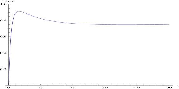
Figure 1. Soliton solution of the rotational elasticity.

In the static case, the equations of motion reduce to the single ODE

(3.13) $${\lambda}_{1}(r^{2}w^{\prime})^{\prime}+U(w)=0.$$

For ${\lambda}_{2}=2{\lambda}_{1}$ this further reduces to $(r^{2}w^{\prime})^{\prime}+\sin(2w)=0$, whereas when ${\lambda}_{2}={\lambda}_{1}$ one is left with $(r^{2}w^{\prime})^{\prime}-{\frac{1}{2}}\sin(4w)=0$. The qualitative analysis of the equation (3.13) reveals the existence of static solutions that vanish at $r=0$ and approach asymptotically $\pi/4$ at infinity for $r\rightarrow\infty$.

Numerical integration is straightforward. The form of the solution depends on the coupling constants and on the initial value of $w^{\prime}(0)$. However, the qualitative behaviour remains the same. As a specific example, Fig. 1 presents the soliton for ${\lambda}_{2}={\lambda}_{1}$ when $w^{\prime}(0)=1$.

In the static case we can introduce the new function $f$, defined by

(3.14) $$w=\frac{1}{2}\arctan\{\sinh(f(\log(r)))\}$$

which transforms (3.10) into an autonomous second order differential equation

(3.15) $$f_{\beta\beta}+f_{\beta}(1-\tanh(f)f_{\beta})-2\sinh(f)-4\tanh(f)+2\frac{\lambda_{2}}{\lambda_{1}}(\sinh(f)+\tanh(f))=0,$$

where $\beta=\log(r)$. This equation can now be analysed using standard techniques from ordinary differential equations or dynamical systems, and we find that this static system has three equilibrium points

(3.16) $$f=0,\qquad\sinh f=\pm\frac{\sqrt{\lambda_{1}}\sqrt{3\lambda_{1}-2\lambda_{2}}}{\lambda_{1}-\lambda_{2}},$$

with eigenvalues $(0,-1)$ in all three cases which in turn yields interesting (in)stability properties.

4. Discussion

The rotational elasticity model has many features similar to the model suggested by Skyrme [59]. Although the Lagrangians are different, the dynamics looks qualitatively the same. In particular, the remarkable feature of the rotational elasticity is the existence of solitons which are close relatives to the Skyrmions. The topological nature of such configurations (which we demonstrate below) guarantees the stability of solutions obtained in the sense that the variations of the coframe and connection cannot change the value of the conserved charge. Moreover, the moduli space of these solutions is obviously compact.

Recently it was noticed [54] that in the framework of the gauge approach in gravity and elasticity (that underlies the model under consideration, see Sec. 1.3) one can define an identically conserved current 3-form that gives rise to the topological charge that naturally classifies the field configurations. Such a 3-current “lives” on the 4-dimensional spacetime that is constructed as a foliation where the $t=const$ slices coincide with the manifold $\mathcal{M}$. Specialising to the case of the Weitzenböck geometry with the flat curvature (1.1), this topological current reduces to

(4.1) $$J^{\rm top}=K_{\alpha}{}^{\beta}\wedge\tilde{D}K_{\beta}{}^{\alpha}+{\frac{2}{3}}\,K_{\alpha}{}^{\beta}\wedge K_{\beta}{}^{\gamma}\wedge K_{\gamma}{}^{\alpha}.$$

Here $K_{\alpha}{}^{\beta}=\Gamma_{\alpha}{}^{\beta}-\tilde{\Gamma}_{\alpha}{}^{\beta}$ is the contortion defined as the difference between the Riemann-Cartan and the Riemannian connections. This 3-form is identically conserved on the 4-spacetime, $dJ^{\rm top}\equiv 0$ in view of (1.1). As a result, we can construct the topological charge

(4.2) $${\mathcal{Q}}={\frac{1}{96\pi^{2}}}\int K_{\alpha}{}^{\beta}\wedge K_{\beta}{}^{\gamma}\wedge K_{\gamma}{}^{\alpha}.$$

The integral is taken over the 3-manifold $\mathcal{M}$. The topological nature of the charge (4.2) and current (4.1) is manifested in the fact that the corresponding conservation law does not depend on any dynamics of the fundamental fields $\vartheta^{\alpha}$ and $\Gamma_{\alpha}{}^{\beta}$ [54].

The integral (4.2) is taken over the whole 3-space and the result is a constant for configurations that we studied in the previous section when $w$ vanishes at the origin and approaches constant value at infinity. Specializing to the connection gauge (1.14), we have $\tilde{\Gamma}_{\alpha}{}^{\beta}=0$ (the coframe is “gauged away”: $h^{\alpha}_{i}=\delta^{\alpha}_{i}$) and hence

(4.3) $${\mathcal{Q}} = {\frac{1}{96\pi^{2}}}\int\Gamma_{\alpha}{}^{\beta}\wedge\Gamma_{\beta}{}^{\gamma}\wedge\Gamma_{\gamma}{}^{\alpha}$$

$$= {\frac{1}{96\pi^{2}}}\int(\Lambda d\Lambda^{-1})_{\alpha}{}^{\beta}\wedge(\Lambda d\Lambda^{-1})_{\beta}{}^{\gamma}\wedge(\Lambda d\Lambda^{-1})_{\gamma}{}^{\alpha}.$$

Fixing the asymptotic boundary conditions so that $\Lambda^{\alpha}{}_{\beta}=\delta^{\alpha}_{i}u^{i}_{\beta}$ approaches unity near spatial infinity allows for the standard compactification [54] of the space $\mathcal{M}\approx\mathbb{S}^{3}$. We thus verify that the charge (4.2), (4.3) is a degree (“winding number”) of the maps $\Lambda:\mathbb{S}^{3}\rightarrow SO(3)$ which are classified by the integer numbers that are the elements of the third homotopy group $\mathbb{Z}=\pi_{3}(SO(3))$. By direct computation we can verify that $\mathcal{Q}=1$ for the soliton solution described above.

Construction of a multi-soliton generalisation is an interesting problem. One can approach this along the lines proposed in [54]. As a first step, we can replace the ansatz (3.1) by taking instead of (2.23) the orthogonal matrix that is a product of $N$ factors

(4.4) $$u_{\alpha}^{i}=\left(u_{(1)}\cdot u_{(2)}\cdot\dots\cdot u_{(N)}\right)_{\alpha}^{i}.$$

The dot denotes the usual matrix product. Such an ansatz would obviously generate a topological solution with the higher charge $\mathcal{Q}=N$. The construction of the multi-soliton configurations is a more nontrivial problem which one could try to solve by using the instanton technique.

The realization of the current theoretical model in the condensed matter systems is an interesting physical problem. The geometric constraint (1.1) of the vanishing curvature rules out the disclinations. It was shown in [54] that dislocations are also not relevant to the point-like soliton solutions. The solitons of this type are mentioned by Unzicker [64], who calls them a “Shankar monopole” [58] that describes a point-like defect in a $A$-phase superfluid Helium-3, [65, 46, 66]. As we mentioned already, our microrotational elasticity model belongs to the class of the so-called micropolar elasticity theories. The relevant physical continua describe, in particular, liquid crystals with rigid molecules, superfluids, rigid suspensions, blood fluid with rigid cells, magnetic fluids, dust fluids etc. Eringen [19] (see also references therein) extensively studied micromorphic, microstretch and micropolar elasticity models with other defects beyond the dislocations and disclinations. We refer again to the paper of Randono and Hughes [54] where the point-like topological solution (called there a torsional monopole) is depicted and a possible physical manifestations of such structures are qualitatively related to certain nontrivial electronic behaviour of condensed matter systems with strong spin-orbit coupling such as (1+3)-dimensional topological insulators. A careful quantitative analysis of such possibilities will be left for a future study.

Acknowledgments

We thank Dmitri Vassiliev and Friedrich Hehl for discussions and advice. We also thank the referees for their valuable reports.

References

- [1] Yu.A. Amenzade, Theory of elasticity (Mir Publishers, Moscow, 1979).
- [2] B.A. Bilby, R. Bullough, and E. Smith, Continuous distributions of dislocations: a new application of the methods of non-Riemannian geometry, Proc. Roy. Soc. London A 231 (1955) 263-273.
- [3] C.G. Böhmer, R. Downes, and D. Vassiliev, Rotational elasticity, The Quarterly Journal of Mechanics and Applied Mathematics 64 (2011) 415-439; arXiv:1008.3833.
- [4] C.G. Böhmer, Modelling rotational elasticity with orthogonal matrices, (2010) 10 pp.; arXiv:1008.4005.
- [5] O.M. Braun and Y.S. Kivshar, Nonlinear dynamics of the Frenkel-Kontorova model, Phys. Rept. 306 (1998) 1-108.
- [6] G. Capriz, Continua with microstructure, Springer Tracts in Natural Philosophy 35 (springer, Berlin, 1989).
- [7] O. Chervova and D. Vassiliev, The stationary Weyl equation and Cosserat elasticity, J. Phys. A: Math. Theor. 43 (2010) 335203 (14 pages); arXiv:1001.4726.
- [8] E. Cosserat and F. Cosserat, Théorie des corps déformables (Paris: Hermann, 1909); English translation by D.H. Delphenich available at http://www.uni-due.de/hm0014/Cosserat_files/Cosserat09_eng.pdf.
- [9] P.G. De Gennes and J. Prost, The physics of liquid crystals, 2nd ed. (Clanderon Press, Oxford, 1993).
- [10] G.H. Derrick, Comments on nonlinear wave equations as models for elementary particles, J. Math. Phys. 5 (1964) 1252-1254.
- [11] J. Dyszlewicz, Micropolar theory of elasticity, Lecture Notes in Applied and Computational Mechanics, v. 15 (Springer, Berlin, 2004).
- [12] D.G.B. Edelen and D.C. Lagoudas, Gauge theory and defects in solids, “Mechanics and Physics of Discrete System”, Vol. 1, G.C. Sih, ed. (North-Holland, Amsterdam, 1988).
- [13] J.L. Ericksen and C. Truesdell, Exact theory of stress and strain in rods and shells, Arch. Rat. Mech. Anal. 1 (1957) 295-323.
- [14] J.L. Ericksen, Hydrostatic theory of liquid crystals, Arch. Rational Mech. Anal. 9 (1962) 379-394.
- [15] J.L. Ericksen, Kinematics of macromolecules, Arch. Rational Mech. Anal. 9 (1962) 1-8.
- [16] J.L. Ericksen, Twisting of liquid crystals,J. Fluid Mech. 27 (1967) 59-64.
- [17] A.C. Eringen and E. S. Suhubi, Nonlinear theory of simple microelastic solids I, Int. J. Eng. Sci. 2 (1964) 189-204; Nonlinear theory of simple microelastic solids II, Int. J. Eng. Sci. 2 (1964) 389-404.
- [18] A.C. Eringen, editor, Continuum physics, Vol. IV, Polar and nonlocal field theories (Academic Press, New York, 1976).
- [19] A.C. Eringen, Microcontinuum field theories: I. Foundations and solids (Springer, New York, 1999).
- [20] J. Frenkel and T. Kontorowa, On the theory of plastic deformation and twinning, Physikalische Zeitschrift der Sowjetunion 13 (1938) 1-10.
- [21] A. E. Green, Multipolar continuum mechanics, Arch. Rational Mech. Anal. 17 (1964) 113-147.
- [22] G. Grioli, Elasticità asimmetrica, Ann. Mat. pura e Appl. 50 (1960) 389-417.
- [23] G. Grioli, Contributo per una formulazione di tipo integrale della meccanica dei continui di Cosserat, Ann. Mat. pura e Appl. 111 (1976) 175-183.
- [24] G. Grioli, Microstructures as a refinement of Cauchy theory. Problems of physical concreteness, Continuum Mechanics and Thermodynamics 15 (2003) 441-450.
- [25] F. Gronwald and F.W. Hehl, Stress and hyperstress as fundamental concepts in continuum mechanics and in relativistic field theory, In: G. Ferrarese, ed., “Advances in Modern Continuum Dynamics”, International Conference in Memory of Antonio Signorini, Isola d’Elba, June 1991, pp. 1-32. Pitagora Editrice, Bologna (1993); arXiv:gr-qc/9701054.
- [26] F.W. Hehl and Yu.N. Obukhov, Foundations of classical electrodynamics: Charge, flux, and metric (Birkhäuser: Boston, 2003).
- [27] F.W. Hehl and Yu.N. Obukhov, Élie Cartan’s torsion in geometry and in field theory, an essay, Ann. Fond. Louis Broglie 32 (2007) 157-194; arXiv:0711.1535.
- [28] F.W. Hehl, J.D. McCrea, E.W. Mielke, and Y. Ne’eman, Metric-affine gauge theory of gravity: Field equations, Noether identities, world spinors, and breaking of dilation invariance, Phys. Repts 258 (1995) 1-171.
- [29] A. Kadic and D.G.B. Edelen, A gauge theory of dislocations and disclinations, Lecture Notes in Physics, Vol. 174 (Springer, Berlin, 1983).
- [30] E. Kröner, editor, Mechanics of generalized continua, Proc. IUTAM Symp. Fredenstadt-Stuttgart, 1967 (Springer, Berlin, 1967).
- [31] E. Kröner, Continuum theory of defects, in: “Physics of defects”, Les Houches NATO Summer School, 35th session, 28 July - 29 August 1980; Eds. R. Balian, M. Kléman, J.-P. Poirier (North-Holland: Amsterdam, 1981), pp. 215-315.
- [32] M.O. Katanaev and I.V. Volovich, Theory of defects in solids and three-dimensional gravity, Ann. Phys. (USA) 216 (1992) 1-28.
- [33] M.O. Katanaev, Wedge dislocation in the geometric theory of defects, Theor. Math. Phys. 135 (2003) 733-744.
- [34] M.O. Katanaev, Geometric theory of defects, Phys. Uspekhi 48 (2005) 675-701 [Usp. Fiz. Nauk 175 (2005) 705-733, in Russian]; arXiv:cond-mat/0407469.
- [35] K. Kondo, On the geometrical and physical foundations of the theory of yielding, in: Proceedings of the 2nd Japan National Congress for Applied Mechanics, (Science Council of Japan: Tokyo, 1952) pp. 41-47.
- [36] K. Kondo, On the analytical and physical foundations of the theory of dislocations and yielding by the differential geometry of continua, Int. J. Engin. Sci. 2 (1964) 219-251.
- [37] T. Kontorova and J. Frenkel, On the theory of plastic deformation and twinning, Zh. Exp. Teor. Fiz. (ZHETF) 8 (1938) 89-95, 1340-1348, 1349-1358 (in Russian).
- [38] M. Lazar, The gauge theory of dislocations: a uniformly moving screw dislocation, Proc. Roy. Soc. Lond. A 465 (2009) 2505-2520.
- [39] M. Lazar and C. Anastassiadis, The gauge theory of dislocations: Static solutions of screw and edge dislocations, Phil. Mag. 89 (2009) 199-231.
- [40] M. Lazar and F.W. Hehl, Cartan’s spiral staircase in physics and, in particular, in the gauge theory of dislocations, Found. Phys. 40 (2010) 1298-1325; arXiv:0911.2121.
- [41] M. Lazar, On the fundamentals of the three-dimensional translation gauge theory of dislocations, Mathematics and Mechanics of Solids 16 (2011) 253-264; arXiv:1003.3549.
- [42] C. Malyshev, The T(3)-gauge model, the Einstein-like gauge equation, and Volterra dislocations with modified asymptotics, Ann. Phys. (USA) 286 (2000) 249-277.
- [43] C. Malyshev, The Einsteinian T(3)-gauge approach and the stress tensor of the screw dislocation in the second order: Avoiding the cut-off at the core, J. Phys.: Math. and Theor. A40 (2007) 10657-10684.
- [44] G.A. Maugin, On the structure of the theory of polar elasticity, Phil. Trans. R. Soc. Lond. A356 (1998) 1367-1395.
- [45] G.A. Maugin, Configurational forces: Thermodynamics, physics, mathematics, and numerics (CRC/Chapman & Hall: Boca Raton, 2011).
- [46] N.D. Mermin, The topological theory of defects in ordered media, Rev. Mod. Phys. 51 (1979) 591-648.
- [47] R.D. Mindlin, Micro-structure in linear elasticity, Arch. Rat. Mech. Anal. 16 (1964) 51-78.
- [48] D. Natroshvili, L. Giorgashvili and I.G. Stratis, Mathematical problems of the theory of elasticity of chiral materials, Applied Mathematics, Informatics and Mechanics 8 (2003) 47-103.
- [49] D. Natroshvili, L. Giorgashvili and I.G. Stratis, Representation formulae of general solutions in the theory of hemitropic elasticity, Q. Jl Mech. Appl. Math. 59 (2006) 451-474.
- [50] D. Natroshvili, R. Gachechiladze, A. Gachechiladze and I.G. Stratis, Transmission problems in the theory of elastic hemitropic materials, Applicable Analysis 86 (2007) 1463-1508.
- [51] P. Neff, Geometrically exact Cosserat theory for bulk behaviour and thin structures. Modelling and mathematical analysis, Habilitation Thesis (Darmstadt Tech. Univ., Darmstadt, 2004).
- [52] W. Nowacki, Theory of asymmetric elasticity, 2nd ed. (Pergamon, Oxford, 1985).
- [53] O.H. Olsen and M.R. Samuelsen, Rotationally symmetric breather-like solutions to the sine-Gordon equation, Phys. Lett. A77 (1980) 95-99.
- [54] A. Randono and T.L. Hughes, Torsional monopoles and torqued geometries in gravity and condensed matter, Phys. Rev. Lett. 106 (2011) 161102 (4 pages); arXiv:1010.1031.
- [55] H. Schaefer, Das Cosserat Kontinuum, ZAMM 47 (1967) 485-498.
- [56] H. Schaefer, Analysis der Motorfelder im Cosserat-Kontinuum, ZAMM 47 (1967) 319-328.
- [57] H. Schaefer, Die Motorfelder des dreidimensionalen Cosserat-Kontinuums im Kalkül der Differentialformen, Lecture course No. 19, International Centre for Mechanical Sciences (ICMS, Udine, 1970) 1-60.
- [58] R. Shankar, Applications of topology to the study of ordered systems, J. de Physique 38 (1977) 1405-1412.
- [59] T.H.R. Skyrme, A non-linear field theory, Proc. Roy. Soc. London A260 (1961) 127-138.
- [60] I.S. Sokolnikoff, Mathematical theory of elasticity (McGraw-Hill, New York, 1956).
- [61] R.A. Toupin, Elastic materials with couple-stresses, Arch. Rat. Mech. Anal. 11 (1962) 385-414.
- [62] R.A. Toupin, Theories of elasticity with couple-stress, Arch. Rat. Mech. Anal. 17 (1964) 85-112.
- [63] C. Truesdell and R. Toupin, The classical field theories. Encyclopedia of Physics, Vol. III/1. (Berlin-Göttingen-Heidelberg: Springer, 1960).
- [64] A. Unzicker, Topological defects in an elastic medium: A valid model particle physics, in: “Structured media”, Proc. Int. Symp. in memory of E. Kröner, Poznań, September 16-21, 2001; ed. B.T. Maruszewski (Publ. House Poznań Univ. of Technology, 2002) pp. 293-311.
- [65] D. Vollhardt and P. Wölfle, The superfluid phases of Helium 3 (Taylor & Francis: London, 1990).
- [66] G.E. Volovik, The universe in a Helium droplet (Clarendon Press: Oxford, 2003).
- [67] E. Whittaker, A history of the theories of aether and electricity (Thomas Nelson and Sons, London, United Kingdom, 1951), p 140.
- [68] A. Zeghadi, S. Forest, A.-F. Gourgues, and O. Bouaziz, Cosserat continuum modelling of grain size effects in metal polycrystals, Proc. Appl. Math. Mech. 5 (2005) 79-82.