Spectral properties of the three-dimensional Hubbard model

Abstract

We present momentum resolved single-particle spectra for the three-dimensional Hubbard model for the paramagnetic and antiferromagnetically ordered phase obtained within the dynamical cluster approximation. The effective cluster problem is solved by continuous-time Quantum Monte Carlo simulations. The absence of a time discretization error and the ability to perform Monte Carlo measurements directly in Matsubara frequencies enable us to analytically continue the self-energies by maximum entropy, which is essential to obtaining momentum resolved spectral functions for the Néel state. We investigate the dependence on temperature and interaction strength and the effect of magnetic frustration introduced by a next-nearest-neighbor hopping. One particular question we address here is the influence of the frustrating interaction on the metal-insulator transition of the three-dimensional Hubbard model.

I Introduction

One of the paradigms for correlation effects and competing orders in solid state physics is the Hubbard model Hubbard (1963); Gutzwiller (1963); Kanamori (1963)

$$H= -t\sum\limits_{\langle i,j\rangle\sigma}c^{\dagger}_{i\sigma}c^{\phantom{\dagger}}_{j\sigma}-t^{\prime}\sum\limits_{\langle\langle i,j\rangle\rangle\sigma}c^{\dagger}_{i\sigma}c^{\phantom{\dagger}}_{j\sigma}$$

$$+U\sum\limits_{i}\left(n_{i\uparrow}-\frac{1}{2}\right)\left(n_{i\downarrow}-\frac{1}{2}\right)\;.$$ (1)

The operators $c^{\dagger}_{i\sigma}$ ($c_{i\sigma}$) create (annihilate) an electron with spin $\sigma\in\{\uparrow,\downarrow\}$ at lattice site $i$, $n_{i\sigma}=c^{\dagger}_{i\sigma}c_{i\sigma}$ is the particle number operator, $t$ describes the hopping between neighboring sites (denoted by $\langle i,j\rangle$), $t^{\prime}$ the hopping between next-nearest neighbors (denoted by $\langle\langle i,j\rangle\rangle$) and $U$ implements the local Coulomb repulsion.

The Hubbard model, despite its simple structure, can only be solved exactly in one Essler et al. (2005) and infinite Georges et al. (1996) spatial dimensions. There are several expectations one can deduce from general energetic arguments and in particular from the connection between the Hubbard model and the Heisenberg hamiltonian in the limit of large interaction strength $t/U\to 0$.Fulde (1991) For a three-dimensional simple-cubic lattice and $t^{\prime}=0$, the Hubbard model at half filling shows antiferromagnetic order at finite temperature for any value $U>0$. The doubling of the unit cell causes this ordered state to be an insulator. With increased next-nearest-neighbor hopping this transition is suppressed and a Mott-Hubbard metal-insulator transition (MH-MIT) is expected to appear in the paramagnetic state at some non-zero critical value $U_{c}$ of the interaction.

Quantum Monte Carlo (QMC) methods are powerful tools that enable the controlled calculation of properties of large interacting quantum many-particle systems. Examples include spin models and many bosonic systems. However, simulations of fermionic models away from particle-hole symmetry are often severely hampered by the fermionic sign problem.Troyer and Wiese (2005) In particular, the identification of ordered phases, which requires a reliable finite-size scaling, becomes exceedingly complicated. Independent of the sign problem, the direct investigation of the properties of ordered phases possibly present in the thermodynamic limit is not possible, since any QMC simulation is performed on a finite system which cannot exhibit a spontaneously broken symmetry.

Therefore an approximation scheme allowing (i) calculations in the thermodynamic limit while (ii) including dynamical correlations in a controlled way is highly desirable. The dynamical mean-field theory (DMFT) Georges et al. (1996); Kotliar et al. (2006) and its cluster extensions Maier et al. (2005a) are such theories. The DMFT maps the lattice problem onto an effective single-site impurity model, at the cost of neglecting non-local many-body correlation effects. In many cases, the sign problem of the resulting impurity model is either absent or manageable. However, these non-local correlation effects are often crucial for the interplay between Fermi liquid and more exotic states of matter. Cluster mean-field theories are extensions of the DMFT to finite clusters, re-introducing non-local (short-ranged) correlations in a systematic manner but at the same time increasing the complexity of a simulation. In the limit of infinite cluster size they become exact. The controlled extrapolation of cluster results to the thermodynamic limit is often feasible in practice.Fuchs et al. (2011); Gull et al. (2011a)

DMFT has proven to be a very powerful tool for studying the fundamental aspects of the MH-MIT Kotliar et al. (2006). Within the DMFT, however, the MH-MIT is completely hidden inside an antiferromagnetic phase, which is insulating by symmetry.Pruschke and Zitzler (2003) Introducing magnetic frustration, e. g., by a non-zero $t^{\prime}$, tends to suppress the magnetic order and shift the critical interaction strength $U_{c}$ toward lower values. Thus the MH-MIT eventually emerges from the antiferromagnetic phase for large values of $t^{\prime}$.Peters and Pruschke (2009a)

In low-dimensional systems (single site) DMFT is in general not a good approximation. In particular, for the one-dimensional Hubbard model, non-local correlations are in fact dominant,Koch et al. (2008) leading to a complete breakdown of Fermi liquid physics and the formation of a novel low-energy fixed point, the Luttinger liquid.Essler et al. (2005) Similarly, in two dimensions a strong influence of spin fluctuations in the Hubbard model is expected, in particular at and close to half filling. Since the Mermin-Wagner theorem forbids the formation of an ordered state in two dimensions at finite temperature, the existing strong magnetic correlations will lead to correspondingly strong dynamical fluctuations at $T>0$ and will possibly trigger a similar breakdown of Fermi liquid physics as in the one-dimensional case. Evidence for this behavior has indeed been observed in various numerical simulations.Dagotto (1994); Maier et al. (2005a); Moukouri and Jarrell (2001); Onoda and Imada (2003); Parcollet et al. (2004); Hanasaki and Imada (2006); Zhang and Imada (2007); Liebsch et al. (2008); Gull et al. (2008a); Park et al. (2008); Gull et al. (2009); Werner et al. (2009)

The importance of short-ranged correlations in the three-dimensional Hubbard model is less clear and less well studied, and detailed studies of the phase diagram at high temperature have only recently begun to appear.De Leo et al. (2011); Fuchs et al. (2011) On the one hand, the precise value of the Néel temperature and critical exponents for the transition into the antiferromagnetic state will be directly influenced by the presence of spin fluctuations.Kent et al. (2005a) Since the antiferromagnetically ordered phase is an insulator, we expect the antiferromagnetic spin fluctuations in the paramagnetic phase to stabilize the MH-MIT, thus shifting the critical $U_{c}$ toward lower values. Adding frustration by, e. g., next-nearest-neighbor hopping $t^{\prime}$ will further enhance this effect. One may surmise that the MH-MIT will eventually emerge from the antiferromagnetic phase as in DMFT. To our knowledge this has not yet been investigated in detail.

In this work we study the Hubbard model for a three-dimensional cubic lattice using the dynamical cluster approximation (DCA) Hettler et al. (1998); Maier et al. (2005b) cluster dynamical mean-field algorithm on clusters of size $18$. We present momentum resolved single-particle spectra in the paramagnetic and in the antiferromagnetic phase, and investigate the influence of frustration effects caused by a next-nearest-neighbor hopping $t^{\prime}$. We focus our investigation on the interplay of frustration and spin fluctuations in the vicinity of the paramagnetic metal insulator transition.

II Method

We study the Hubbard model in three dimensions within the DCA to include both the short- to medium-ranged antiferromagnetic fluctuations and the possibility of actual long-range antiferromagnetic order. Since the DCA maps the lattice problem onto an effective periodic cluster coupled to a dynamic bath, numerically exact quantum Monte-Carlo (QMC) algorithms are ideally suited to solving this effective model.

Of particular interest in correlated electron systems are dynamical correlation functions such as single-particle spectra. However, QMC provides data only on the imaginary time or frequency axis, and the necessary analytic continuation of these data has proven to be difficult. The standard tool used to solve this problem is the maximum entropy method (MEM).Jarrell and Gubernatis (1996)

Previously, the quasi-standard for simulations of fermionic many-particle systems was the Hirsch-Fye algorithm,Hirsch and Fye (1986) which uses a discretization of the imaginary time axis. An alternative has evolved in recent years by the development of QMC algorithms in continuous imaginary time.Rubtsov and Lichtenstein (2004); Rubtsov et al. (2005); Gull et al. (2008b); Werner et al. (2006); Gull et al. (2010) The absence of a time discretization error and the possibility of Monte Carlo measurements directly in Matsubara frequencies Rubtsov and Lichtenstein (2004) enhance the quality of the data significantly Gull et al. (2007) and hence enable us to directly analytically continue self-energies.Wang et al. (2009) This avoids the extraction of the self-energies from already continued Green’s functions by a numerically difficult multi-dimensional root finding algorithm.Jarrell et al. (1995) In this paper we use an implementation of the continuous-time interaction expansion (CT-INT) QMC algorithm initially described by Rubtsov and co-workers Rubtsov and Lichtenstein (2004); Rubtsov et al. (2005) which performs a systematic expansion in the interaction term of the Hamiltonian.

For a simple cubic lattice in three dimensions the dispersion including nearest- and next-nearest- neighbor hopping reads

$$\epsilon_{\boldsymbol{k}}=-2t\sum\limits_{i=1}^{3}\cos(k_{i})-4t^{\prime}\left[\cos(k_{1})\cos(k_{2})\right.\\ \left.+\cos(k_{2})\cos(k_{3})+\cos(k_{1})\cos(k_{3})\right]\;,$$ (2)

where ${\boldsymbol{k}}=(k_{1},k_{2},k_{3})$ is an element of the first Brillouin zone of the simple cubic lattice. The full bandwidth

$$W=\begin{cases}12t&\mbox{for }|t^{\prime}|\leq t/4\;,\\ 8t+16|t^{\prime}|&\mbox{for }|t^{\prime}|>t/4\;,\\ \end{cases}$$ (3)

of this dispersion is used as the energy scale in this paper.

Let us briefly recall the essential aspects of the DCA. The central quantity is the single particle Green’s function in imaginary time $\tau$, defined by

$$G_{\sigma ij}(\tau)=-\langle\mathcal{T}c_{\sigma i}(\tau)c^{\dagger}_{\sigma j}\rangle\ .$$ (4)

Here $\mathcal{T}$ is the imaginary-time ordering operator, $\langle\cdot\rangle$ denotes a thermal expectation value, and $c_{\sigma i}(\tau)=e^{-H\tau}c_{\sigma i}e^{H\tau}$. The spatial and temporal Fourier transform of Green’s function is

$$G_{\sigma\boldsymbol{k}}({\rm i}\omega_{n}) =\frac{1}{N}\sum\limits_{ij}\exp\left[{\rm i}{\boldsymbol{k}}({\boldsymbol{R}}_{i}-{\boldsymbol{R}}_{j})\right]\times$$

$$\times\int\limits_{0}^{\beta}\!{\rm d}\tau\,\exp\left({\rm i}\omega_{n}\tau\right)G_{\sigma ij}(\tau)\;,$$ (5)

where $\boldsymbol{k}$ is located in the first Brillouin zone and $\omega_{n}=(2n+1)\pi/\beta$ with $n\in\mathbb{Z}$ and $\beta=1/k_{\mathrm{B}}T$ denotes the fermionic Matsubara frequencies. $T$ is the temperature, and $k_{\mathrm{B}}$ the Boltzmann’s constant. With Dyson’s equation, we write Green’s function as

$$G_{\sigma\boldsymbol{k}}(i\omega_{n})=\frac{1}{i\omega_{n}+\mu-\epsilon_{\boldsymbol{k}}-\Sigma_{\sigma\boldsymbol{k}}(i\omega_{n})}\;,$$ (6)

thus introducing the single-particle self-energy $\Sigma_{\sigma\boldsymbol{k}}(i\omega_{n})$ which contains all the many-body correlation effects in the system and, in general, is a function of both momentum $\boldsymbol{k}$ and energy $\omega_{n}$.

Within DCA, the full lattice model is approximated by a finite cluster of size $N$ embedded in a mean field. We tile the first Brillouin zone into $N$ non-overlapping cells, each represented by its central momentum $\boldsymbol{K}$ [see Fig. 1(b)

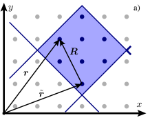
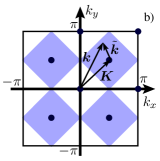
Figure 1: (Color online) Dynamical cluster approximation illustrated for an eight-site cluster in two dimensions. In real space (a) the origin of a cluster is labeled by $\tilde{\boldsymbol{r}}$. Each site of the cluster is identified by $\boldsymbol{R}$. A Fourier transformation maps the coordinate ${\boldsymbol{r}}=\tilde{\boldsymbol{r}}+{\boldsymbol{R}}$ of each lattice site to a vector $\boldsymbol{k}$ in the first Brillouin zone (b). The cluster momentum $\boldsymbol{K}$ now identifies the center of a cell in momentum space. All points inside this patch can be reached by $\tilde{\boldsymbol{k}}$. The DCA integrates out $\tilde{\boldsymbol{k}}$ and thus replaces the full $\boldsymbol{k}$ dependence of the lattice by the cells labeled by $\boldsymbol{K}$.

for an example]. The full $\boldsymbol{k}$-dependence of the model is approximated by the discrete set of $N$ cluster momenta $\boldsymbol{K}$ by setting $\Sigma_{\sigma\boldsymbol{k}}({\rm i}\omega_{n})\approx\Sigma_{\sigma\boldsymbol{K}}({\rm i}\omega_{n})$. Averaging over the volume $V$ of the cell corresponding to cluster momentum $\boldsymbol{K}$, one obtains the quantity

$$\bar{G}_{\sigma\boldsymbol{K}}({\rm i}\omega_{n})=\frac{1}{V}\int\!{\rm d}\tilde{{\boldsymbol{k}}}\frac{1}{{\rm i}\omega_{n}+\mu-\epsilon_{\boldsymbol{K}+\tilde{\boldsymbol{k}}}-\Sigma_{\sigma\boldsymbol{K}}({\rm i}\omega_{n})}\;,$$ (7)

which defines an effective non-interacting cluster via

$${\cal G}_{\sigma\boldsymbol{K}}({\rm i}\omega_{n})^{-1}=\bar{G}_{\sigma\boldsymbol{K}}({\rm i}\omega_{n})^{-1}+\Sigma_{\sigma\boldsymbol{K}}({\rm i}\omega_{n})\;.$$ (8)

With this set of quantities, a suitable method to solve the effective cluster defined by ${\cal G}_{\sigma\boldsymbol{K}}({\rm i}\omega_{n})$ and the interaction $U$, one can determine the self-energy $\Sigma_{\sigma\boldsymbol{K}}({\rm i}\omega_{n})$ iteratively as depicted in Fig. 2.

$${\cal G}_{\boldsymbol{K}}\ \longrightarrow\ \text{\framebox{QMC Cluster Solver}}\ \longrightarrow\ G_{\boldsymbol{K}}\vspace*{-3mm}$$

$$\uparrow$$

$$\downarrow$$

$$({\cal G}_{\boldsymbol{K}})^{-1}=(\bar{G}_{\boldsymbol{K}})^{-1}+\Sigma_{\boldsymbol{K}}\quad\quad\quad\Sigma_{\boldsymbol{K}}=({\cal G}_{\boldsymbol{K}})^{-1}-(G_{\boldsymbol{K}})^{-1}\vspace*{-1mm}$$

$$\uparrow$$

$$\downarrow$$

$$\bar{G}_{\boldsymbol{K}}=\frac{1}{V}\int\!{\rm d}\tilde{{\boldsymbol{k}}}\left(\mathrm{i}\omega_{n}+\mu-\epsilon_{{\boldsymbol{K}+\tilde{\boldsymbol{k}}}}-\Sigma_{\boldsymbol{K}}\right)^{-1}$$

Figure 2: Self-energy $\Sigma_{\sigma\boldsymbol{K}}({\rm i}\omega_{n})$ is determined self-consistently by iterating the depicted procedure until convergence is reached. The bottom line shows the calculation of the coarse-grained Green’s function $\bar{G}_{\boldsymbol{K}}$ by averaging over the momentum patch centered around $\boldsymbol{K}$ via integrating $\tilde{\boldsymbol{k}}$ over the volume $V$ of the patch. The dependency of Green’s functions and the self-energy on ${\rm i}\omega_{n}$ and $\sigma$ is omitted for simplicity.

From the QMC algorithm used to solve the effective cluster, we obtain the cluster Green’s function $\bar{G}_{\sigma\boldsymbol{K}}({\rm i}\omega_{n})$. Usually one then uses the maximum entropy method Jarrell and Gubernatis (1996) to analytically continue this quantity to the real axis. In order to be able to reverse the coarse-graining, i. e., calculate $G_{\sigma\boldsymbol{k}}(\omega+{\rm i}0^{+})$ for all $\boldsymbol{k}$ from the first Brillouin zone, one needs access to the self-energy $\Sigma_{\sigma\boldsymbol{K}}(\omega+{\rm i}0^{+})$ Maier et al. (2005a), which needs to be obtained by numerical inversion of Eq. 7. While this is feasible in the paramagnetic phase, the matrix structure appearing in the antiferromagnetically ordered phase (see section IV) renders this approach impractical.

We follow here an alternative route and analytically continue the self-energy instead Wang et al. (2009), which is related to the cluster Green’s function by

$$\Sigma_{\sigma\boldsymbol{K}}({\rm i}\omega_{n})={\cal G}_{\sigma\boldsymbol{K}}({\rm i}\omega_{n})^{-1}-G_{\sigma\boldsymbol{K}}({\rm i}\omega_{n})^{-1}\;,$$ (9)

i. e., an inversion of $G_{\sigma\boldsymbol{K}}({\rm i}\omega_{n})$. This inverse is calculated directly from the Monte Carlo bins using a jackknife procedure Miller (1974) and therefore incorporates a full error propagation of the covariance matrix. The bare Green’s function ${\cal G}_{\sigma\boldsymbol{K}}({\rm i}\omega_{n})$ is viewed here as an input parameter; and error propagation of errors contained in our estimate of it, which would require error propagation over subsequent iterations, is not considered here, such that all errors in ${\cal G}_{\sigma\boldsymbol{K}}({\rm i}\omega_{n})$ are neglected.

The analytic continuation of the self-energy from imaginary to real frequencies is then performed by the maximum entropy method, Jarrell and Gubernatis (1996) using a standard implementation of the algorithm following Bryan (1990). To accurately continue self-energies with MEM, their high frequency behavior has to be known Wang et al. (2009). To this end we perform a high-frequency expansion of the self-energy

$$\Sigma_{\sigma\boldsymbol{K}}({\rm i}\omega_{n})=\Sigma^{0}_{\sigma}+\frac{\Sigma^{1}_{\sigma}}{{\rm i}\omega_{n}}+\mathord{\mathcal{O}}(({\rm i}\omega_{n})^{-2})\;,$$ (10)

where the coefficients are given by (see AppendixA)

$$\Sigma^{0}_{\sigma}=U\left(\langle n_{-\sigma}\rangle-\frac{1}{2}\right)$$ (11)

and

$$\Sigma^{1}_{\sigma}=U^{2}\langle n_{-\sigma}\rangle\left(1-\langle n_{-\sigma}\rangle\right)\;.$$ (12)

We now define the quantity

$$\Sigma^{\prime}_{\sigma\boldsymbol{K}}({\rm i}\omega_{n}):=\frac{\Sigma_{\sigma\boldsymbol{K}}({\rm i}\omega_{n})-\Sigma_{\sigma}^{0}}{\Sigma_{\sigma}^{1}}\;.$$ (13)

Since the average number density $\langle n_{-\sigma}\rangle$ is a Monte Carlo measurement, we estimate $\Sigma^{\prime}_{\sigma\boldsymbol{K}}({\rm i}\omega_{n})$ and its covariance matrix by a jackknife procedure. The rescaled self-energy $\Sigma^{\prime}_{\sigma\boldsymbol{K}}({\rm i}\omega_{n})$ as function of Matsubara frequencies is related to the imaginary part $\text{Im}\,\Sigma^{\prime}_{\sigma\boldsymbol{K}}(\omega+i0^{+})$ on the real frequency axis through the Hilbert transform

$$\Sigma^{\prime}_{\sigma\boldsymbol{K}}({\rm i}\omega_{n})=-\frac{1}{\pi}\int\limits_{-\infty}^{\infty}\!{\rm d}\omega^{\prime}\frac{\text{Im}\,\Sigma^{\prime}_{\sigma\boldsymbol{K}}(\omega^{\prime})}{{\rm i}\omega_{n}-\omega^{\prime}}\;.$$ (14)

By virtue of the rescaling Eq. 13 we furthermore have

$$-\frac{1}{\pi}\int\limits_{-\infty}^{\infty}\!{\rm d}\omega\,\text{Im}\,\Sigma^{\prime}_{\sigma\boldsymbol{K}}(\omega)=1\;,$$ (15)

i. e., the spectral function $-\frac{1}{\pi}\text{Im}\,\Sigma^{\prime}_{\sigma\boldsymbol{K}}(\omega)$ is non-negative, normalized to unity, and can thus be calculated by the MEM from the data on the imaginary axis. The real part of the self-energy then follows from the Kramers-Kronig relation

$$\mbox{Re}\,\Sigma_{\sigma\boldsymbol{K}}(\omega)=-\frac{1}{\pi}\,\mbox{P}\!\!\!\int\limits_{-\infty}^{\infty}\!{\rm d}\omega^{\prime}\frac{\text{Im}\,\Sigma_{\sigma\boldsymbol{K}}(\omega^{\prime})}{\omega-\omega^{\prime}}+\Sigma^{0}_{\sigma}\;,$$ (16)

where $\mbox{P}\!\int$ denotes a principal value integral. An example for a full self-energy on the real-frequency axis is shown in Fig. 3(a).

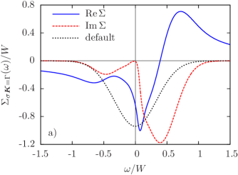
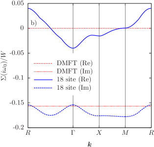
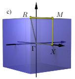
Figure 3: (Color online) (a) Self-energy on the real-frequency axis in the paramagnetic phase for $\boldsymbol{K}=\Gamma$, $U=W$, $t^{\prime}=0$, and $T=0.02\,W$ (a). The default model that entered the MEM calculation of the imaginary part is also shown. The real part is obtained from the imaginary part via Eq. 16. (b) Real and imaginary parts of the interpolated self-energy $\Sigma_{\boldsymbol{k}}(\mathrm{i}\omega_{0})$ for the smallest Matsubara frequency for an 18-site cluster, $U=0.67\,W$ and $T=0.03\,W$ at half filling. The self-energy values at momenta between the discrete cluster momenta are obtained from an interpolation using Akima splines Akima (1970) in three dimensions. The horizontal straight lines denote DMFT results. The interpolation follows the path along the high symmetry points of the first Brillouin zone depicted in panel (c). For an estimate of finite-size effects in (b) see also Ref. Gull et al. (2011a)

An interpolation of the coarse-grained self-energies yields the self-energy $\Sigma_{\sigma\boldsymbol{k}}(\omega)$ for all momenta $\boldsymbol{k}$ of the Brillouin zone. We use a three-dimensional interpolation based on Akima splines Akima (1970) which provide a smooth interpolation along the momentum points while avoiding spurious oscillations. Finally, the single-particle spectral function $A_{\sigma\boldsymbol{k}}(\omega)$ is calculated using Dyson’s equation:

$$A_{\sigma\boldsymbol{k}}(\omega)=-\frac{1}{\pi}\text{Im}\,\frac{1}{\omega+\mu-\epsilon_{\boldsymbol{k}}-\Sigma_{\sigma\boldsymbol{k}}(\omega)}\;.$$ (17)

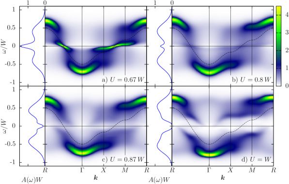
Figure 4: (Color online) Momentum resolved single-particle spectra for $T=0.02\,W$ and $t^{\prime}=0$. The momenta $\boldsymbol{k}$ follow a path along high symmetry directions of the first Brillouin zone as depicted in Fig. 3c. The left part of each diagram shows the local single-particle spectrum $A(\omega)$ derived from the direct analytic continuation of the Green’s function. The dashed line denotes the bare dispersion $\epsilon_{\boldsymbol{k}}$.

The quantity $A_{\sigma{\boldsymbol{k}}}(\omega)$could in principle also be calculated by an analytic continuation of the Green’s function at each cluster momentum $\boldsymbol{K}$ followed by an interpolation of the Green’s function values directly. However, this procedure approximates the exactly known momentum dependence of the dispersion $\epsilon_{\boldsymbol{k}}$, which causes a significant loss of momentum resolution. We will not consider it any further.

As an example, Fig. 3(b) shows the interpolated momentum-resolved self-energy for the smallest Matsubara frequency $\mathrm{i}\omega_{0}$ (full and dashed lines). The results were obtained for a cluster with 18 $\boldsymbol{K}$ momenta and a Coulomb repulsion $U=0.67\,W$ at $T=0.03\,W$. The comparison with the corresponding DMFT result (dotted lines) shows that the momentum resolution of the DCA adds significant $\boldsymbol{k}$ dependence to the self-energy. Thus the many-particle renormalizations acquire a significant $\boldsymbol{k}$ dependence in DCA, even for the three-dimensional Hubbard model at comparatively weak coupling.Fuchs et al. (2011); Gull et al. (2011a)

The available computational resources and the quality of data needed for high-precision analytic continuation, limit us to study clusters of comparatively small size. We limit ourselves to a study of a cluster of size $N=18$ described by the basis vectors ${\boldsymbol{a}}_{1}=(1,1,2)$, ${\boldsymbol{a}}_{2}=(2,2,-2)$, and ${\boldsymbol{a}}_{3}=(2,-1,-1)$. This cluster is the optimal bipartite cluster of this size Kent et al. (2005a) following the criteria proposed by Betts et al. Betts and Stewart (1997). Since we are primarily interested in identifying trends and basic physical effects, we do not perform calculations for larger clusters to obtain a finite-size scaling as would have been necessary, e.g., for a precise estimation of the equation of state or the Néel temperature in the thermodynamic limit.Kent et al. (2005a); Fuchs et al. (2011)

III Properties of the paramagnetic phase

We begin the discussion of our results by presenting spectral functions in the paramagnetic phase of the model, i.e., we manually suppress long-range order. This allows us to distinguish dynamical effects coming from fluctuations from effects caused by the (static) symmetry breaking.

III.1 Metallic phase

Figure 4 presents single-particle dispersions in the paramagnetic phase for $T=0.02\,W$, $t^{\prime}=0$ and four different Coulomb repulsions $U=0.67W,U=0.8W,U=0.87W,$ and $U=W$. The selected $\boldsymbol{k}$ points follow a path along the high symmetry points of the first Brillouin zone depicted in Fig. 3(c). Local single particle spectra are shown on the left of each panel. For small $U=0.67\,W$ we observe a clear quasi-particle peak at the Fermi level, both in the density of states (DOS) and the spectral function. The momentum resolved spectra show that the main contributions to the quasi-particle peak are situated halfway between the $\Gamma$ and $R$ points and the $X$ and $M$ points, respectively. Comparison of the peak dispersion in these regions to the non-interacting dispersion (dashed line) reveals a clear flattening at the Fermi energy, i. e., an increased effective mass of the quasi-particles. At higher energies additional structures—the lower and upper Hubbard bands—are visible. They follow the curvature of the bare dispersion but are shifted to higher energies and connected to the quasi-particle band through broad “waterfall”-like pieces reminiscent of structures observed in angle-resolved photoemission spectroscopy of cuprates.Graf et al. (2007) For increasing Coulomb repulsion $U$ the quasi-particle band at the Fermi energy vanishes and is replaced by an insulating gap. At the same time the dispersion of the high-energy structures flattens: the system becomes more localized. Thus for the temperature studied a crossover from a metallic dispersion at $U=0.67\,W$ to a Mott insulating phase at $U=W$ is clearly visible. We will return to the details of the Mott-Hubbard metal-insulator transition in section III.2.

To make the influence of the momentum dependence of the self-energy in the spectra more transparent,

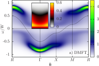
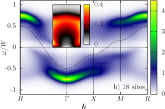
Figure 5: (Color online) Momentum resolved single-particle spectra for $T=0.02\,W$, $t^{\prime}=0$, and $U=0.93\,W$ using a non-dispersive DMFT self-energy (a) and a momentum dependent cluster self-energy (b). The inset highlights a part of the spectrum using an alternative color scheme.

Fig. 5 compares an insulating spectrum based on self-energies of the 18 site cluster to the corresponding spectrum based on a momentum-independent DMFT self-energy. While many overall features are similar, there are qualitative differences. For example, a blowup of the details of the spectra close to the $\Gamma$ point (insets to Fig. 5) shows that a substantial part of the DMFT spectrum around the $\Gamma$ point is located just above the Fermi energy. This contribution is shifted to higher frequencies in the cluster calculation, and the curvature is reversed, more resembling the structure of the lower Hubbard band but with much less spectral weight. The feature can be interpreted as a precursor of the complete symmetry with respect to the Fermi energy occurring for spectra in the antiferromagnetically ordered phase (see section IV). Thus, we attribute these pale reflections of the lower Hubbard band to the so-called shadow bands Kampf and Schrieffer (1990) arising due to antiferromagnetic fluctuations not contained in the DMFT simulation.

Next we examine the influence of a next-nearest neighbor hopping $t^{\prime}$. In quantum Monte Carlo calculations, a non-zero value of $t^{\prime}$ introduces a fermionic sign problem even at half filling that may lead to a significantly larger computational cost. However, for the temperatures, Coulomb repulsions and cluster size studied here the average sign is always greater than 0.94 and thus affects the efficiency of the simulations only marginally.

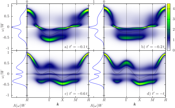
Figure 6: (Color online) Single-particle spectra for $U=0.67\,W$, $T=0.02\,W$ and non-zero $t^{\prime}$.

Fig. 6 shows results of calculations for $U=0.67\,W$ and different values for $t^{\prime}$. The particle-hole symmetric spectrum of Fig. 4(a) becomes more and more asymmetric with increasing $t^{\prime}$. We attribute most of these changes to the changes in the bare dispersion $\epsilon_{\boldsymbol{k}}$. However, while for small to moderate $t^{\prime}$ the quasi-particle properties do not seem to change much, one observes a significant reduction in the spectral weight at the Fermi energy for larger $t^{\prime}$, resulting in a reduction of the quasiparticle peak in the analytically continued spectra. For example, at $t^{\prime}=-t$ the integrated weight of the quasi-particle peak is reduced by 50% compared to the value for $t^{\prime}=0$ in Fig. 4(a). These observations indicate a reduction of the quasi-particle mass with increasing $t^{\prime}$, in accordance with previous DMFT findings Peters and Pruschke (2009a).

Frustration effects on the insulating spectrum in Fig. 4(d) ($U=W$) are illustrated in Fig. 7.

Figure 7: (Color online) Single-particle spectra for $U=W$, $T=0.02\,W$ and non-zero $t^{\prime}$.

As for the metallic spectrum, the features present in Fig. 4(d) for $t^{\prime}=0$ initially change only weakly and in particular the “shadow” structures seem to be present, albeit with reduced weight. For strong frustration, Hubbard bands become dominant. These Hubbard bands have a rather well-defined structure and dispersion reminiscent of the bare dispersion. Furthermore, a peak develops just below the Fermi energy, which becomes more pronounced with increasing $t^{\prime}$ and appears to have only small momentum dependence.

III.2 Mott-Hubbard Metal-Insulator Transition

One of the interesting properties of the Hubbard model is the formation of a correlation driven metal-insulator transition in the paramagnetic phase, the so-called Mott-Hubbard metal-insulator transition (MH-MIT). Different from the conventional band or Slater insulators for even electron number, where the insulating behavior is due to a completely filled band, the MH-MIT occurs in a partially filled band, which within a simple single-particle picture would thus be conducting. Such a transition is believed to frequently be present in transition metal oxides,Imada et al. (1998) and has been discussed both from an experimental and theoretical point of view over the past 50 years. Note that it is also different from the insulating state originating from an antiferromagnetic order; the latter implies a broken translational invariance and can hence be purely explained by band structure effects (see also section IV).

On a simple cubic lattice with only nearest-neighbor hopping the MH-MIT of the Hubbard model at half filling is completely covered by the antiferromagnetic phase.R. Staudt et al. (2000) Nevertheless, one may study it within a generalized mean-field theory by suppressing long-range antiferromagnetic order in the system. This is accomplished by enforcing translational symmetry on the bath and thereby preventing any symmetry-breaking. One of the clearest signs, numerically, for identifying the MH-MIT is given by the value of the DOS at the Fermi energy: A non-zero value at $T=0$ is indicative of a metal, a zero value of an insulator. Identifying the MIT at $T>0$ without a detailed analysis of the temperature dependence is more subtle, but again the DOS at the Fermi level can serve as “order parameter”: Away from the MH-MIT the DOS varies smoothly as function of temperature. When approaching the MH-MIT at half filling as function of $U$ or $T$, DMFT analyses suggest that the DOS will show a jump Georges et al. (1996); Moeller et al. (1995) below a critical end point. Furthermore, the transition is of first order with a nice hysteresis in the critical region. This behavior has been confirmed for two-dimensional systems within cluster DMFT on small Park et al. (2008) and larger Gull et al. (2009) clusters. Note that we do not discuss the approach to the MH-MIT as function of doping. The behavior of the system at this transition is very different, and has been addressed by a number of groups both in DMFT and cluster variants on a wide range of systems.Kotliar et al. (2002); Georges et al. (2004); Werner et al. (2009); Ferrero et al. (2009a, b); Gull et al. (2010); Lin et al. (2010); Sordi et al. (2010)

We estimate the density of states at the Fermi level from the low-frequency behavior of our Matsubara Green’s function $G_{ii}({\rm i}\omega_{n})$ that is available as direct Monte Carlo measurement and does not require analytic continuation. This approach is based on the relation

$$\beta G_{K}\left(\frac{\beta}{2}\right)=-\frac{\beta}{2}\int\limits_{-\infty}^{\infty}\!{\rm d}\omega\frac{A_{\boldsymbol{K}}(\omega)}{\cosh\frac{\beta}{2}\omega}\stackrel{{\scriptstyle\beta\to\infty}}{{\longrightarrow}}-\pi\,A_{\boldsymbol{K}}(0)$$ (18)

for the long-time behavior of the imaginary time Green’s function and the fact that the long-time behavior translates into the low-energy behavior under the Fourier transform.

Figure 8(a)

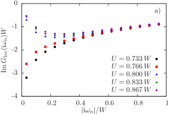
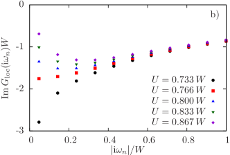
Figure 8: (Color online) Imaginary part of the local Green’s function in Matsubara frequencies for $t^{\prime}=0$, $T=0.01\,W$ (a) and $T=0.015\,W$ (b). Several values of $U$ around the MH-MIT are shown.

shows the imaginary part of $G_{\rm loc}({\rm i}\omega_{n}):=G_{ii}({\rm i}\omega_{n})$ for $t^{\prime}=0$ and $T=0.01\,W$ obtained within the DCA for a cluster size of 18. The jump from an insulating Green’s function at $U=0.80\,W$ to a metallic solution at $U=0.766\,W$ clearly shows the location of the MH-MIT at this temperature. For $T=0.015\,W$ we could only detect a crossover from insulating to metallic behavior [see Fig. 8(b)]. This indicates that the critical endpoint of the MH-MIT transition line is located between $T=0.01\,W$ and $T=0.015\,W$, substantially below the Néel temperature at this interaction strength [$T_{\rm N}=0.030(3)\,W$ at $U=0.8\,W$ R. Staudt et al. (2000); Kent et al. (2005a)].

Another observable that shows a clear signal of the MH-MIT is the effective mass, defined as

$$\frac{m^{\ast}_{\boldsymbol{k}}}{m}=1-\left.\frac{\partial Re\Sigma_{\sigma\boldsymbol{k}}(\omega)}{\partial\omega}\right|_{\omega=0}\;,$$ (19)

where $m$ denotes the bare carrier mass. The effective mass at non-zero (but sufficiently low) temperature may be estimated from the QMC without resorting to analytical continuations as Serene and Hess (1991)

$$\frac{m^{*}_{\boldsymbol{k}}}{m}\approx 1-\frac{\text{Im}\Sigma_{\sigma\boldsymbol{k}}({\rm i}\omega_{0})}{\omega_{0}}\;,$$ (20)

where $\omega_{0}$ is the lowest Matsubara frequency (see, e. g., Fig. $10$ in Ref. Gull et al. (2010) for a comparison between directly obtained and analytically continued estimates). At the MH-MIT, $m^{*}_{\boldsymbol{k}}$ across the Fermi surface exhibits a sharp increase.

The estimate for the effective mass obtained that way is shown in Fig. 9(a)

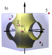
Figure 9: (Color online) (a) Quasi-particle mass $m^{*}_{\boldsymbol{K}}$ as function of mean distance $d$ from the Fermi surface in units of the lattice spacing $a$ (a). The distance $d_{\boldsymbol{K}}$ is defined as the average of the distances between the Fermi surface and all momenta in the cluster cell described by the cluster momentum $\boldsymbol{K}$. The 18 cluster momenta reduce to five different masses due to point symmetries. The labels 1 to 5 refer to the points depicted in panel (b), which also shows the non-interacting Fermi surface for $t^{\prime}=0$.

for two different values $U=0.73\,W<U_{c}(t^{\prime}=0)$ and $U=0.8\,W>U_{c}(t^{\prime}=0)$ and $t^{\prime}=0$ and $-0.2\,t$ at $T=0.01\,W$. We do not show the result for $m^{\ast}_{\boldsymbol{k}}$ from the interpolated data, as the division by $\omega_{0}$ with $\omega_{0}/W\ll 1$ also strongly enhances spurious artificial oscillations due to interpolation, but rather we present the masses $m^{*}_{\boldsymbol{K}}$ for each of the 18 cluster momenta as functions of their mean distance to the non-interacting Fermi surface for $t^{\prime}=0$. The mean distance is calculated by averaging the distance to the Fermi surface of all points inside the cluster cell around $\boldsymbol{K}$. Due to symmetry, some cluster momenta are equivalent and thus we obtain only five different effective masses. Figure 9(b) depicts one representative cluster momentum for each one of these five equivalence classes.

For both values of $t^{\prime}$ the ${\boldsymbol{K}}$ dependence of $m^{\ast}_{\boldsymbol{K}}$ for $U$ deep inside the metallic phase is rather weak, although nevertheless visible. The insulating phase, in contrast, shows a dramatic increase of the effective mass for the cluster momenta near the Fermi surface. For example, point 1 with the strongest enhancement is situated on the Fermi surface of the non-interacting system. Thus, the natural interpretation is that MH-MIT appears first for $\boldsymbol{k}$ points at or close to the Fermi surface. Points far away from the Fermi surface, on the other hand, like points 4 and 5 (5, for example, corresponding to $\Gamma$, respectively $R$), experience only weak renormalizations. The interpretation is further supported by the influence of non-zero $t^{\prime}$, which moderately modifies the mass due to changing distances of the cluster $\boldsymbol{K}$ points from the Fermi surface and a different critical $U_{c}$, but otherwise shows a similar behavior. We, however, do not observe a significant variation of $m^{\ast}_{\boldsymbol{K}}$ across the Fermi surface. The difference between points 1 and 2 in Fig. 9 can be explained by the large distance of the cluster center from the Fermi surface.

Note that this behavior of the three-dimensional model is different from the two-dimensional Hubbard model, where the Mott transition within DCA has been investigated in some detail.Werner et al. (2009); Gull et al. (2009, 2010) In this case, the so-called “momentum selective Mott transition” has been observed, where different parts of the Fermi surface undergo a metal insulator transition for different interaction strengths. To conclusively exclude the possibility of a momentum selective MH-MIT in three dimensions, larger clusters with a finer grid of $\boldsymbol{K}$ points on different parts of the Fermi surface would be needed.

In the following we focus on cluster momentum 1 in Fig. 9(b), which is situated directly on the Fermi surface, midway between $\Gamma$ and $M$. Since this point exhibits the strongest mass enhancement in the insulating phase, it is an ideal candidate for studying the MH-MIT. The effective mass of this $\boldsymbol{K}$ point is plotted in Fig. 10

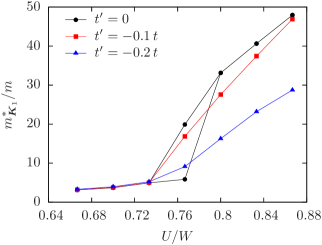
Figure 10: (Color online) Quasi-particle mass estimate $m^{*}_{\boldsymbol{K}_{1}}$ at the midpoint between $\Gamma$ and $M$ [point 1 in Fig. 9(b)], for $T=0.01\,W$ as function of the interaction parameter $U$.

as a function of $U$.

At $U_{\rm c}=0.766\,W$, both an insulating and a metallic solution can be stabilized, depending on the initial Green’s function used to start the DCA self-consistency. This behavior indicates a coexistence region in this regime of interaction parameters and tells us that the qualitative physical properties of the paramagnetic MH-MIT do not change at least qualitatively for a true three-dimensional system. The figure also shows the corresponding curves for next-nearest-neighbor hopping parameters $t^{\prime}=-0.1\,t$ and $t^{\prime}=-0.2\,t$. Here the coexistence region has vanished at the temperature for which the simulations were done, while the relatively smooth shape of the curve indicates that one is still observing a crossover and not yet a sharp phase transition as in the case of $t^{\prime}=0$. This is again in accordance with previous DMFT calculations, where a reduction of both the critical temperature and the critical value of $U$ was observed with increasing $t^{\prime}$.Peters and Pruschke (2009b) It is, however, different from the interaction transition in the two-dimensional Hubbard model,Gull et al. (2009) where increasing $|t^{\prime}|$ leads to an increase of the critical interaction strength.

It would be highly desirable to perform simulations at lower temperatures for non-zero $t^{\prime}$, but since the computational effort necessary increases dramatically with decreasing temperature, we were not yet able to do these simulations for the time being.

Previous studies of the interaction driven MH-MIT at non-zero temperature were largely performed on a Bethe lattice in the limit of infinite dimension within the DMFT approximation,Bulla et al. (2001); Joo and Oudovenko (2001) respectively, for a two-dimensional Hubbard model using the correlator projection method Onoda and Imada (2003); Hanasaki and Imada (2006) or cluster DMFT.Moukouri and Jarrell (2001); Parcollet et al. (2004); Zhang and Imada (2007); Liebsch et al. (2008); Gull et al. (2008a); Park et al. (2008); Gull et al. (2009); Werner et al. (2009) While the general features of the MH-MIT appear to be rather insensitive to the actual non-interacting band structure, the details like critical values for temperature and Coulomb interactions vary strongly with details of the model as well as the approximations involved in the computation and finite size effects.

To compare values for lattices with different noninteracting density of states $\rho(\omega)$, Bulla Bulla (1999) suggested using the second moment of the DOS

$$W_{\mathrm{eff}}=4\sqrt{\int\limits_{-W/2}^{W/2}\!{\rm d}\omega\,\omega^{2}\rho(\omega),}$$ (21)

as the characteristic energy scale instead of the bandwidth $W$. From Eq. (21) one obtains $W_{\mathrm{eff}}=W$ for the Bethe lattice and $W_{\mathrm{eff}}\approx 0.816\,W$ for the simple cubic lattice, and a rather good agreement of critical values when relating them to $W_{\mathrm{eff}}$.Bulla (1999); Žitko et al. (2009) Our result $U_{\mathrm{c}}=0.77(3)\,W$ for the coexistence region then translates to $U_{\mathrm{c}}=0.94(3)\,W_{\mathrm{eff}}$ at $T=0.012\,W_{\mathrm{eff}}$. For a conventional DMFT calculation, Refs. Bulla et al. (2001) and Joo and Oudovenko (2001) located the coexistence region for this temperature around $U_{c}=1.18(2)\,W_{\mathrm{eff}}$. This indicates that for a true three-dimensional system the critical values of the MH-MIT will be renormalized, and in particular the critical $U_{\mathrm{c}}$ will be shifted to lower values. We attribute these renormalizations to the short-ranged antiferromagnetic fluctuations present in the DCA. They will have the tendency to suppress the formation of quasi-particles and will thus cause the transition to shift to smaller Coulomb repulsions $U$. A detailed investigation of the location of the transition in the thermodynamic limit would require the study of a range of cluster sizes and a careful finite-size analysis along the lines of Refs. Kent et al. (2005b); Maier et al. (2005b); Fuchs et al. (2011); Gull et al. (2011a).

IV Antiferromagnetic phase

As previously mentioned the thermodynamically stable low-temperature phase of the Hubbard model at half filling is, for $t^{\prime}=0$, antiferromagnetic. This phase completely covers the MH-MIT.R. Staudt et al. (2000); Peters and Pruschke (2009a) Conventionally, the onset of antiferromagnetic long-ranged order is indicated by a divergence of the staggered susceptibility upon cooling from the paramagnetic state at high temperature.Kent et al. (2005b) Complementary to a paramagnetic simulation and analysis of the susceptibility, the symmetry-broken phase may be simulated directly. While this scheme is less accurate at determining the location of phase boundaries, it can address the properties within the ordered phase and thus is relevant for comparison to experiments within that phase. Furthermore, it often is desirable to investigate the direct change of quantities in the presence of competing phases or orders. For these reasons we present in this paper results obtained in the antiferromagnetically ordered state. We will show that within the same framework, with minor modifications, we can also obtain high-quality spectra from QMC data in a phase with non-trivial broken symmetry.

The antiferromagnetic order breaks the translational symmetry of the lattice, leading to a doubling of the unit cell. This implies that the first Brillouin zone, correspondingly, halves its size. The resulting magnetic Brillouin zone (MBZ) is shown in Fig. 11.

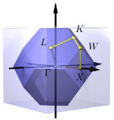
Figure 11: (Color online) Magnetic Brillouin zone of the simple cubic lattice and the path along high symmetry points used for the presentation of spectra in the antiferromagnetically ordered state in Fig. 14

.

In order to explicitly break the full translational symmetry along with the SU(2) symmetry, we add a staggered magnetic field $h_{i}=h_{0}\,{\rm e}^{{\rm i}{\boldsymbol{Q}}\cdot{\boldsymbol{r}_{i}}}$ with ${\boldsymbol{Q}}=(\pi,\pi,\pi)$ to the Hamiltonian of Eq. (I) as

$$H_{h}=H+\sum\limits_{i}h_{i}m_{i}\;,$$ (22)

where $m_{i}=n_{i,\uparrow}-n_{i,\downarrow}$ is the spin polarization at lattice site $i$. In principle this allows the study of properties as functions of this staggered field. However, because such a field is of little experimental relevance, one is conventionally only interested in the limit $h_{0}\to 0$. If in this limit a non-zero polarization remains, we have found a state with spontaneous symmetry breaking.

In the actual simulation we add a small field and explicitly break the symmetry (in our case we chose $h_{0}=0.01$) in the initialization of our iteration process. The field is switched off after the first few iterations and the system is allowed to evolve freely. Eventually, the process converges to a solution with either a vanishing staggered magnetization $M_{i}(T)\propto\langle m_{i}\rangle\,=\,{\rm e}^{{\rm i}{\boldsymbol{Q}}\cdot{{\boldsymbol{r}}_{i}}}\,m_{s}(T)=0$, indicating a parameter regime where the thermodynamically stable state is paramagnetic, or $M_{i}\neq 0$ and thus an antiferromagnetically ordered state.

To be able to include such a field in our simulations, we have to ensure that the cluster we use has the proper translational symmetry with respect to a double unit cell. These clusters are also referred to as bipartite clusters. We again employ the systematic classification by Betts Betts and Stewart (1997) to find the optimal cluster of this type with 18 sites. Since the DCA is formulated in momentum space, the broken translational symmetry introduces explicit non-diagonal elements in quantities like the Green’s function or the self-energy. For the following we will adopt the notation

$$G_{\sigma{\boldsymbol{K}_{1}},{\boldsymbol{K}_{2}}}({\rm i}\omega_{n})=\\ \frac{1}{N}\sum\limits_{ij}\exp\left[{\rm i}\left({\boldsymbol{K}}_{1}\cdot{\boldsymbol{R}}_{i}-{\boldsymbol{K}}_{2}\cdot{\boldsymbol{R}}_{j}\right)\right]G_{\sigma ij}({\rm i}\omega_{n})$$ (23)

as extension of Eq. (5) for Green’s functions with momenta ${\boldsymbol{K}}_{1}\neq{\boldsymbol{K}}_{2}$. With this notation, Green’s function in the antiferromagnetic phase can be represented by the 2$\times$2 matrix

$${\bf G}_{\sigma{\boldsymbol{K}}^{\prime}}({\rm i}\omega_{n}):=\left(\begin{array}[]{ll}G^{00}_{\sigma\boldsymbol{K}^{\prime}}({\rm i}\omega_{n})&G^{01}_{\sigma\boldsymbol{K}^{\prime}}({\rm i}\omega_{n})\\ G^{10}_{\sigma\boldsymbol{K}^{\prime}}({\rm i}\omega_{n})&G^{11}_{\sigma\boldsymbol{K}^{\prime}}({\rm i}\omega_{n})\end{array}\right)\\ :=\begin{pmatrix}G_{\sigma{\boldsymbol{K}^{\prime}},{\boldsymbol{K}^{\prime}}}({\rm i}\omega_{n})&G_{\sigma{\boldsymbol{K}^{\prime}},{\boldsymbol{K}^{\prime}}+{\boldsymbol{Q}}}({\rm i}\omega_{n})\\ G_{\sigma{\boldsymbol{K}^{\prime}},{\boldsymbol{K}^{\prime}}+{\boldsymbol{Q}}}({\rm i}\omega_{n})&G_{\sigma{\boldsymbol{K}^{\prime}}+{\boldsymbol{Q}},{\boldsymbol{K}^{\prime}}+{\boldsymbol{Q}}}({\rm i}\omega_{n})\end{pmatrix}$$ (24)

where ${\boldsymbol{K}}^{\prime}$ is an element of the MBZ. The symmetry relations $G^{00}_{\sigma\boldsymbol{K}^{\prime}}({\rm i}\omega_{n})=G^{11}_{\bar{\sigma}\boldsymbol{K}^{\prime}}({\rm i}\omega_{n})=-\left(G^{11}_{\sigma\boldsymbol{K}^{\prime}}({\rm i}\omega_{n})\right)^{*}=-\left(G^{00}_{\bar{\sigma}\boldsymbol{K}^{\prime}}({\rm i}\omega_{n})\right)^{*}$ and $G^{10}_{\sigma\boldsymbol{K}^{\prime}}({\rm i}\omega_{n})=G^{01}_{\sigma\boldsymbol{K}^{\prime}}({\rm i}\omega_{n})=G^{10}_{\bar{\sigma}\boldsymbol{K}^{\prime}}({\rm i}\omega_{n})=G^{01}_{\bar{\sigma}\boldsymbol{K}^{\prime}}({\rm i}\omega_{n})$ hold for Green’s function as well as for the self-energy. The latter is still defined via Dyson’s equation

$${\bf\Sigma}_{\sigma\boldsymbol{K}^{\prime}}({\rm i}\omega_{n})={\boldsymbol{\cal G}}_{\sigma\boldsymbol{K}^{\prime}}({\rm i}\omega_{n})^{-1}-{\bf G}_{\sigma\boldsymbol{K}^{\prime}}({\rm i}\omega_{n})^{-1}\;.$$ (25)

which, however, now involves quantities which are $2\times 2$ matrices.

This matrix structure makes it necessary to adapt the CT-QMC algorithm accordingly. This can most conveniently be done using a spinor representation for the field operators, and rewriting the formulas with these new composite operators. A detailed account of this procedure will be given elsewhere. Here we just want to note that one can again perform measurements in Matsubara space directly and thus obtain an accurate estimate of the self-energy, which can then be analytically continued as before.

A first simple test of the method is to calculate the staggered moment

$$m_{s}=\sum\limits_{i}m_{i}\,\exp\left({{\rm i}{\boldsymbol{Q}}\cdot{\boldsymbol{r}}_{i}}\right)$$ (26)

and thus locate the antiferromagnetic phase. The results of such a calculation for $U=0.67\,W$ as function of temperature are shown in Fig. 12

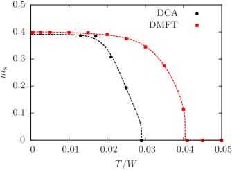
Figure 12: (Color online) Staggered magnetization $m_{s}(T)$ as function of $T$ for $U=0.67W$ as obtained from a DCA calculation with $N=18$ (circles) and the DMFT (squares). Dashed lines: guide to the eye.

for DCA simulations (circles) and, for comparison, DMFT calculations using Wilson’s numerical renormalization group algorithm as the impurity solverBulla et al. (2008) (squares). The first thing to note is that within DCA the critical temperature is reduced by roughly 30% as compared to the DMFT. The values of $T_{N}\approx 0.03\,W$ for DCA and $T_{N}\approx 0.042\,W$ for DMFT nicely agree with the results obtained by Kent et al.Kent et al. (2005a). This is in agreement with the expectation, that for a three-dimensional system far enough away from the critical region one should not see dramatic influence by the order parameter fluctuations any more. Note, however, that $m_{s}(0)\approx 0.39$ for both DMFT and DCA is reduced as compared to the Hartree approximation, where $m_{s}H(0)\approx 0.426$. Finally, while the functional shape of $m_{s}(T)$ for the DMFT nicely follows the standard mean-field behavior $m_{s}(T\nearrow T_{N})\propto\sqrt{1-T/T_{N}}$ and, respectively, $m_{s}(T\to 0)\propto 1-2{\rm e}^{-2T_{N}/T}$, the form obtained from DCA is very different, rather exhibiting a linear behavior just below $T_{N}$ and a constant value for $T\lesssim 0.02\,W$.

With the ability to perform reliable calculations in the symmetry-broken phase, one is of course interested in extracting dynamics from the simulations, preferably by analytically continuing the single-particle self-energy. To this end we again need the high-frequency behavior of the self-energy, which can be obtained from a high-frequency expansion (see the AppendixA) as

$${\bf\Sigma}_{\sigma\boldsymbol{K}^{\prime}}({\rm i}\omega_{n})=\mathord{\mathcal{O}}(({\rm i}\omega_{n})^{-2})+U\begin{pmatrix}\langle n_{\bar{\sigma}}\rangle-\frac{1}{2}&\langle m_{\bar{\sigma}}\rangle\\ \langle m_{\bar{\sigma}}\rangle&\langle n_{\bar{\sigma}}\rangle-\frac{1}{2}\\ \end{pmatrix}+\frac{U^{2}}{{\rm i}\omega_{n}}\begin{pmatrix}\langle n_{\bar{\sigma}}\rangle\left(1-\langle n_{\bar{\sigma}}\rangle\right)+\langle m_{\bar{\sigma}}\rangle^{2}&\langle m_{\bar{\sigma}}\rangle\left(1-2\langle n_{\bar{\sigma}}\rangle\right)\\ \langle m_{\bar{\sigma}}\rangle\left(1-2\langle n_{\bar{\sigma}}\rangle\right)&\langle n_{\bar{\sigma}}\rangle\left(1-\langle n_{\bar{\sigma}}\rangle\right)+\langle m_{\bar{\sigma}}\rangle^{2}\end{pmatrix}$$ (27)

using the staggered spin polarization

$$\langle m_{\sigma}\rangle=\sum\limits_{i}{\rm e}^{{\rm i}{\boldsymbol{Q}}\cdot{\boldsymbol{r}}_{i}}\langle n_{\sigma i}-n_{\bar{\sigma}i}\rangle\;.$$ (28)

The direct analytic continuation of non-diagonal self-energies—or Green’s functions—is not possible, since the non-diagonal spectral function $-\frac{1}{\pi}\text{Im}\,\Sigma^{10}_{\sigma\boldsymbol{K}^{\prime}}(\omega)$ has both negative and positive values while the standard MEM algorithm can only deal with non-negative spectral functions. In order to solve this problem, we employ the linear transformation Tomczak (2007) (omitting spin and frequency dependencies)

$$\Sigma^{\pm}_{\boldsymbol{K}^{\prime}}=\frac{\Sigma^{00}_{\boldsymbol{K}^{\prime}}+\Sigma^{11}_{\boldsymbol{K}^{\prime}}}{2}\pm\Sigma^{10}_{\boldsymbol{K}^{\prime}}$$ (29)

and determine $\text{Im}\,\Sigma^{\pm}_{\sigma\boldsymbol{K}^{\prime}}(\omega)$ along with the diagonal elements $\text{Im}\,\Sigma^{00}_{\sigma\boldsymbol{K}^{\prime}}(\omega)$ and $\text{Im}\,\Sigma^{11}_{\sigma\boldsymbol{K}^{\prime}}(\omega)$ using the MEM. As in the paramagnetic case, the high-frequency coefficients of Eq. (27) are used to normalize the self-energies prior to the analytic continuation. Finally, the real parts are calculated by a Kramers-Kronig relation analogous to Eq. (16). Since the transformation (29) is linear, it holds for the analytically continued functions as well and can thus be solved for the non-diagonal element $\Sigma^{10}_{\sigma K^{\prime}}(\omega)$. An example for a complete self-energy matrix on the real frequency axis obtained by this procedure is shown in Fig. 13.

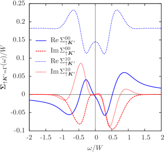
Figure 13: (Color online) Self-energy for ${\boldsymbol{K}}^{\prime}=\Gamma$, $U=0.5\,W$, $t^{\prime}=0$, and $T=0.02\,W$ in the antiferromagnetic phase. The real and imaginary parts of the elements $\Sigma^{00}_{\uparrow\boldsymbol{K}^{\prime}}(\omega)=\Sigma^{11}_{\downarrow\boldsymbol{K}^{\prime}}(\omega)=\Sigma^{11}_{\uparrow\boldsymbol{K}^{\prime}}(-\omega)=\Sigma^{00}_{\downarrow\boldsymbol{K}^{\prime}}(-\omega)$ and $\Sigma^{10}_{\uparrow\boldsymbol{K}^{\prime}}(\omega)=\Sigma^{01}_{\uparrow\boldsymbol{K}^{\prime}}(\omega)=\Sigma^{10}_{\downarrow\boldsymbol{K}^{\prime}}(\omega)=\Sigma^{01}_{\downarrow\boldsymbol{K}^{\prime}}(\omega)$ are shown.

Note that the diagonal and off-diagonal elements have different symmetry properties. For the particle-hole symmetric situation presented here, the former obey the relation $\Sigma^{\alpha\alpha}_{\sigma\boldsymbol{K}^{\prime}}(\omega+i0^{+})=\Sigma^{\alpha\alpha}_{\bar{\sigma}\boldsymbol{K}^{\prime}}(-\omega+i0^{+})$ and, respectively, $\Sigma^{\bar{\alpha}\bar{\alpha}}_{\sigma\boldsymbol{K}^{\prime}}(\omega+i0^{+})=\Sigma^{\alpha\alpha}_{\sigma\boldsymbol{K}^{\prime}}(-\omega+i0^{+})$ following from the structure of the Néel state, while the latter are all identical but obey $\Sigma^{\alpha\bar{\alpha}}_{\sigma\boldsymbol{K}^{\prime}}(\omega+i0^{+})=-\Sigma^{\alpha\bar{\alpha}}_{\bar{\sigma}\boldsymbol{K}^{\prime}}(-\omega+i0^{+})$. This last relation in particular implies that the real part is an even function of $\omega$, and the imaginary part is odd.

The resulting self-energies for the cluster $\boldsymbol{K}^{\prime}$ points are then interpolated as in the paramagnetic case, and finally the spin-averaged spectral function for all momenta $\boldsymbol{k}^{\prime}$ of the magnetic Brillouin zone follows from

$$A_{\boldsymbol{k}^{\prime}}(\omega)=-\frac{1}{\pi}\text{Im}\,\text{Tr}\,\\ \left[\left(\begin{array}[]{l}\omega+\mu-\epsilon_{\boldsymbol{k}^{\prime}}\qquad\ \ 0\\ 0\hfill\omega+\mu-\epsilon_{{\boldsymbol{k}}^{\prime}+{\boldsymbol{Q}}}\end{array}\right)-{\bf\Sigma}_{{\boldsymbol{k}}^{\prime}}(\omega)\right]^{-1}\;,$$ (30)

where Tr denotes the trace over the 2$\times$2-matrix.

Results for single-particle spectra in the antiferromagnetically ordered phase and different values of $U$ for $T=0.02\,W$ are shown in Figs. 14(a)–14(c)

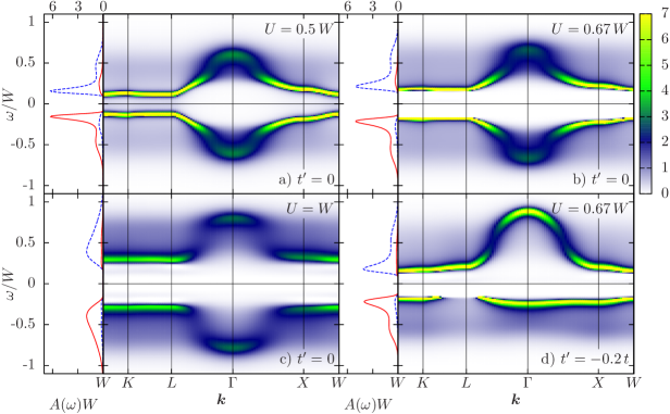
Figure 14: (Color online) Spin-averaged single-particle spectra for $T=0.02\,W$ in the antiferromagnetic phase for different interaction strengths. Panel (d) shows a spectrum for non-zero next-nearest-neighbor hopping $t^{\prime}=-0.2\,t$. The left part of each figure depicts the local single-particle spectrum for both the majority spins (full red line) and the minority spins (dashed blue line). In (a) the edges of the gap are too sharp to resolve properly. To avoid a numerical division by zero, an artificial imaginary shift $-{\rm i}\delta$ with $\delta=0.03\,W$ was added to the self-energy. The result is a slight broadening of the gap edges. The interpolation follows the path along the high symmetry points of the reduced Brillouin zone depicted in Fig. 13(b).

for paths connecting high symmetry points in the magnetic Brillouin zone in Fig. 13(b). As expected, the spectral function and DOS have a gap around the Fermi energy, i. e., we always have an insulating state. Furthermore, it is symmetric with respect to the Fermi energy, reflecting the back-folding of the spectrum due to the broken translational symmetry. Along a large part of the Brillouin zone one has rather flat bands. For weak and moderate coupling these structures have a rather high spectral weight, which results in the formation of characteristic van Hove singularities at the gap edges. This is a typical weak-coupling result consistent with a conventional Hartree approximation. The gap increases for increasing $U$, while at the same time the weight in the structures at the gap edges is redistributed to larger energies, leading to a softening of the structures in the DOS.

Figure 14(d) shows an antiferromagnetic spectrum for non-zero $t^{\prime}=-0.2\,t$. The next-nearest-neighbor hopping breaks the symmetry with respect to the Fermi energy analogous to the paramagnetic case. Since magnetically frustrating interactions cause the antiferromagnetic phase to quickly vanish at the present temperature, no larger value of $t^{\prime}$ was simulated.

V Conclusion

The dynamical-cluster approximation is a controlled, systematically improvable approach to the solution of strongly correlated electronic model systems. Due to the size and complexity of the cluster impurity problem, only quantum Monte Carlo methods are available as efficient and unbiased quantum impurity solver algorithms. While they yield in principle arbitrarily accurate imaginary-frequency data, extracting spectral functions from QMC data is an ill-posed numerical problem and hence remains a difficult task. It requires an analytical continuation based on maximum entropy or a similar procedure and a thorough error analysis for the quantity to be continued including analytically supplemented high-frequency information. The previously used Hirsch-Fye QMC impurity solver algorithm made the direct continuation of the irreducible self-energy prohibitively expensive and made comparatively unreliable root-searching techniques necessary.

The advent of modern continuous-time Monte-Carlo algorithms allows a direct simulation of data in frequency space and moreover yields high-quality data for the self-energy with reliable error estimates, thus allowing a direct analytical continuation of the self-energy.

Based on this new route we presented a method to extract momentum-resolved dynamical correlation functions from QMC simulations of strongly correlated electron systems. We showed that QMC simulation of clusters within the dynamical cluster approximation can provide data accurate enough to enable the calculation of both momentum- and frequency-resolved single-particle spectra. The method can resolve detailed structures in the spectral functions, including waterfall-like features. We observe that even in three dimensions, momentum resolved self-energies lead to spectra that are qualitatively different from dynamical mean-field spectra, and present a more reliable starting point for an extrapolation to the lattice system.

In addition we showed that we can access momentum- and frequency-resolved spectra in the paramagnetic state as well as in more complex ordered phases. As an example we discussed spectral properties of the Hubbard model inside the antiferromagnetic phase, also including an additional magnetic frustration introduced by a next-nearest neighbor hopping.

We detected the interaction driven metal-insulator transition at $T=0.012\,W_{\mathrm{eff}}$ and $U_{\mathrm{c}}=0.94(3)\,W_{\mathrm{eff}}$, a value which is substantially smaller than the DMFT result $U_{\mathrm{c}}=1.18(2)\,W_{\mathrm{eff}}$. For non-zero values of $t^{\prime}$ no MH-MIT could be detected for temperatures $T\geq 0.01\,W$. The presence of a smooth cross-over indicates that the transition has moved to lower temperatures—an effect, that that has been previously studied within the context of DMFT.Peters and Pruschke (2009b) To clarify this point as well as the $t^{\prime}$ dependence of $U_{\mathrm{c}}$ further studies at lower temperatures are necessary. Furthermore, in contrast to the standard expectation, the MH-MIT appears not to be purely local, but rather occurs initially for $\boldsymbol{k}$ points at the Fermi surface only. This $\boldsymbol{k}$-dependent behavior is different from the momentum-selective Mott transition found for the two-dimensional Hubbard modelFerrero et al. (2009c) where the Mott transition occurs only on selected parts of the Fermi surface. We do not observe such a behavior in our data, but for a definite statement on this issue calculations on larger clusters would be required.

Appendix A High-frequency expansion of the self-energies

We extend the results obtained for the dynamical mean field theory Potthoff et al. (1997); Comanac (2007) to the momentum-dependent case encountered in the DCA, both for the paramagnetic and the antiferromagnetic phase.

The antiferromagnetic coarse-grained Green’s function $\bar{\bf G}_{\sigma\boldsymbol{K}^{\prime}}({\rm i}\omega_{n})$ in the presence of a staggered magnetic field can be described by Maier et al. (2005a)

$$\bar{\bf G}_{\sigma\boldsymbol{K}^{\prime}}({\rm i}\omega_{n})=\frac{1}{V}\int\!{{\rm d}}\tilde{\boldsymbol{k}}\\ \left[\left(\begin{array}[]{l}{\rm i}\omega_{n}-\xi_{{\boldsymbol{K}^{\prime}}+\tilde{\boldsymbol{k}}}\qquad\ \ h_{\sigma}/2\\ h_{\sigma}/2\hfill{\rm i}\omega_{n}-\xi_{{\boldsymbol{K}}^{\prime}+{\boldsymbol{Q}}+\tilde{\boldsymbol{k}}}\end{array}\right)-{\bf\Sigma}_{\boldsymbol{K}^{\prime}}({\rm i}\omega_{n})\right]^{-1}\;$$ (31)

using the matrix notation of Eq. (24) and $\xi_{\boldsymbol{K}^{\prime}}=\epsilon_{\boldsymbol{K}^{\prime}}-\mu$. To gain an expression for the high-frequency coefficients of the self-energy, we use the ansatz

$${\bf\Sigma}_{\sigma\bf K^{\prime}}({\rm i}\omega_{n})={\bf\Sigma}^{0}_{\sigma\boldsymbol{K}^{\prime}}+\frac{{\bf\Sigma}^{1}_{\sigma\boldsymbol{K}^{\prime}}}{{\rm i}\omega_{n}}+\mathord{\mathcal{O}}\left(({\rm i}\omega_{n})^{-2}\right)\;$$ (32)

and expand the coarse-grained Green’s function up to third order:

$$\bar{\bf G}_{\sigma\boldsymbol{K}^{\prime}}({\rm i}\omega_{n})=\frac{{\bf C}^{1}_{\sigma\boldsymbol{K}^{\prime}}}{{\rm i}\omega_{n}}+\frac{{\bf C}^{2}_{\sigma\boldsymbol{K}^{\prime}}}{\left({\rm i}\omega_{n}\right)^{2}}+\frac{{\bf C}^{3}_{\sigma\boldsymbol{K}^{\prime}}}{\left({\rm i}\omega_{n}\right)^{3}}+\mathord{\mathcal{O}}\left(({\rm i}\omega_{n})^{-4}\right)\;.$$ (33)

The result is

$${\bf C}^{1}_{\sigma\boldsymbol{K}^{\prime}}= \begin{pmatrix}1&0\\ 0&1\end{pmatrix}\;,$$ (34)

$${\bf C}^{2}_{\sigma\boldsymbol{K}^{\prime}}= \begin{pmatrix}\overline{\xi}_{\boldsymbol{K}^{\prime}}&h_{\sigma}/2\\ h_{\sigma}/2&\overline{\xi}_{{\boldsymbol{K}^{\prime}}+{\boldsymbol{Q}}}\\ \end{pmatrix}+{\bf\Sigma}^{0}_{\sigma\boldsymbol{K}^{\prime}}\;,$$ (35)

$${\bf C}^{3}_{\sigma\boldsymbol{K}^{\prime}}= \overline{\left[\begin{pmatrix}\xi_{\boldsymbol{K}^{\prime}}&h_{\sigma}/2\\ h_{\sigma}/2&\xi_{{\boldsymbol{K}^{\prime}}+{\boldsymbol{Q}}}\\ \end{pmatrix}+{\bf\Sigma}^{0}_{\sigma\boldsymbol{K}^{\prime}}\right]^{2}}+{\bf\Sigma}^{1}_{\sigma\boldsymbol{K}^{\prime}}\;,$$ (36)

where the over-lined quantities are coarse grained over the momentum patch centered around $\boldsymbol{K}^{\prime}$, e. g.

$$\overline{\xi}_{\boldsymbol{K}^{\prime}}=\frac{1}{V}\int\!{\rm d}\tilde{\boldsymbol{k}}\,\xi_{{\boldsymbol{K}^{\prime}}+\tilde{\boldsymbol{k}}}\;.$$ (37)

A direct calculation of the Green’s function using Heisenberg’s equations of motion provides the information necessary for the determination of the unknown coefficients ${\bf\Sigma}^{0}_{\sigma\boldsymbol{K}^{\prime}}$ and ${\bf\Sigma}^{1}_{\sigma\boldsymbol{K}^{\prime}}$. Starting again with the Hamiltonian (22), the high frequency coefficients of the single-particle Green’s function in real space

$$G_{\sigma ij}({\rm i}\omega_{n})=\frac{C^{1}_{\sigma ij}}{{\rm i}\omega_{n}}+\frac{C^{2}_{\sigma ij}}{\left({\rm i}\omega_{n}\right)^{2}}+\frac{C^{3}_{\sigma ij}}{\left({\rm i}\omega_{n}\right)^{3}}+\mathord{\mathcal{O}}\left(({\rm i}\omega_{n})^{-4}\right)$$ (38)

can be obtained Comanac (2007) via

$$C^{1}_{\sigma ij}= \left\langle\left\{c_{\sigma i},c^{\dagger}_{\sigma j}\right\}\right\rangle\;,$$ (39)

$$C^{2}_{\sigma ij}= -\left\langle\left\{\left[H_{h},c_{\sigma i}\right],c^{\dagger}_{\sigma j}\right\}\right\rangle\;,$$ (40)

$$C^{3}_{\sigma ij}= \left\langle\left\{\left[H_{h},\left[H_{h},c_{\sigma i}\right]\right],c^{\dagger}_{\sigma j}\right\}\right\rangle\;.$$ (41)

Here $[A,B]$ ($\{A,B\}$) denotes the (anti)commutator of the operators $A$ and $B$. A straightforward calculation yields

$$C^{1}_{\sigma ij} =\delta_{ij}\;,$$ (42)

$$C^{2}_{\sigma ij} =-\tilde{\xi}_{ij}-\left[h_{\sigma i}+U\langle n_{\bar{\sigma}i}\rangle\right]\delta_{ij}\;,$$ (43)

$$C^{3}_{\sigma ij} =\sum\limits_{m}\tilde{\xi}_{im}\tilde{\xi}_{mj}+\left(h_{\sigma i}h_{\sigma j}+U^{2}\langle n_{\bar{\sigma}i}\rangle\right)\delta_{ij}$$

$$-\left(h_{\sigma i}+h_{\sigma j}\right)\tilde{\xi}_{ij}$$

$$-U\left(n_{\bar{\sigma}i}+n_{\bar{\sigma}j}\right)\left(\tilde{\xi}_{ij}-h_{\sigma i}\delta_{ij}\right)\;,$$ (44)

where $\tilde{\xi}_{ij}=t+\left(\mu+\frac{U}{2}\right)\delta_{ij}$ for nearest neighbors, $\tilde{\xi}_{ij}=t^{\prime}+\left(\mu+\frac{U}{2}\right)\delta_{ij}$ for next-nearest neighbors, and zero otherwise. The high frequency coefficients of the coarse-grained Green’s function in cluster momentum space [Eq. (33)] are readily calculated by a Fourier transformation of Eqs. (42)–(44) followed by a coarse-graining in ${\boldsymbol{k}}$-space. One obtains

$${\bf C}^{1}_{\sigma\boldsymbol{K}^{\prime}}= \begin{pmatrix}1&0\\ 0&1\end{pmatrix}$$ (45)

$${\bf C}^{2}_{\sigma\boldsymbol{K}^{\prime}}= \begin{pmatrix}\overline{\tilde{\xi}}_{\boldsymbol{K}^{\prime}}+U\langle n_{\bar{\sigma}}\rangle&U\langle m_{\bar{\sigma}}\rangle+h_{\sigma}/2\\ U\langle m_{\bar{\sigma}}\rangle+h_{\sigma}/2&\overline{\tilde{\xi}}_{{\boldsymbol{K}^{\prime}}+{\boldsymbol{Q}}}+U\langle n_{\bar{\sigma}}\rangle\\ \end{pmatrix}$$ (46)

$${\bf C}^{3}_{\sigma\boldsymbol{K}^{\prime}}=\left(\begin{array}[]{l}\overline{\tilde{\xi}^{2}}_{\boldsymbol{K}^{\prime}}+h_{\sigma}^{2}/4+2U\langle n_{\bar{\sigma}}\rangle\overline{\tilde{\xi}}_{\boldsymbol{K}^{\prime}}+U^{2}\langle n_{\bar{\sigma}}\rangle+Uh_{\sigma}\langle m_{\bar{\sigma}}\rangle\\ \left(U\langle m_{\bar{\sigma}}\rangle+h_{\sigma}/2\right)\left(\overline{\tilde{\xi}}_{\boldsymbol{K}^{\prime}}+\overline{\tilde{\xi}}_{{\boldsymbol{K}^{\prime}}+{\boldsymbol{Q}}}\right)+U^{2}\langle m_{\bar{\sigma}}\rangle+Uh_{\sigma}\langle n_{\bar{\sigma}}\rangle\end{array}\right.\\ \left.\begin{array}[]{r}\left(U\langle m_{\bar{\sigma}}\rangle+h_{\sigma}/2\right)\left(\overline{\tilde{\xi}}_{\boldsymbol{K}^{\prime}}+\overline{\tilde{\xi}}_{{\boldsymbol{K}^{\prime}}+{\boldsymbol{Q}}}\right)+U^{2}\langle m_{\bar{\sigma}}\rangle+Uh_{\sigma}\langle n_{\bar{\sigma}}\rangle\\ \overline{\tilde{\xi}^{2}}_{{\boldsymbol{K}^{\prime}}+{\boldsymbol{Q}}}+h_{\sigma}^{2}/4+2U\langle n_{\bar{\sigma}}\rangle\overline{\tilde{\xi}}_{{\boldsymbol{K}^{\prime}}+{\boldsymbol{Q}}}+U^{2}\langle n_{\bar{\sigma}}\rangle+Uh_{\sigma}\langle m_{\bar{\sigma}}\rangle\end{array}\right)\;,$$ (47)

where $\tilde{\xi}_{\boldsymbol{K}^{\prime}}=\xi_{\boldsymbol{K}^{\prime}}-U/2$ and

$$\langle m_{\sigma}\rangle=\sum\limits_{i}{\rm e}^{{\rm i}{\boldsymbol{Q}}\cdot{\boldsymbol{r}}_{i}}\langle n_{\sigma i}-n_{\bar{\sigma}i}\rangle\;.$$ (48)

A comparison with Eqs. 34–36 yields

$${\bf\Sigma}^{0}_{\boldsymbol{K}^{\prime}}=U\begin{pmatrix}\langle n_{\bar{\sigma}}\rangle-\frac{1}{2}&\langle m_{\bar{\sigma}}\rangle\\ \langle m_{\bar{\sigma}}\rangle&\langle n_{\bar{\sigma}}\rangle-\frac{1}{2}\\ \end{pmatrix}$$ (49)

$${\bf\Sigma}^{1}_{\boldsymbol{K}^{\prime}}=U^{2}\left(\begin{array}[]{l}\langle n_{\bar{\sigma}}\rangle\left(1-\langle n_{\bar{\sigma}}\rangle\right)+\langle m_{\bar{\sigma}}\rangle^{2}\\ \langle m_{\bar{\sigma}}\rangle\left(1-2\langle n_{\bar{\sigma}}\rangle\right)\\ \end{array}\right.\\ \left.\begin{array}[]{l}\langle m_{\bar{\sigma}}\rangle\left(1-2\langle n_{\bar{\sigma}}\rangle\right)\\ \langle n_{\bar{\sigma}}\rangle\left(1-\langle n_{\bar{\sigma}}\rangle\right)+\langle m_{\bar{\sigma}}\rangle^{2}\end{array}\right)\;,$$ (50)

which is the solution shown in Eq. 27. The non-diagonal parts vanish for $\langle m_{\sigma}\rangle=0$ and the expression simplifies to the paramagnetic solution of Eqs. (11) and (12).

References

- Hubbard (1963) J. Hubbard, Proc. Roy. Soc. London A 276, 238 (1963).
- Gutzwiller (1963) M. C. Gutzwiller, Phys. Rev. Lett. 10, 159 (1963).
- Kanamori (1963) J. Kanamori, Prog. Theor. Phys. 30, 275 (1963).
- Essler et al. (2005) F. H. Essler, H. Frahm, F. Göhmann, A. Klümper, and V. E. Korepin, The One-Dimensional Hubbard Model (Cambridge University Press, 2005).
- Georges et al. (1996) A. Georges, G. Kotliar, W. Krauth, and M. J. Rozenberg, Rev. Mod. Phys. 68, 13 (1996).
- Fulde (1991) P. Fulde, Electron Correlations in Molecules and Solids, Springer Series in Solid-State Sciences (Springer Verlag, Berlin/Heidelberg/New York, 1991).
- Troyer and Wiese (2005) M. Troyer and U.-J. Wiese, Phys. Rev. Lett. 94, 170201 (2005).
- Kotliar et al. (2006) G. Kotliar, S. Y. Savrasov, K. Haule, V. S. Oudovenko, O. Parcollet, and C. A. Marianetti, Rev. Mod. Phys. 78, 865 (2006).
- Maier et al. (2005a) T. Maier, M. Jarrell, T. Pruschke, and M. H. Hettler, Rev. Mod. Phys. 77, 1027 (2005a).
- Fuchs et al. (2011) S. Fuchs, E. Gull, L. Pollet, E. Burovski, E. Kozik, T. Pruschke, and M. Troyer, Phys. Rev. Lett. 106, 030401 (2011).
- Gull et al. (2011a) E. Gull, P. Staar, S. Fuchs, P. Nukala, M. S. Summers, T. Pruschke, T. C. Schulthess, and T. Maier, Phys. Rev. B 83, 075122 (2011a).
- Pruschke and Zitzler (2003) T. Pruschke and R. Zitzler, J. Phys.: Condens. Matter 15, 7867 (2003).
- Peters and Pruschke (2009a) R. Peters and T. Pruschke, New J. Phys. 11, 083022 (2009a).
- Koch et al. (2008) E. Koch, G. Sangiovanni, and O. Gunnarsson, Phys. Rev. B 78, 115102 (2008).
- Dagotto (1994) E. Dagotto, Rev. Mod. Phys. 66, 763 (1994).
- Moukouri and Jarrell (2001) S. Moukouri and M. Jarrell, Phys. Rev. Lett. 87, 167010 (2001).
- Onoda and Imada (2003) S. Onoda and M. Imada, Phys. Rev. B 67, 161102 (2003).
- Parcollet et al. (2004) O. Parcollet, G. Biroli, and G. Kotliar, Phys. Rev. Lett. 92, 226402 (2004).
- Hanasaki and Imada (2006) K. Hanasaki and M. Imada, Journal of the Physical Society of Japan 75, 084702 (2006).
- Zhang and Imada (2007) Y. Z. Zhang and M. Imada, Phys. Rev. B 76, 045108 (2007).
- Liebsch et al. (2008) A. Liebsch, H. Ishida, and J. Merino, Phys. Rev. B 78, 165123 (2008).
- Gull et al. (2008a) E. Gull, P. Werner, X. Wang, M. Troyer, and A. J. Millis, EPL (Europhysics Letters) 84, 37009 (2008a).
- Park et al. (2008) H. Park, K. Haule, and G. Kotliar, Phys. Rev. Lett. 101, 186403 (2008).
- Gull et al. (2009) E. Gull, O. Parcollet, P. Werner, and A. J. Millis, Phys. Rev. B 80, 245102 (2009).
- Werner et al. (2009) P. Werner, E. Gull, O. Parcollet, and A. J. Millis, Phys. Rev. B 80, 045120 (2009).
- De Leo et al. (2011) L. De Leo, J.-S. Bernier, C. Kollath, A. Georges, and V. W. Scarola, Phys. Rev. A 83, 023606 (2011).
- Kent et al. (2005a) P. R. C. Kent, M. Jarrell, T. A. Maier, and T. Pruschke, Phys. Rev. B 72, 060411 (2005a).
- Hettler et al. (1998) M. H. Hettler, A. N. Tahvildar-Zadeh, M. Jarrell, T. Pruschke, and H. R. Krishnamurthy, Phys. Rev. B 58, R7475 (1998).
- Maier et al. (2005b) T. A. Maier, M. Jarrell, T. C. Schulthess, P. R. C. Kent, and J. B. White, Phys. Rev. Lett. 95, 237001 (2005b).
- Jarrell and Gubernatis (1996) M. Jarrell and J. Gubernatis, Phys. Rep. 269, 133 (1996).
- Hirsch and Fye (1986) J. E. Hirsch and R. M. Fye, Phys. Rev. Lett. 56, 2521 (1986).
- Rubtsov and Lichtenstein (2004) A. N. Rubtsov and A. I. Lichtenstein, JETP Lett. 80, 61 (2004).
- Rubtsov et al. (2005) A. N. Rubtsov, V. V. Savkin, and A. I. Lichtenstein, Phys. Rev. B 72, 035122 (2005).
- Gull et al. (2008b) E. Gull, P. Werner, O. Parcollet, and M. Troyer, EPL (Europhysics Letters) 82, 57003 (2008b).
- Werner et al. (2006) P. Werner, A. Comanac, L. de’ Medici, M. Troyer, and A. J. Millis, Phys. Rev. Lett. 97, 076405 (2006).
- Gull et al. (2010) E. Gull, A. J. Millis, A. I. Lichtenstein, A. N. Rubtsov, M. Troyer, and P. Werner, ArXiv e-prints (2010), eprint 1012.4474.
- Gull et al. (2007) E. Gull, P. Werner, A. Millis, and M. Troyer, Phys. Rev. B 76, 235123 (2007).
- Wang et al. (2009) X. Wang, E. Gull, L. de’ Medici, M. Capone, and A. J. Millis, Phys. Rev. B 80, 045101 (2009).
- Jarrell et al. (1995) M. Jarrell, J. K. Freericks, and T. Pruschke, Phys. Rev. B 51, 11704 (1995).
- Miller (1974) R. G. Miller, Biometrika 61, 1 (1974).
- Bryan (1990) R. K. Bryan, Eur. Biophys. J. 18, 165 (1990).
- Akima (1970) H. Akima, J. ACM 17, 589 (1970), ISSN 0004-5411.
- Betts and Stewart (1997) D. D. Betts and G. E. Stewart, Can. J. Phys. 75, 47 (1997).
- Graf et al. (2007) J. Graf, G.-H. Gweon, K. McElroy, S. Y. Zhou, C. Jozwiak, E. Rotenberg, A. Bill, T. Sasagawa, H. Eisaki, S. Uchida, et al., Phys. Rev. Lett. 98, 067004 (2007).
- Kampf and Schrieffer (1990) A. P. Kampf and J. R. Schrieffer, Phys. Rev. B 42, 7967 (1990).
- Imada et al. (1998) M. Imada, A. Fujimori, and Y. Tokura, Rev. Mod. Phys. 70, 1039 (1998).
- R. Staudt et al. (2000) R. Staudt, M. Dzierzawa, and A. Muramatsu, Eur. Phys. J. B 17, 411 (2000).
- Moeller et al. (1995) G. Moeller, Q. Si, G. Kotliar, M. Rozenberg, and D. S. Fisher, Phys. Rev. Lett. 74, 2082 (1995).
- Kotliar et al. (2002) G. Kotliar, S. Murthy, and M. Rozenberg, Phys. Rev. Lett. 89, 046401 (2002).
- Georges et al. (2004) A. Georges, S. Florens, and T. Costi, J. de Phys. IV 114, 165 (2004).
- Ferrero et al. (2009a) M. Ferrero, P. S. Cornaglia, L. D. Leo, O. Parcollet, G. Kotliar, and A. Georges, EPL (Europhysics Letters) 85, 57009 (2009a).
- Ferrero et al. (2009b) M. Ferrero, P. S. Cornaglia, L. De Leo, O. Parcollet, G. Kotliar, and A. Georges, Phys. Rev. B 80, 064501 (2009b).
- Gull et al. (2010) E. Gull, M. Ferrero, O. Parcollet, A. Georges, and A. J. Millis, Phys. Rev. B 82, 155101 (2010).
- Lin et al. (2010) N. Lin, E. Gull, and A. J. Millis, Phys. Rev. B 82, 045104 (2010).
- Sordi et al. (2010) G. Sordi, K. Haule, and A.-M. Tremblay, Phys. Rev. Lett. 104, 226402 (2010).
- Serene and Hess (1991) J. W. Serene and D. W. Hess, Phys. Rev. B 44, 3391 (1991).
- Peters and Pruschke (2009b) R. Peters and T. Pruschke, Phys. Rev. B 79, 045108 (2009b).
- Bulla et al. (2001) R. Bulla, T. A. Costi, and D. Vollhardt, Phys. Rev. B 64, 045103 (2001).
- Joo and Oudovenko (2001) J. Joo and V. Oudovenko, Phys. Rev. B 64, 193102 (2001).
- Bulla (1999) R. Bulla, Phys. Rev. Lett. 83, 136 (1999).
- Žitko et al. (2009) R. Žitko, J. Bonča, and T. Pruschke, Phys. Rev. B 80, 245112 (2009).
- Kent et al. (2005b) P. R. C. Kent, M. Jarrell, T. A. Maier, and T. Pruschke, Phys. Rev. B 72, 060411 (2005b).
- Bulla et al. (2008) R. Bulla, T. A. Costi, and T. Pruschke, Rev. Mod. Phys. 80, 395 (2008).
- Tomczak (2007) J. M. Tomczak, Ph.D. thesis, Ecole Polytechnique, Palaiseau (2007).
- Ferrero et al. (2009c) M. Ferrero, P. S. Cornaglia, L. D. Leo, O. Parcollet, G. Kotliar, and A. Georges, EPL (Europhysics Letters) 85, 57009 (2009c), URL http://stacks.iop.org/0295-5075/85/i=5/a=57009.
- Bauer et al. (2011) B. Bauer, L. D. Carr, H. Evertz, A. Feiguin, J. Freire, S. Fuchs, L. Gamper, J. Gukelberger, E. Gull, S. Guertler, et al., Journal of Statistical Mechanics: Theory and Experiment 2011, P05001 (2011), URL http://stacks.iop.org/1742-5468/2011/i=05/a=P05001.
- Gull et al. (2011b) E. Gull, P. Werner, S. Fuchs, B. Surer, T. Pruschke, and M. Troyer, Computer Physics Communications 182, 1078 (2011b), ISSN 0010-4655.
- Potthoff et al. (1997) M. Potthoff, T. Wegner, and W. Nolting, Phys. Rev. B 55, 16132 (1997).
- Comanac (2007) A. Comanac, Ph.D. thesis, Columbia University, New York (2007).