A conservative coupling algorithm between a compressible flow and a rigid body using an Embedded Boundary method

Laurent Monasse${}^{\textrm{1, 2, 3}}$, Virginie Daru${}^{\textrm{3, 4}}$, Christian Mariotti${}^{\textrm{1}}$, Serge Piperno${}^{\textrm{2}}$, Christian Tenaud${}^{\textrm{3}}$

 

ABSTRACT

This paper deals with a new solid-fluid coupling algorithm between a rigid body and an unsteady compressible fluid flow, using an Embedded Boundary method. The coupling with a rigid body is a first step towards the coupling with a Discrete Element method. The flow is computed using a Finite Volume approach on a Cartesian grid. The expression of numerical fluxes does not affect the general coupling algorithm and we use a one-step high-order scheme proposed by Daru and Tenaud [Daru V,Tenaud C., J. Comput. Phys. 2004]. The Embedded Boundary method is used to integrate the presence of a solid boundary in the fluid. The coupling algorithm is totally explicit and ensures exact mass conservation and a balance of momentum and energy between the fluid and the solid. It is shown that the scheme preserves uniform movement of both fluid and solid and introduces no numerical boundary roughness. The efficiency of the method is demonstrated on challenging one- and two-dimensional benchmarks.

Key Words: Compressible flows; Shock capturing scheme; Discrete Element method; Fluid-structure interaction; Embedded Boundary method
 

1 Introduction

This work is devoted to the development of a coupling method for fluid-structure interaction in the compressible case. We intend to simulate transient dynamics problems, such as the impact of shock waves onto a structure, with possible fracturing causing the ultimate breaking of the structure. An inviscid fluid flow model is considered, being convenient for treating such short time scale phenomena. The simulation of fluid-structure interaction problems is often computationally challenging due to the generally different numerical methods used for solids and fluids and the instability that may occur when coupling these methods. Monolithic methods have been employed, using an Eulerian formulation for both the solid and the fluid (for instance, the diffusive interface method [16, 1]), or a Lagrangian formulation for both the fluid and the solid (for example, the PFEM method [26]), but in general, most solid solvers use Lagrangian formulations and fluid solvers use Eulerian formulations. In this paper we consider the coupling of a Lagrangian solid solver with an Eulerian fluid solver.

For the coupling in space, a possible choice is to deform the fluid domain in order to follow the movement of the solid boundary: the Arbitrary Lagrangian-Eulerian (ALE) method has been developed to that end. It has been widely used for incompressible [11, 19] and compressible [15] fluid-structure interaction. However, when solid impact or fracture occur, ALE methods are faced with a change of topology in the fluid domain that requires remeshing and projection of the fluid state on the new mesh, which are costly and error prone procedures. Moreover remeshing is poorly adapted to load balancing for parallel computations.

In order to allow for easier fracturing of the solid, we instead choose a method based on fictitious domains that solves the fluid flow on a fixed Eulerian mesh, on which a Lagrangian solid body is superimposed. A special treatment is then applied on fluid cells near the boundary and inside the solid. Different types of fictitious domain methods have been developed over the last thirty years. They can roughly be classified in three main classes: penalization methods, interpolation methods and conservative methods. Among penalization methods, the Immersed Boundary method is certainly the best known and most widely used for fluid-structure interaction. It was originally introduced by Peskin for incompressible blood flows [44, 45]. The solid boundaries deform under the action of the fluid velocity, and the presence of the solid adds forces in the fluid formulation that enforce the impermeability of the solid. However, Xu and Wang have pointed out some numerical leaking of fluid into the solid [49]. Following Leveque and Li [33, 34], they advocate the use of the Immersed Interface method, which incorporates jump conditions in the finite differences used. However, the absence of fluid mass loss is still not ensured exactly. In a different approach, Olovsson et al. [40, 2] couple an Eulerian and a Lagrangian method by penalizing the penetration of the solid into the fluid by a damped spring force. As the stiffness of the spring goes to infinity, the penetration goes to zero. Boiron et al. [5] and Paccou et al. [41] consider the solid as a porous medium, using a Brinkman porosity model. As the porosity goes to zero, the solid becomes impermeable. However, in both cases, as the stiffness grows or the porosity decreases, the use of implicit schemes is mandatory to avoid the severe stability condition of explicit schemes [5, 41]. For the high speed phenomena we consider, we use explicit solid and fluid solvers and an explicit coupling algorithm is better suited in order to avoid costly iterative procedures.

A second class of fictitious domain methods consists in enforcing the boundary conditions through interpolations in the vicinity of the boundary, using the exact values taken by the fluid on the boundary [37, 13]. The method seems to be very versatile, being used with incompressible Navier-Stokes [37, 13], Reynolds-averaged Navier-Stokes [10, 29, 30], turbulent boundary layer laws [6] and compressible Navier-Stokes [42]. The Ghost Fluid method developed by Fedkiw et al. [18, 17] relies on the same type of principle for compressible fluids. The interface is tracked using a level-set function, and conditions are applied on both sides of the interface to interpolate the boundary conditions. The advantage of these methods is that they do not suffer from additional time-step restriction due to stability, and the order of accuracy of the boundary conditions can be set a priori. However, the interpolation does not ensure the conservation of mass, momentum and energy in the system. This can cause problems when dealing with shock waves interacting with solids.

In this article, we rather consider the third class of conservative fictitious domain methods, which seems the most adequate framework to develop our coupling algorithm. These methods are generally referred to as Embedded Boundary methods, and they rely on a modified integration of the numerical fluid fluxes in the cells cut by the solid boundary [43, 14, 22, 25]. The original idea of the method can be traced back to Noh’s CEL code [39]. The new contribution of the present work consists in the coupling algorithm and its properties. The Embedded Boundary method that we use is essentially identical to previous works [43, 14, 22, 25]. The different versions of the Embedded Boundary method mainly differ in the way the stability condition arising from small cut-cells is enforced and we develop here a slightly different procedure in order to deal with solid boundaries coming close to each other. The method can be implemented independently from the time integration scheme used for the fluid, whether based on space-time splitting or multi-level time integration. Conservative fictitious domain methods have proven to give satisfactory conservation results for inviscid compressible flows in the case of static solid boundaries. Nevertheless, to our knowledge, conservation issues of the coupling have not been studied in the case of moving solids. We establish new conservation results in such a case. Our coupling method is designed to be capable of treating the general case of moving deformable bodies. In the present work, however, we only consider non-deformable (rigid) solid bodies. The case of deformable bodies is the object of ongoing work.

The fluid and solid solvers that we consider were chosen according to their ability to deal with shock waves and fracturing solids. The solid solver is based on a Discrete Element method, implemented in a code named Mka3D in the CEA [35]. It can handle elasticity as well as fracture and impact of solids. Solids are discretized into polyhedral particles, which interact through well-designed forces and torques. The particles have a rigid-body motion, and fracture is treated in a straightforward way by removing the physical cohesion between particles. The work reported in this article is a first step towards the coupling with the Mka3D code. The time integration scheme used by Mka3D (Verlet for displacement of the center of mass and RATTLE for rotation [38]) is retained for the rigid body treatment. Concerning the fluid solver, we use a Cartesian grid explicit finite volume method, based on the high-order one-step monotonicity-preserving scheme developed in [8] and space time splitting. However we emphasize that our coupling method is independent from both the Discrete Element method (as long as a solid interface is defined) and the numerical scheme used for the fluid calculation.

The article is organized as follows: we first present briefly the solid and fluid methods in section 2. In sections 3 and 4, we describe the proposed explicit coupling procedure between the fluid and the moving solid in the framework of an Embedded Boundary method. The analysis of the conservation properties of the coupling is reported in section 5, where we show that mass, momentum and energy of the solid-fluid system are exactly preserved. In section 6, we demonstrate results about the preservation on a discrete level of two solid-fluid systems in uniform movement. Finally, we illustrate the efficiency and accuracy of the method on one and two-dimensional static and dynamic benchmarks in section 7.

2 Solid and fluid discretization methods

2.1 Solid time-discretization method

We consider a non-deformable solid (rigid body). The position and velocity of the solid are given, respectively, by the position of its center of mass $\textstyle\mathbf{X}$, the rotation matrix $\mathsf{Q}$, the velocity of the center of mass $\textstyle\mathbf{V}$ and the angular momentum matrix $\mathsf{P}$. The physical characteristics of the solid are its mass $m$ and its matrix of inertia $\mathsf{R}$ which, in the inertial frame, is a diagonal matrix with the principal moments of inertia $I_{1}$, $I_{2}$ and $I_{3}$ on the diagonal. Here, we instead use the diagonal matrix $\mathsf{D}=\text{diag}(d_{1},d_{2},d_{3})$, where:

$$\forall i\in\{1,2,3\},d_{i}=\frac{I_{1}+I_{2}+I_{3}}{2}-I_{i}.$$

The angular momentum matrix $\mathsf{P}$ can be related to the usual angular velocity vector $\textstyle\mathbf{\Omega}$ by the relation $\mathsf{P}=\mathsf{D}\mathsf{j}(\mathchoice{\mbox{\boldmath$\displaystyle\mathbf{\Omega}$}}{\mbox{\boldmath$\textstyle\mathbf{\Omega}$}}{\mbox{\boldmath$\scriptstyle\mathbf{\Omega}$}}{\mbox{\boldmath$\scriptscriptstyle\mathbf{\Omega}$}})\mathsf{Q}$, where the map $\mathsf{j}:\mathbb{R}^{3}\rightarrow\mathbb{R}^{3\times 3}$ is defined such that:

$$\forall\mathchoice{\mbox{\boldmath$\displaystyle\mathbf{x}$}}{\mbox{\boldmath$\textstyle\mathbf{x}$}}{\mbox{\boldmath$\scriptstyle\mathbf{x}$}}{\mbox{\boldmath$\scriptscriptstyle\mathbf{x}$}}\in\mathbb{R}^{3},\;\forall\mathchoice{\mbox{\boldmath$\displaystyle\mathbf{y}$}}{\mbox{\boldmath$\textstyle\mathbf{y}$}}{\mbox{\boldmath$\scriptstyle\mathbf{y}$}}{\mbox{\boldmath$\scriptscriptstyle\mathbf{y}$}}\in\mathbb{R}^{3},\;\mathsf{j}(\mathchoice{\mbox{\boldmath$\displaystyle\mathbf{x}$}}{\mbox{\boldmath$\textstyle\mathbf{x}$}}{\mbox{\boldmath$\scriptstyle\mathbf{x}$}}{\mbox{\boldmath$\scriptscriptstyle\mathbf{x}$}})\cdot\mathchoice{\mbox{\boldmath$\displaystyle\mathbf{y}$}}{\mbox{\boldmath$\textstyle\mathbf{y}$}}{\mbox{\boldmath$\scriptstyle\mathbf{y}$}}{\mbox{\boldmath$\scriptscriptstyle\mathbf{y}$}}=\mathchoice{\mbox{\boldmath$\displaystyle\mathbf{x}$}}{\mbox{\boldmath$\textstyle\mathbf{x}$}}{\mbox{\boldmath$\scriptstyle\mathbf{x}$}}{\mbox{\boldmath$\scriptscriptstyle\mathbf{x}$}}\wedge\mathchoice{\mbox{\boldmath$\displaystyle\mathbf{y}$}}{\mbox{\boldmath$\textstyle\mathbf{y}$}}{\mbox{\boldmath$\scriptstyle\mathbf{y}$}}{\mbox{\boldmath$\scriptscriptstyle\mathbf{y}$}}.$$

Let us denote by $\textstyle\mathbf{F}$ and $\textstyle\mathbf{\mathcal{M}}$ the external forces and torques acting on the solid, and by $\Delta t$ the time-step. In order to preserve the energy of the solid over time integration of the movement, we choose a symplectic second-order scheme for constrained Hamiltonian systems, the RATTLE scheme [23]:

$$\mathchoice{\mbox{\boldmath$\displaystyle\mathbf{V}$}}{\mbox{\boldmath$\textstyle\mathbf{V}$}}{\mbox{\boldmath$\scriptstyle\mathbf{V}$}}{\mbox{\boldmath$\scriptscriptstyle\mathbf{V}$}}^{n+\frac{1}{2}} =\mathchoice{\mbox{\boldmath$\displaystyle\mathbf{V}$}}{\mbox{\boldmath$\textstyle\mathbf{V}$}}{\mbox{\boldmath$\scriptstyle\mathbf{V}$}}{\mbox{\boldmath$\scriptscriptstyle\mathbf{V}$}}^{n}+\frac{\Delta t}{2m}\mathchoice{\mbox{\boldmath$\displaystyle\mathbf{F}$}}{\mbox{\boldmath$\textstyle\mathbf{F}$}}{\mbox{\boldmath$\scriptstyle\mathbf{F}$}}{\mbox{\boldmath$\scriptscriptstyle\mathbf{F}$}}^{n},$$ (1)

$$\mathchoice{\mbox{\boldmath$\displaystyle\mathbf{X}$}}{\mbox{\boldmath$\textstyle\mathbf{X}$}}{\mbox{\boldmath$\scriptstyle\mathbf{X}$}}{\mbox{\boldmath$\scriptscriptstyle\mathbf{X}$}}^{n+1} =\mathchoice{\mbox{\boldmath$\displaystyle\mathbf{X}$}}{\mbox{\boldmath$\textstyle\mathbf{X}$}}{\mbox{\boldmath$\scriptstyle\mathbf{X}$}}{\mbox{\boldmath$\scriptscriptstyle\mathbf{X}$}}^{n}+\Delta t\mathchoice{\mbox{\boldmath$\displaystyle\mathbf{V}$}}{\mbox{\boldmath$\textstyle\mathbf{V}$}}{\mbox{\boldmath$\scriptstyle\mathbf{V}$}}{\mbox{\boldmath$\scriptscriptstyle\mathbf{V}$}}^{n+\frac{1}{2}},$$ (2)

$$\mathsf{P}^{n+\frac{1}{2}} =\mathsf{P}^{n}+\frac{\Delta t}{4}\mathsf{j}(\mathchoice{\mbox{\boldmath$\displaystyle\mathbf{\mathcal{M}}$}}{\mbox{\boldmath$\textstyle\mathbf{\mathcal{M}}$}}{\mbox{\boldmath$\scriptstyle\mathbf{\mathcal{M}}$}}{\mbox{\boldmath$\scriptscriptstyle\mathbf{\mathcal{M}}$}}^{n})\mathsf{Q}^{n}+\frac{\Delta t}{2}\mathsf{\Lambda}^{n}\mathsf{Q}^{n},$$ (3)

$$\mathsf{Q}^{n+1} =\mathsf{Q}^{n}+\Delta t\mathsf{P}^{n+\frac{1}{2}}\mathsf{D}^{-1},$$ (4)

$$\text{with }\mathsf{\Lambda}^{n}\text{ such that }{(\mathsf{Q}^{n+1})}^{\text{T}}\mathsf{Q}^{n+1}=\mathsf{I},$$ (5)

$$\mathchoice{\mbox{\boldmath$\displaystyle\mathbf{V}$}}{\mbox{\boldmath$\textstyle\mathbf{V}$}}{\mbox{\boldmath$\scriptstyle\mathbf{V}$}}{\mbox{\boldmath$\scriptscriptstyle\mathbf{V}$}}^{n+1} =\mathchoice{\mbox{\boldmath$\displaystyle\mathbf{V}$}}{\mbox{\boldmath$\textstyle\mathbf{V}$}}{\mbox{\boldmath$\scriptstyle\mathbf{V}$}}{\mbox{\boldmath$\scriptscriptstyle\mathbf{V}$}}^{n+\frac{1}{2}}+\frac{\Delta t}{2m}\mathchoice{\mbox{\boldmath$\displaystyle\mathbf{F}$}}{\mbox{\boldmath$\textstyle\mathbf{F}$}}{\mbox{\boldmath$\scriptstyle\mathbf{F}$}}{\mbox{\boldmath$\scriptscriptstyle\mathbf{F}$}}^{n+1},$$ (6)

$$\mathsf{P}^{n+1} =\mathsf{P}^{n+\frac{1}{2}}+\frac{\Delta t}{4}\mathsf{j}(\mathchoice{\mbox{\boldmath$\displaystyle\mathbf{\mathcal{M}}$}}{\mbox{\boldmath$\textstyle\mathbf{\mathcal{M}}$}}{\mbox{\boldmath$\scriptstyle\mathbf{\mathcal{M}}$}}{\mbox{\boldmath$\scriptscriptstyle\mathbf{\mathcal{M}}$}}^{n+1})\mathsf{Q}^{n+1}+\frac{\Delta t}{2}\mathsf{\tilde{\Lambda}}^{n+1}\mathsf{Q}^{n+1},$$ (7)

$$\text{with }\mathsf{\tilde{\Lambda}}^{n+1}\text{ such that }{(\mathsf{Q}^{n+1})}^{\text{T}}\mathsf{P}^{n+1}\mathsf{D}^{-1}+\mathsf{D}^{-1}{(\mathsf{P}^{n+1})}^{\text{T}}\mathsf{Q}^{n+1}=\mathsf{0}.$$ (8)

The symmetric matrices $\mathsf{\Lambda}^{n}$ and $\mathsf{\tilde{\Lambda}}^{n+1}$ play the role of Lagrange multipliers for the constraints on matrices $\mathsf{Q}^{n+1}$ and $\mathsf{P}^{n+1}$.

The scheme makes use of the velocity at half time-step $\mathchoice{\mbox{\boldmath$\displaystyle\mathbf{V}$}}{\mbox{\boldmath$\textstyle\mathbf{V}$}}{\mbox{\boldmath$\scriptstyle\mathbf{V}$}}{\mbox{\boldmath$\scriptscriptstyle\mathbf{V}$}}^{n+\frac{1}{2}}$, which is constant during the time-step. Let us now consider the angular velocity. For a rigid solid, we have for all points $\textstyle\mathbf{x}$:

$$\mathchoice{\mbox{\boldmath$\displaystyle\mathbf{X}$}}{\mbox{\boldmath$\textstyle\mathbf{X}$}}{\mbox{\boldmath$\scriptstyle\mathbf{X}$}}{\mbox{\boldmath$\scriptscriptstyle\mathbf{X}$}}-\mathchoice{\mbox{\boldmath$\displaystyle\mathbf{x}$}}{\mbox{\boldmath$\textstyle\mathbf{x}$}}{\mbox{\boldmath$\scriptstyle\mathbf{x}$}}{\mbox{\boldmath$\scriptscriptstyle\mathbf{x}$}}=\mathsf{Q}\cdot\left(\mathchoice{\mbox{\boldmath$\displaystyle\mathbf{X}$}}{\mbox{\boldmath$\textstyle\mathbf{X}$}}{\mbox{\boldmath$\scriptstyle\mathbf{X}$}}{\mbox{\boldmath$\scriptscriptstyle\mathbf{X}$}}^{0}-\mathchoice{\mbox{\boldmath$\displaystyle\mathbf{x}$}}{\mbox{\boldmath$\textstyle\mathbf{x}$}}{\mbox{\boldmath$\scriptstyle\mathbf{x}$}}{\mbox{\boldmath$\scriptscriptstyle\mathbf{x}$}}^{0}\right),$$

$\mathchoice{\mbox{\boldmath$\displaystyle\mathbf{X}$}}{\mbox{\boldmath$\textstyle\mathbf{X}$}}{\mbox{\boldmath$\scriptstyle\mathbf{X}$}}{\mbox{\boldmath$\scriptscriptstyle\mathbf{X}$}}^{0}$ and $\mathchoice{\mbox{\boldmath$\displaystyle\mathbf{x}$}}{\mbox{\boldmath$\textstyle\mathbf{x}$}}{\mbox{\boldmath$\scriptstyle\mathbf{x}$}}{\mbox{\boldmath$\scriptscriptstyle\mathbf{x}$}}^{0}$ being material points of the solid at initial time. Using the identity $\mathchoice{\mbox{\boldmath$\displaystyle\mathbf{\Omega}$}}{\mbox{\boldmath$\textstyle\mathbf{\Omega}$}}{\mbox{\boldmath$\scriptstyle\mathbf{\Omega}$}}{\mbox{\boldmath$\scriptscriptstyle\mathbf{\Omega}$}}\wedge(\mathsf{Q}\mathchoice{\mbox{\boldmath$\displaystyle\mathbf{x}$}}{\mbox{\boldmath$\textstyle\mathbf{x}$}}{\mbox{\boldmath$\scriptstyle\mathbf{x}$}}{\mbox{\boldmath$\scriptscriptstyle\mathbf{x}$}})=\mathsf{P}\mathsf{D}^{-1}\mathchoice{\mbox{\boldmath$\displaystyle\mathbf{x}$}}{\mbox{\boldmath$\textstyle\mathbf{x}$}}{\mbox{\boldmath$\scriptstyle\mathbf{x}$}}{\mbox{\boldmath$\scriptscriptstyle\mathbf{x}$}}$ for all $\textstyle\mathbf{x}$, the velocity at point $\textstyle\mathbf{x}$ can be written as:

$$\mathchoice{\mbox{\boldmath$\displaystyle\mathbf{V}$}}{\mbox{\boldmath$\textstyle\mathbf{V}$}}{\mbox{\boldmath$\scriptstyle\mathbf{V}$}}{\mbox{\boldmath$\scriptscriptstyle\mathbf{V}$}}(\mathchoice{\mbox{\boldmath$\displaystyle\mathbf{x}$}}{\mbox{\boldmath$\textstyle\mathbf{x}$}}{\mbox{\boldmath$\scriptstyle\mathbf{x}$}}{\mbox{\boldmath$\scriptscriptstyle\mathbf{x}$}})=\mathchoice{\mbox{\boldmath$\displaystyle\mathbf{V}$}}{\mbox{\boldmath$\textstyle\mathbf{V}$}}{\mbox{\boldmath$\scriptstyle\mathbf{V}$}}{\mbox{\boldmath$\scriptscriptstyle\mathbf{V}$}}+\mathsf{P}\mathsf{D}^{-1}\cdot\left(\mathchoice{\mbox{\boldmath$\displaystyle\mathbf{X}$}}{\mbox{\boldmath$\textstyle\mathbf{X}$}}{\mbox{\boldmath$\scriptstyle\mathbf{X}$}}{\mbox{\boldmath$\scriptscriptstyle\mathbf{X}$}}^{0}-\mathchoice{\mbox{\boldmath$\displaystyle\mathbf{x}$}}{\mbox{\boldmath$\textstyle\mathbf{x}$}}{\mbox{\boldmath$\scriptstyle\mathbf{x}$}}{\mbox{\boldmath$\scriptscriptstyle\mathbf{x}$}}^{0}\right)$$

which is more convenient for use in the time scheme. In analogy with displacement, we consider $\mathsf{P}^{n+\frac{1}{2}}$ as constant during the time-step, and we define the velocity of point $\textstyle\mathbf{x}$ at half time-step $(n+\frac{1}{2})\Delta t$:

$$\mathchoice{\mbox{\boldmath$\displaystyle\mathbf{V}$}}{\mbox{\boldmath$\textstyle\mathbf{V}$}}{\mbox{\boldmath$\scriptstyle\mathbf{V}$}}{\mbox{\boldmath$\scriptscriptstyle\mathbf{V}$}}^{n+\frac{1}{2}}(\mathchoice{\mbox{\boldmath$\displaystyle\mathbf{x}$}}{\mbox{\boldmath$\textstyle\mathbf{x}$}}{\mbox{\boldmath$\scriptstyle\mathbf{x}$}}{\mbox{\boldmath$\scriptscriptstyle\mathbf{x}$}})=\mathchoice{\mbox{\boldmath$\displaystyle\mathbf{V}$}}{\mbox{\boldmath$\textstyle\mathbf{V}$}}{\mbox{\boldmath$\scriptstyle\mathbf{V}$}}{\mbox{\boldmath$\scriptscriptstyle\mathbf{V}$}}^{n+\frac{1}{2}}+\mathsf{P}^{n+\frac{1}{2}}\mathsf{D}^{-1}\cdot\left(\mathchoice{\mbox{\boldmath$\displaystyle\mathbf{X}$}}{\mbox{\boldmath$\textstyle\mathbf{X}$}}{\mbox{\boldmath$\scriptstyle\mathbf{X}$}}{\mbox{\boldmath$\scriptscriptstyle\mathbf{X}$}}^{0}-\mathchoice{\mbox{\boldmath$\displaystyle\mathbf{x}$}}{\mbox{\boldmath$\textstyle\mathbf{x}$}}{\mbox{\boldmath$\scriptstyle\mathbf{x}$}}{\mbox{\boldmath$\scriptscriptstyle\mathbf{x}$}}^{0}\right).$$

2.2 Fluid discretization method

The problem of the interaction of shock waves with solid surfaces can be at first studied using an inviscid fluid model. In this work, we consider inviscid compressible flows, which follow the Euler equations:

$$\mathchoice{\mbox{\boldmath$\displaystyle\mathbf{w}$}}{\mbox{\boldmath$\textstyle\mathbf{w}$}}{\mbox{\boldmath$\scriptstyle\mathbf{w}$}}{\mbox{\boldmath$\scriptscriptstyle\mathbf{w}$}}_{t}+\nabla\cdot\mathchoice{\mbox{\boldmath$\displaystyle\mathbf{f}$}}{\mbox{\boldmath$\textstyle\mathbf{f}$}}{\mbox{\boldmath$\scriptstyle\mathbf{f}$}}{\mbox{\boldmath$\scriptscriptstyle\mathbf{f}$}}(\mathchoice{\mbox{\boldmath$\displaystyle\mathbf{w}$}}{\mbox{\boldmath$\textstyle\mathbf{w}$}}{\mbox{\boldmath$\scriptstyle\mathbf{w}$}}{\mbox{\boldmath$\scriptscriptstyle\mathbf{w}$}})=\mathchoice{\mbox{\boldmath$\displaystyle\mathbf{0}$}}{\mbox{\boldmath$\textstyle\mathbf{0}$}}{\mbox{\boldmath$\scriptstyle\mathbf{0}$}}{\mbox{\boldmath$\scriptscriptstyle\mathbf{0}$}},$$

where $\mathchoice{\mbox{\boldmath$\displaystyle\mathbf{w}$}}{\mbox{\boldmath$\textstyle\mathbf{w}$}}{\mbox{\boldmath$\scriptstyle\mathbf{w}$}}{\mbox{\boldmath$\scriptscriptstyle\mathbf{w}$}}={(\rho,\rho\mathchoice{\mbox{\boldmath$\displaystyle\mathbf{u}$}}{\mbox{\boldmath$\textstyle\mathbf{u}$}}{\mbox{\boldmath$\scriptstyle\mathbf{u}$}}{\mbox{\boldmath$\scriptscriptstyle\mathbf{u}$}},\rho E)}^{\text{T}}$ is the vector of the conservative variables, and $\mathchoice{\mbox{\boldmath$\displaystyle\mathbf{f}$}}{\mbox{\boldmath$\textstyle\mathbf{f}$}}{\mbox{\boldmath$\scriptstyle\mathbf{f}$}}{\mbox{\boldmath$\scriptscriptstyle\mathbf{f}$}}(\mathchoice{\mbox{\boldmath$\displaystyle\mathbf{w}$}}{\mbox{\boldmath$\textstyle\mathbf{w}$}}{\mbox{\boldmath$\scriptstyle\mathbf{w}$}}{\mbox{\boldmath$\scriptscriptstyle\mathbf{w}$}})$ is the Euler flux:

$$\mathchoice{\mbox{\boldmath$\displaystyle\mathbf{f}$}}{\mbox{\boldmath$\textstyle\mathbf{f}$}}{\mbox{\boldmath$\scriptstyle\mathbf{f}$}}{\mbox{\boldmath$\scriptscriptstyle\mathbf{f}$}}=\left(\begin{array}[]{c}\rho\mathchoice{\mbox{\boldmath$\displaystyle\mathbf{u}$}}{\mbox{\boldmath$\textstyle\mathbf{u}$}}{\mbox{\boldmath$\scriptstyle\mathbf{u}$}}{\mbox{\boldmath$\scriptscriptstyle\mathbf{u}$}}\\ \rho\mathchoice{\mbox{\boldmath$\displaystyle\mathbf{u}$}}{\mbox{\boldmath$\textstyle\mathbf{u}$}}{\mbox{\boldmath$\scriptstyle\mathbf{u}$}}{\mbox{\boldmath$\scriptscriptstyle\mathbf{u}$}}\otimes\mathchoice{\mbox{\boldmath$\displaystyle\mathbf{u}$}}{\mbox{\boldmath$\textstyle\mathbf{u}$}}{\mbox{\boldmath$\scriptstyle\mathbf{u}$}}{\mbox{\boldmath$\scriptscriptstyle\mathbf{u}$}}+p\mathsf{I}\\ (\rho E+p)\mathchoice{\mbox{\boldmath$\displaystyle\mathbf{u}$}}{\mbox{\boldmath$\textstyle\mathbf{u}$}}{\mbox{\boldmath$\scriptstyle\mathbf{u}$}}{\mbox{\boldmath$\scriptscriptstyle\mathbf{u}$}}\end{array}\right),$$

where the pressure $p$ is given by a perfect gas law: $p=(\gamma-1)\left(\rho E-\frac{1}{2}\rho\mathchoice{\mbox{\boldmath$\displaystyle\mathbf{u}$}}{\mbox{\boldmath$\textstyle\mathbf{u}$}}{\mbox{\boldmath$\scriptstyle\mathbf{u}$}}{\mbox{\boldmath$\scriptscriptstyle\mathbf{u}$}}\cdot\mathchoice{\mbox{\boldmath$\displaystyle\mathbf{u}$}}{\mbox{\boldmath$\textstyle\mathbf{u}$}}{\mbox{\boldmath$\scriptstyle\mathbf{u}$}}{\mbox{\boldmath$\scriptscriptstyle\mathbf{u}$}}\right)$.

To solve these equations, we use the OSMP numerical scheme, which is a one-step high-order scheme developed in [8, 9]. It is derived using a coupled space-time Lax-Wendroff approach, where the formal order of accuracy in the scalar case can be set at arbitrary order (in this paper, we use order 11, that is the OSMP11 scheme). Imposing the MP conditions (Monotonicity Preserving) prevents the appearance of numerical oscillations in the vicinity of discontinuities while simultaneously avoiding the numerical diffusion of extrema. In one space dimension, on a uniform mesh with step-size $\Delta x$, at order $p$, it can be written:

$$w_{j}^{n+1}=w_{j}^{n}-\frac{\Delta t}{\Delta x}(f_{j+\frac{1}{2}}^{p}-f_{j-\frac{1}{2}}^{p})$$

where $f_{j+\frac{1}{2}}^{p}$ is the $p$th-order-accurate numerical flux of the scheme at the cell interface $(j+\frac{1}{2})$. Given the $l$ eigenvectors of the Jacobian matrix of the flux $\mathchoice{\mbox{\boldmath$\displaystyle\mathbf{r}$}}{\mbox{\boldmath$\textstyle\mathbf{r}$}}{\mbox{\boldmath$\scriptstyle\mathbf{r}$}}{\mbox{\boldmath$\scriptscriptstyle\mathbf{r}$}}_{k}$ and eigenvalues $\lambda_{k}$, the general expression of the numerical fluxes can be written :

$$f_{j+\frac{1}{2}}^{p}=f_{j+\frac{1}{2}}^{\text{Roe}}+\frac{1}{2}\sum_{k}{(\psi^{p}\mathchoice{\mbox{\boldmath$\displaystyle\mathbf{r}$}}{\mbox{\boldmath$\textstyle\mathbf{r}$}}{\mbox{\boldmath$\scriptstyle\mathbf{r}$}}{\mbox{\boldmath$\scriptscriptstyle\mathbf{r}$}})_{k,j+\frac{1}{2}}}$$ (9)

where, for clarity, the superscript $n$ has been omitted. $\displaystyle f^{\text{Roe}}_{j+\frac{1}{2}}$ is the first order Roe flux defined as follows:

$$f^{\text{Roe}}_{j+\frac{1}{2}}=\frac{1}{2}(f_{j}+f_{j+1})-\frac{1}{2}\sum_{k}(\delta|f|\mathchoice{\mbox{\boldmath$\displaystyle\mathbf{r}$}}{\mbox{\boldmath$\textstyle\mathbf{r}$}}{\mbox{\boldmath$\scriptstyle\mathbf{r}$}}{\mbox{\boldmath$\scriptscriptstyle\mathbf{r}$}})_{k,j+\frac{1}{2}}$$ (10)

with

$$\delta|f|_{k,j+1/2}=|{\lambda}|_{k,j+1/2}\delta{\alpha}_{k,j+1/2}$$

$\displaystyle\delta{\alpha}_{k,j+\frac{1}{2}}=\mathchoice{\mbox{\boldmath$\displaystyle\mathbf{r}$}}{\mbox{\boldmath$\textstyle\mathbf{r}$}}{\mbox{\boldmath$\scriptstyle\mathbf{r}$}}{\mbox{\boldmath$\scriptscriptstyle\mathbf{r}$}}_{k}\cdot\left(w_{j+1}^{n}-w_{j}^{n}\right)$ being the $k$-th Riemann invariant of the Jacobian matrix. The $\psi^{p}$ are corrective terms to obtain order $p$. The function $\psi$ can be decomposed in odd and even parts:

$$\psi^{p}_{k,j+\frac{1}{2}}=\sum_{n=1}^{m}{\psi^{2n}_{k,j+\frac{1}{2}}}+js\sum_{n=1}^{m1}{\psi^{2n+1}_{k,j+1-\frac{js}{2}}}$$ (11)

where $m=\lfloor\frac{p}{2}\rfloor$, $m1=\lfloor\frac{(p-1)}{2}\rfloor$ ($\lfloor\;\rfloor$ is the integer division symbol), and $js=\text{sign}(\lambda_{k,j+\frac{1}{2}})$. The odd and even $\psi$ functions are given by the recurrence formulae (valid for $n\geq 1$):

$$\psi^{2n}_{k,j+\frac{1}{2}}=\sum_{l=0}^{2n-2}{(-1)^{l}\mathbf{C}_{2n-2}^{l}\cdot(c_{2n}\delta{\alpha})_{k,j+\frac{1}{2}+n-1-l}}$$ (12)

$$\psi^{2n+1}_{k,j+\frac{1}{2}}=\sum_{l=0}^{2n-1}{(-1)^{l}\mathbf{C}_{2n-1}^{l}\cdot(c_{2n+1}\delta{\alpha})_{k,j+\frac{1}{2}+(n-1-l)\cdot js}},$$ (13)

where $\mathbf{C}_{r}^{s}=\frac{r!}{[(r-s)!s!]}$. The coefficients $c_{q}$ depend on the local CFL number, $\displaystyle{\nu}_{k,j+\frac{1}{2}}=\frac{\delta t}{\delta x}{\lambda}_{k,j+\frac{1}{2}}$, and are given by:

$$\begin{array}[]{l}\displaystyle(c_{2})_{k,j+\frac{1}{2}}=|{\lambda}|_{k,j+\frac{1}{2}}(1-|\nu|_{k,j+\frac{1}{2}})\\ \displaystyle(c_{q+1})_{k,j+\frac{1}{2}}=\frac{|\nu|_{k,j+\frac{1}{2}}+(-1)^{q}\lfloor\frac{(q+1)}{2}\rfloor}{q+1}\cdot(c_{q})_{k,j+\frac{1}{2}},\ \ q\geq 2\end{array}.$$ (14)

At order $p$, the stencil of the scheme uses $p+2$ points. Flux limiting TVD or MP constraints are then be applied to $\psi^{p}$ to make the scheme non-oscillatory. The detail of the limiting procedure can be found in [9].

Near cut-cells, the existence of an adequate stencil of fluid points is not necessarily provided for. Two main types of solutions can be devised: either lower the order of accuracy and thus the stencil width, or construct fictitious fluid values in the solid. We resort to the second solution, with simple mirroring conditions with respect to the solid boundary. The solution is satisfactory as long as the solid is larger than the stencil of the scheme, which is the case for the numerical examples considered in this paper. In case this condition fails, we could resort to Ghost Fluid-type methods as in [18].

In two dimensions, the fluxes are computed using a directional Strang splitting [47] which is second-order accurate. However the error of the scheme remains very low [8]. This splitting procedure will be expressed in section 4 devoted to the coupling algorithm.

3 Treatment of the cells cut by the solid boundary in the Embedded Boundary method

In this section, we recall the main ideas of the Embedded Boundary method as exposed in [43, 14, 25].

In order to take into account the position of the solid in the fluid domain, we rely on the Embedded Boundary method, which consists in modifying the fluid fluxes in cells that are cut by the solid boundary (named cut cells), as in [25, 14]. At time $t$, for a cut cell $\mathcal{C}$, we assume that the solid occupies a volume fraction $\alpha_{\mathcal{C}}$. We also assume that the density, velocity and pressure are constant in the cell. The fluid mass, momentum and energy quantities contained in the cell are therefore equal to their value at the center of the cell times the volume of the cell and the volume fraction of fluid $1-\alpha_{\mathcal{C}}$. In the same way, the computed fluxes are assumed to be constant on the faces of a cell. Denoting by $\kappa_{\mathcal{C}_{1}\mathcal{C}_{2}}$ the solid surface fraction of the face between cells $\mathcal{C}_{1}$ and $\mathcal{C}_{2}$, the effective flux between $\mathcal{C}_{1}$ and $\mathcal{C}_{2}$ is the computed flux times the surface of their interface times the fluid surface fraction $1-\kappa_{\mathcal{C}_{1}\mathcal{C}_{2}}$. Additional fluxes come from the presence of the moving solid boundary. These fluxes arise due to the change in surface fractions and the work of the fluid pressure on the solid surface. They are expressed in order to yield exact conservation of fluid mass and of the total momentum and energy of the system.

For the sake of simplicity, we limit ourselves to two space dimensions. However the three-dimensional case can be carried out in a similar way. Let us consider a fluid cell $\mathcal{C}$ cut by the boundary, as shown in Figure 1. The indices $l$, $r$, $t$ and $b$ indicate respectively left, right, top and bottom in the sequel.

Figure 1: Physical fluxes in a cut cell

Integrating the Euler equations on the cut cell and over the time interval $[n\Delta t,(n+1)\Delta t]$, and applying the divergence theorem, we get:

$$(1-\alpha_{\mathcal{C}}^{n+1})\Delta w_{\mathcal{C}}=\Delta t\left(\frac{1-\kappa_{\mathcal{C}l}}{\Delta x}{f}_{\mathcal{C}l}-\frac{1-\kappa_{\mathcal{C}r}}{\Delta x}{f}_{\mathcal{C}r}+\frac{1-\kappa_{\mathcal{C}b}}{\Delta y}{f}_{\mathcal{C}b}\right.\\ \left.-\frac{1-\kappa_{\mathcal{C}t}}{\Delta y}{f}_{\mathcal{C}t}\right)+\frac{\Delta t}{\Delta x\Delta y}X_{\mathcal{F}}+\sum_{\mathcal{F}\in\mathcal{C}}{\Delta w_{\mathcal{F}}^{n}}$$ (15)

where $\Delta w_{\mathcal{C}}=w_{\mathcal{C}}^{n+1}-w_{\mathcal{C}}^{n}$ is the time increment and all fluxes are time-averaged over the time interval (the time averaging will be specified later). At the solid walls, pressure forces cause momentum and energy exchange between the solid and the fluid. They are taken into account through the exchange term $X_{\mathcal{F}}$. The detailed expression of $X_{\mathcal{F}}$ will be given in section 4.4. Finally, the quantity $\Delta w_{\mathcal{F}}^{n}$ represents the amount of $w^{n}$ swept by each solid boundary $\mathcal{F}$ present in the cell during the time step. The solid boundary $\mathcal{F}$ is the largest subsegment of the solid boundary which is contained in one single cell (not necessarily the same) at times $n\Delta t$ and $(n+1)\Delta t$. The precise definition of $\mathcal{F}$ and the expression of $\Delta w_{\mathcal{F}}^{n}$ will be given in section 4.3.

4 Coupling algorithm

Since the Discrete Element method is computationally expensive, the coupling algorithm should be explicit in order to avoid costly iterative procedures. In fact, the CFL condition of the explicit time-scheme gives the appropriate criterion for the capture of the high-frequency eigenmodes involved in the solid body fast dynamics. Moreover, as it is well known, explicit methods are more robust for impact problems. We choose the following general structure of the algorithm, which can be traced back to Noh [39]:

• The position of the solid and the density, velocity and pressure of the fluid are known at time $t$

• The fluid exerts a pressure force on the solid boundaries: knowing the total forces applied on the solid, the position of the solid is advanced to time $t+\Delta t$

• The density, velocity and pressure of the fluid are then computed at time $t+\Delta t$. This step takes into account the new position and velocity of the solid boundary, as well as the work of the forces of pressure on the boundary during the time step.

The choice of the coupling algorithm is guided by the conservation of the global momentum and energy of the system and the conservation of constant flows (see section 6).

At the beginning of a time step, at time $n\Delta t$, the position and rotation of the solid particle $(\mathchoice{\mbox{\boldmath$\displaystyle\mathbf{X}$}}{\mbox{\boldmath$\textstyle\mathbf{X}$}}{\mbox{\boldmath$\scriptstyle\mathbf{X}$}}{\mbox{\boldmath$\scriptscriptstyle\mathbf{X}$}}^{n},\mathsf{Q}^{n})$, the velocity and angular velocity of the solid particle $(\mathchoice{\mbox{\boldmath$\displaystyle\mathbf{V}$}}{\mbox{\boldmath$\textstyle\mathbf{V}$}}{\mbox{\boldmath$\scriptstyle\mathbf{V}$}}{\mbox{\boldmath$\scriptscriptstyle\mathbf{V}$}}^{n},\mathchoice{\mbox{\boldmath$\displaystyle\mathbf{\Omega}$}}{\mbox{\boldmath$\textstyle\mathbf{\Omega}$}}{\mbox{\boldmath$\scriptstyle\mathbf{\Omega}$}}{\mbox{\boldmath$\scriptscriptstyle\mathbf{\Omega}$}}^{n})$ and the fluid state $\mathchoice{\mbox{\boldmath$\displaystyle\mathbf{w}$}}{\mbox{\boldmath$\textstyle\mathbf{w}$}}{\mbox{\boldmath$\scriptstyle\mathbf{w}$}}{\mbox{\boldmath$\scriptscriptstyle\mathbf{w}$}}^{n}$ are known. We choose the following general architecture for the algorithm:

Steps (1) to (5) of the algorithm are computed successively, and are detailed in the following subsections.

4.1 Computation of fluid fluxes and of the boundary pressure (steps (1) and (2))

Step (1) is a precomputation of fluxes without considering the presence of a solid boundary. As said above, the fluxes are computed in every cell using the OSMP11 scheme. However, we emphasize that the coupling algorithm does not depend on the choice of the numerical scheme. The fluxes are then stored for later use in step (5).

The other aim of this step is the computation of mean pressures in each cut-cell during the time-step in each direction $\overline{p}_{x}$ and $\overline{p}_{y}$. These pressures, transferred to the solid boundary in step (2), account for the forces exerted by the fluid on the solid during the time-step. The same mean pressures will be used in step (5) to compute the momentum and energy exchanged between the solid and the fluid. In this way, the choice of $\overline{p}_{x}$ and $\overline{p}_{y}$ has no effect on the conservation of fluid mass, momentum or energy of the system. On the contrary it is a key ingredient for the exact conservation of constant flows (see section 6). The explicit structure of our solid and fluid methods allows several possibilities for the choice of boundary pressures while maintaining the stability of the coupling algorithm. This is unusual in fluid-structure interaction.

The Strang directional splitting algorithm [47] is originally formulated as follows:

$$\mathchoice{\mbox{\boldmath$\displaystyle\mathbf{w}$}}{\mbox{\boldmath$\textstyle\mathbf{w}$}}{\mbox{\boldmath$\scriptstyle\mathbf{w}$}}{\mbox{\boldmath$\scriptscriptstyle\mathbf{w}$}}_{j}^{(n+1)}=L_{x}\left(\frac{\Delta t}{2}\right)L_{y}\left(\Delta t\right)L_{x}\left(\frac{\Delta t}{2}\right)\mathchoice{\mbox{\boldmath$\displaystyle\mathbf{w}$}}{\mbox{\boldmath$\textstyle\mathbf{w}$}}{\mbox{\boldmath$\scriptstyle\mathbf{w}$}}{\mbox{\boldmath$\scriptscriptstyle\mathbf{w}$}}_{j}^{n},$$

where $L_{x}(\Delta t)$ and $L_{y}(\Delta t)$ are finite-difference approximation operators for the integration by a time-step $\Delta t$ in directions $x$ and $y$ respectively. Here, this splitting procedure is implemented in a simplified form:

$$\mathchoice{\mbox{\boldmath$\displaystyle\mathbf{w}$}}{\mbox{\boldmath$\textstyle\mathbf{w}$}}{\mbox{\boldmath$\scriptstyle\mathbf{w}$}}{\mbox{\boldmath$\scriptscriptstyle\mathbf{w}$}}_{j}^{(n+2)}=L_{x}\left(\Delta t\right)L_{y}\left(\Delta t\right)L_{y}\left(\Delta t\right)L_{x}\left(\Delta t\right)\mathchoice{\mbox{\boldmath$\displaystyle\mathbf{w}$}}{\mbox{\boldmath$\textstyle\mathbf{w}$}}{\mbox{\boldmath$\scriptstyle\mathbf{w}$}}{\mbox{\boldmath$\scriptscriptstyle\mathbf{w}$}}_{j}^{n},$$

that recovers the symmetry of the solution every two time steps. In our case, $L_{x}$ and $L_{y}$ involve the computation of a flux in the $x$ or $y$ direction using the state of fluid $\textstyle\mathbf{w}$ of the cells. The mean pressures $\overline{p}_{x}$ and $\overline{p}_{y}$ are then the pressures in the cell used for the computation of the fluxes by $L_{x}$ and $L_{y}$, respectively. An analogous definition could be derived for other time integration methods, such as Runge-Kutta for instance. The directional splitting used for the fluid flux computation does not require the solid body displacement to be split in $x$ and $y$ components. It is applied here only to recover second-order accuracy of the fluxes.

4.2 Computation of the solid step (step (3))

Step (3) consists mainly in the application of the time integration scheme for the rigid body motion described in section 2.1. The essential difference with an uncoupled version lies in the integration of boundary pressure forces. As we consider an explicit coupling, the only boundary pressures available are $\overline{p}_{x}$ and $\overline{p}_{y}$.

Figure 2: Geometric description of the particles

The solid is assumed to be polygonal (in two space dimensions) as described in Figure 2. We denote by $\mathfrak{F}$ the list of all faces of the solid in contact with fluid. For every face $\mathcal{F}\in\mathfrak{F}$, the position of the center of the face is given by vector $\mathchoice{\mbox{\boldmath$\displaystyle\mathbf{X}$}}{\mbox{\boldmath$\textstyle\mathbf{X}$}}{\mbox{\boldmath$\scriptstyle\mathbf{X}$}}{\mbox{\boldmath$\scriptscriptstyle\mathbf{X}$}}_{\mathcal{F}}$, and we denote by $S_{\mathcal{F}}$ its surface and $\mathchoice{\mbox{\boldmath$\displaystyle\mathbf{n}$}}{\mbox{\boldmath$\textstyle\mathbf{n}$}}{\mbox{\boldmath$\scriptstyle\mathbf{n}$}}{\mbox{\boldmath$\scriptscriptstyle\mathbf{n}$}}_{\mathcal{F}}$ its normal vector (oriented from the solid to the fluid). The fluid pressure force $\mathchoice{\mbox{\boldmath$\displaystyle\mathbf{F}$}}{\mbox{\boldmath$\textstyle\mathbf{F}$}}{\mbox{\boldmath$\scriptstyle\mathbf{F}$}}{\mbox{\boldmath$\scriptscriptstyle\mathbf{F}$}}_{\mathcal{F}}$ exerted on face $\mathcal{F}\in\mathfrak{F}$ is written as:

$$\mathchoice{\mbox{\boldmath$\displaystyle\mathbf{{F}}$}}{\mbox{\boldmath$\textstyle\mathbf{{F}}$}}{\mbox{\boldmath$\scriptstyle\mathbf{{F}}$}}{\mbox{\boldmath$\scriptscriptstyle\mathbf{{F}}$}}_{\mathcal{F}}\cdot\mathchoice{\mbox{\boldmath$\displaystyle\mathbf{e}$}}{\mbox{\boldmath$\textstyle\mathbf{e}$}}{\mbox{\boldmath$\scriptstyle\mathbf{e}$}}{\mbox{\boldmath$\scriptscriptstyle\mathbf{e}$}}_{x} =-\overline{p}_{x}S_{\mathcal{F}}n^{x}_{\mathcal{F}}$$ (16)

$$\mathchoice{\mbox{\boldmath$\displaystyle\mathbf{{F}}$}}{\mbox{\boldmath$\textstyle\mathbf{{F}}$}}{\mbox{\boldmath$\scriptstyle\mathbf{{F}}$}}{\mbox{\boldmath$\scriptscriptstyle\mathbf{{F}}$}}_{\mathcal{F}}\cdot\mathchoice{\mbox{\boldmath$\displaystyle\mathbf{e}$}}{\mbox{\boldmath$\textstyle\mathbf{e}$}}{\mbox{\boldmath$\scriptstyle\mathbf{e}$}}{\mbox{\boldmath$\scriptscriptstyle\mathbf{e}$}}_{y} =-\overline{p}_{y}S_{\mathcal{F}}n^{y}_{\mathcal{F}}$$ (17)

The total fluid pressure force $\mathchoice{\mbox{\boldmath$\displaystyle\mathbf{{F}}$}}{\mbox{\boldmath$\textstyle\mathbf{{F}}$}}{\mbox{\boldmath$\scriptstyle\mathbf{{F}}$}}{\mbox{\boldmath$\scriptscriptstyle\mathbf{{F}}$}}_{f}^{n}$ is the sum of the contributions on each face:

$$\mathchoice{\mbox{\boldmath$\displaystyle\mathbf{F}$}}{\mbox{\boldmath$\textstyle\mathbf{F}$}}{\mbox{\boldmath$\scriptstyle\mathbf{F}$}}{\mbox{\boldmath$\scriptscriptstyle\mathbf{F}$}}_{f}^{n}=\sum_{\mathcal{F}\in\mathfrak{F}}{\mathchoice{\mbox{\boldmath$\displaystyle\mathbf{{F}}$}}{\mbox{\boldmath$\textstyle\mathbf{{F}}$}}{\mbox{\boldmath$\scriptstyle\mathbf{{F}}$}}{\mbox{\boldmath$\scriptscriptstyle\mathbf{{F}}$}}_{\mathcal{F}}}$$ (18)

The fluid pressure torque $\mathchoice{\mbox{\boldmath$\displaystyle\mathbf{\mathcal{M}}$}}{\mbox{\boldmath$\textstyle\mathbf{\mathcal{M}}$}}{\mbox{\boldmath$\scriptstyle\mathbf{\mathcal{M}}$}}{\mbox{\boldmath$\scriptscriptstyle\mathbf{\mathcal{M}}$}}_{f}^{n}$ is the sum of the torques of the pressure forces at the center of mass of the solid body:

$$\mathchoice{\mbox{\boldmath$\displaystyle\mathbf{\mathcal{M}}$}}{\mbox{\boldmath$\textstyle\mathbf{\mathcal{M}}$}}{\mbox{\boldmath$\scriptstyle\mathbf{\mathcal{M}}$}}{\mbox{\boldmath$\scriptscriptstyle\mathbf{\mathcal{M}}$}}_{f}^{n}=\sum_{\mathcal{F}\in\mathfrak{F}}{\mathchoice{\mbox{\boldmath$\displaystyle\mathbf{{F}}$}}{\mbox{\boldmath$\textstyle\mathbf{{F}}$}}{\mbox{\boldmath$\scriptstyle\mathbf{{F}}$}}{\mbox{\boldmath$\scriptscriptstyle\mathbf{{F}}$}}_{\mathcal{F}}\wedge\left(\mathchoice{\mbox{\boldmath$\displaystyle\mathbf{X}$}}{\mbox{\boldmath$\textstyle\mathbf{X}$}}{\mbox{\boldmath$\scriptstyle\mathbf{X}$}}{\mbox{\boldmath$\scriptscriptstyle\mathbf{X}$}}^{n}-\mathchoice{\mbox{\boldmath$\displaystyle\mathbf{X}$}}{\mbox{\boldmath$\textstyle\mathbf{X}$}}{\mbox{\boldmath$\scriptstyle\mathbf{X}$}}{\mbox{\boldmath$\scriptscriptstyle\mathbf{X}$}}_{\mathcal{F}}\right)}$$

The solid time-step is written as in equations (1) to (8), with the only difference that the fluid pressure force and torque are taken constant during the whole time-step, equal to $\mathchoice{\mbox{\boldmath$\displaystyle\mathbf{F}$}}{\mbox{\boldmath$\textstyle\mathbf{F}$}}{\mbox{\boldmath$\scriptstyle\mathbf{F}$}}{\mbox{\boldmath$\scriptscriptstyle\mathbf{F}$}}_{f}^{n}$ and $\mathchoice{\mbox{\boldmath$\displaystyle\mathbf{\mathcal{M}}$}}{\mbox{\boldmath$\textstyle\mathbf{\mathcal{M}}$}}{\mbox{\boldmath$\scriptstyle\mathbf{\mathcal{M}}$}}{\mbox{\boldmath$\scriptscriptstyle\mathbf{\mathcal{M}}$}}_{f}^{n}$ (including in equations (6) and (7)). The fact that $\mathchoice{\mbox{\boldmath$\displaystyle\mathbf{F}$}}{\mbox{\boldmath$\textstyle\mathbf{F}$}}{\mbox{\boldmath$\scriptstyle\mathbf{F}$}}{\mbox{\boldmath$\scriptscriptstyle\mathbf{F}$}}_{f}^{n}$, $\mathchoice{\mbox{\boldmath$\displaystyle\mathbf{\mathcal{M}}$}}{\mbox{\boldmath$\textstyle\mathbf{\mathcal{M}}$}}{\mbox{\boldmath$\scriptstyle\mathbf{\mathcal{M}}$}}{\mbox{\boldmath$\scriptscriptstyle\mathbf{\mathcal{M}}$}}_{f}^{n}$, $\mathchoice{\mbox{\boldmath$\displaystyle\mathbf{V}$}}{\mbox{\boldmath$\textstyle\mathbf{V}$}}{\mbox{\boldmath$\scriptstyle\mathbf{V}$}}{\mbox{\boldmath$\scriptscriptstyle\mathbf{V}$}}^{n+\frac{1}{2}}$ and $\mathsf{P}^{n+\frac{1}{2}}$ are constant during the time-step will be used in the conservation analysis in section 5.

4.3 Update of the boundary and of the volume fractions (step (4))

Several tasks are carried out in step (4). For each cell $\mathcal{C}$, the new solid volume fraction of the cell $\alpha_{\mathcal{C}}^{n+1}$ and new surface fractions $\kappa_{\mathcal{C}}^{n+1}$ are computed. In addition, for each solid boundary $\mathcal{F}$, the pressures $\overline{p}_{x}$ and $\overline{p}_{y}$ are stored and the swept quantities $\Delta w_{\mathcal{F}}^{n}$ used in (15) are evaluated.

In two dimensions, the solid boundary is polygonal, and we therefore only have to deal with plane boundaries $\mathcal{F}$. In order to simplify the computation of the average of $\overline{p}_{x}$ and $\overline{p}_{y}$ on $\mathcal{F}$, we also assume that each boundary $\mathcal{F}$ is contained only in one cell at time $n\Delta t$. The computation of the contribution of $\Delta w_{\mathcal{F}}^{n}$ to each cell is also easier if $\mathcal{F}$ is entirely in the cell at time $(n+1)\Delta t$. We denote $\Phi_{n}(\mathcal{F})$ the position of boundary $\mathcal{F}$ at time $n\Delta t$. We choose to define $\mathcal{F}$ as the largest subsegment of the boundary polygon such that $\Phi_{n}(\mathcal{F})$ is contained in cell $\mathcal{C}_{n}$ at time $n\Delta t$ and $\Phi_{n+1}(\mathcal{F})$ is contained in cell $\mathcal{C}_{n+1}$ at time $(n+1)\Delta t$ (see Figure 3). The two cells need not be necessarily different. $\mathcal{F}$ may contain one or both vertices of the polygonal boundary at its ends, but we assume that each $\mathcal{F}$ is contained in one single polygonal face. At each new time step, the polygonal boundary is subdivised into a new set of plane boundaries $\mathcal{F}$. Each newly computed boundary $\mathcal{F}\in\mathfrak{F}$ stores every variable necessary for the coupling: the surface $S_{\mathcal{F}}$ and the normal vector $\mathchoice{\mbox{\boldmath$\displaystyle\mathbf{n}$}}{\mbox{\boldmath$\textstyle\mathbf{n}$}}{\mbox{\boldmath$\scriptstyle\mathbf{n}$}}{\mbox{\boldmath$\scriptscriptstyle\mathbf{n}$}}_{\mathcal{F}}$ of $\Phi_{n}(\mathcal{F})$, the center of mass $\mathchoice{\mbox{\boldmath$\displaystyle\mathbf{X}$}}{\mbox{\boldmath$\textstyle\mathbf{X}$}}{\mbox{\boldmath$\scriptstyle\mathbf{X}$}}{\mbox{\boldmath$\scriptscriptstyle\mathbf{X}$}}_{\mathcal{F}}$ of $\mathcal{F}$, and we define $\mathchoice{\mbox{\boldmath$\displaystyle\mathbf{X}$}}{\mbox{\boldmath$\textstyle\mathbf{X}$}}{\mbox{\boldmath$\scriptstyle\mathbf{X}$}}{\mbox{\boldmath$\scriptscriptstyle\mathbf{X}$}}_{\mathcal{F}}^{0}=\Phi_{0}(\mathchoice{\mbox{\boldmath$\displaystyle\mathbf{X}$}}{\mbox{\boldmath$\textstyle\mathbf{X}$}}{\mbox{\boldmath$\scriptstyle\mathbf{X}$}}{\mbox{\boldmath$\scriptscriptstyle\mathbf{X}$}}_{\mathcal{F}})$. The boundary also stores the pressures $\overline{p}_{x}$ and $\overline{p}_{y}$ in the cell occupied by $\Phi_{n}(\mathcal{F})$, and the velocity of the center of the boundary at time $(n+\frac{1}{2})\Delta t$, $\mathchoice{\mbox{\boldmath$\displaystyle\mathbf{V}$}}{\mbox{\boldmath$\textstyle\mathbf{V}$}}{\mbox{\boldmath$\scriptstyle\mathbf{V}$}}{\mbox{\boldmath$\scriptscriptstyle\mathbf{V}$}}_{\mathcal{F}}^{n+\frac{1}{2}}$, computed as:

$$\mathchoice{\mbox{\boldmath$\displaystyle\mathbf{V}$}}{\mbox{\boldmath$\textstyle\mathbf{V}$}}{\mbox{\boldmath$\scriptstyle\mathbf{V}$}}{\mbox{\boldmath$\scriptscriptstyle\mathbf{V}$}}_{\mathcal{F}}^{n+\frac{1}{2}}=\mathchoice{\mbox{\boldmath$\displaystyle\mathbf{V}$}}{\mbox{\boldmath$\textstyle\mathbf{V}$}}{\mbox{\boldmath$\scriptstyle\mathbf{V}$}}{\mbox{\boldmath$\scriptscriptstyle\mathbf{V}$}}^{n+\frac{1}{2}}+\mathsf{P}^{n+\frac{1}{2}}\mathsf{D}^{-1}\cdot\left(\mathchoice{\mbox{\boldmath$\displaystyle\mathbf{X}$}}{\mbox{\boldmath$\textstyle\mathbf{X}$}}{\mbox{\boldmath$\scriptstyle\mathbf{X}$}}{\mbox{\boldmath$\scriptscriptstyle\mathbf{X}$}}^{0}-\mathchoice{\mbox{\boldmath$\displaystyle\mathbf{X}$}}{\mbox{\boldmath$\textstyle\mathbf{X}$}}{\mbox{\boldmath$\scriptstyle\mathbf{X}$}}{\mbox{\boldmath$\scriptscriptstyle\mathbf{X}$}}_{\mathcal{F}}^{0}\right)$$ (19)

The swept quantities $\Delta w_{\mathcal{F}}^{n}$ are computed as the integral of $w^{n}$ in the quadrangle bounded by $\Phi_{n}(\mathcal{F})$ and $\Phi_{n+1}(\mathcal{F})$ (see Fig. 3). The condition

$$\sum_{\mathcal{F}}{\Delta w_{\mathcal{F}}^{n}}=\sum_{\mathcal{C}}{(\alpha_{\mathcal{C}}^{n+1}-\alpha_{\mathcal{C}}^{n})w_{\mathcal{C}}^{n}}$$ (20)

is then automatically satisfied as the set of such quadrangles is a partition of the volume swept by the solid during the time step.

Figure 3: Update of the boundary and computation of the $\Delta w^{n}_{\mathcal{F}}$

The computation of $\alpha_{\mathcal{C}}^{n+1}$ and $\kappa_{\mathcal{C}}^{n+1}$ involves the intersection of planes with rectangles, and can be carried out geometrically. The application of the divergence theorem to cell $\mathcal{C}$ shows that the following relations are satisfied:

$$\kappa_{\mathcal{C}l}^{n} =\kappa_{\mathcal{C}r}^{n}+\sum_{\mathcal{F}\in\mathcal{C}}{\frac{S_{\mathcal{F}}}{\Delta y}n_{\mathcal{F}}^{x}}$$ (21)

$$\kappa_{\mathcal{C}b}^{n} =\kappa_{\mathcal{C}t}^{n}+\sum_{\mathcal{F}\in\mathcal{C}}{\frac{S_{\mathcal{F}}}{\Delta x}n_{\mathcal{F}}^{y}}$$ (22)

These conditions correspond to the geometric conservation laws (GCL) in ALE methods [32], and will be used in the analysis of the consistency of our method.

4.4 Modification of fluxes (step (5))

Step (5) of the algorithm consists mainly in the computation of the final values $w^{n+1}_{\mathcal{C}}$ in each cell, using a fully discrete expression of Eq. (15). It is the only part of the algorithm where the fluid “sees” the presence of a solid. The explicit fluid fluxes were pre-computed in step (1) on the Cartesian regular grid, and the modification of fluxes aims at conserving the mass of fluid and balancing the momentum and energy transferred to the solid during the time-step.

The exchange term in (15) can be written as

$$X_{\mathcal{F}}=\sum_{\mathcal{F}\in\mathcal{C}}{S_{\mathcal{F}}{f}_{\mathcal{F}}},$$

where ${f}_{\mathcal{F}}$ is the fluid flux at the solid boundary $\mathcal{F}$ (see fig. 1), that are approximated as:

$${f}_{\mathcal{F}}=\frac{1}{S_{\mathcal{F}}}\left(0,\int_{\mathcal{F}}{\overline{p}_{x}n_{\mathcal{F}}^{x}},\int_{\mathcal{F}}{\overline{p}_{y}n_{\mathcal{F}}^{y}},\mathchoice{\mbox{\boldmath$\displaystyle\mathbf{V}$}}{\mbox{\boldmath$\textstyle\mathbf{V}$}}{\mbox{\boldmath$\scriptstyle\mathbf{V}$}}{\mbox{\boldmath$\scriptscriptstyle\mathbf{V}$}}_{\mathcal{F}}^{n+\frac{1}{2}}\cdot\int_{\mathcal{F}}{\left(\begin{array}[]{c}\overline{p}_{x}n_{\mathcal{F}}^{x}\\ \overline{p}_{y}n_{\mathcal{F}}^{y}\end{array}\right)}\right)^{T}$$ (23)

Here $\mathchoice{\mbox{\boldmath$\displaystyle\mathbf{V}$}}{\mbox{\boldmath$\textstyle\mathbf{V}$}}{\mbox{\boldmath$\scriptstyle\mathbf{V}$}}{\mbox{\boldmath$\scriptscriptstyle\mathbf{V}$}}_{\mathcal{F}}^{n+\frac{1}{2}}$ is the velocity of the center of the boundary and is defined in (19).

Using the fluid fluxes given by the OSMP11 scheme, we finally compute the time increment $\Delta w_{\mathcal{C}}$ from the following fully discrete version of equation (15):

$$(1-\alpha_{\mathcal{C}}^{n+1})\Delta w_{\mathcal{C}}=\Delta t\left(\frac{1-\kappa_{\mathcal{C}l}^{n+1}}{\Delta x}{f}_{\mathcal{C}l}-\frac{1-\kappa_{\mathcal{C}r}^{n+1}}{\Delta x}{f}_{\mathcal{C}r}+\frac{1-\kappa_{\mathcal{C}b}^{n+1}}{\Delta y}{f}_{\mathcal{C}b}\right.\\ \left.-\frac{1-\kappa_{\mathcal{C}t}^{n+1}}{\Delta y}{f}_{\mathcal{C}t}\right)+\frac{\Delta t}{\Delta x\Delta y}\sum_{\mathcal{F}\in\mathcal{C}}{S_{\mathcal{F}}{f}_{\mathcal{F}}}+\sum_{\mathcal{F}\in\mathcal{C}}{\Delta w^{n}_{\mathcal{F}}}$$ (24)

The value of $w_{\mathcal{C}}$ is then updated in every cell: $\displaystyle w^{n+1}_{\mathcal{C}}=w^{n}_{\mathcal{C}}+\Delta w_{\mathcal{C}}$.

A main difference with [14] lies in the time integration of cell-face apertures $(1-\kappa_{\mathcal{C}})$. Falcovitz et al. [14] use time-averaged cell-face apertures over the time step (at time $(n+\frac{1}{2})\Delta t$), ensuring consistency (in the sense that the uniform motion of a solid-fluid system is exactly preserved). In fact, a key ingredient in the consistency proof is the fact that conditions (21) and (22) are checked exactly. In [14], the consistent choice of time-averaged cell-face apertures $\kappa^{n+\frac{1}{2}}$ and solid surfaces in the fluid cell $\tilde{S}^{n+\frac{1}{2}}$ allows to check these conditions.

Here we instead take $\kappa^{n+1}$ and recover consistency using the solid surface $\tilde{S}^{n+1}$ present in the fluid cell at time $(n+1)\Delta t$. This result is proved in section 6. Note that $\tilde{S}_{\mathcal{C}}^{n+1}=\sum_{\Phi_{n+1}(\mathcal{F})\in\mathcal{C}}{S_{\mathcal{F}}^{n}}$ as the solid is undeformable. This choice is motivated by the fact that the computation of time averaged $\kappa^{n+\frac{1}{2}}$ and $\tilde{S}^{n+\frac{1}{2}}$ is already complex in two dimensions and might become intractable in three dimensions. In addition, it requires an implicit resolution of $\tilde{S}^{n+\frac{1}{2}}$ in order to preserve the energy of the system. The choice of $\kappa^{n+1}$ theoretically reduces the accuracy of the method in cut-cells. However, the accuracy of our numerical results did not advocate the use of the time-averaged $\kappa^{n+\frac{1}{2}}$ and the related added complexity in the algorithm.

In order to avoid the classical restriction of the time-step due to vanishing volumes:

$$\Delta t\leq\frac{(1-\alpha_{\mathcal{C}})\text{min}(\Delta x,\Delta y)}{\lVert\mathchoice{\mbox{\boldmath$\displaystyle\mathbf{u}$}}{\mbox{\boldmath$\textstyle\mathbf{u}$}}{\mbox{\boldmath$\scriptstyle\mathbf{u}$}}{\mbox{\boldmath$\scriptscriptstyle\mathbf{u}$}}\rVert+c},$$

where $c$ is the local speed of sound, we resort to the mixing of small cut cells with their neighbors to prevent instabilities.

4.5 Conservative mixing of small cut cells

Two main methods have been developed to ensure the stability of conservative Embedded Boundary methods. A first method consists in computing a reference state using nonconservative interpolations, modified by redistributing the conservation error on neighbouring cells [43, 12, 36]. A second method is to compute a fully conservative state using a formula similar to (24). For stability reasons, small cells are merged with neighboring cells using a conservative procedure (originating from Glimm’s idea [22]). We choose this second class of method, as [25] and [14].

Target cells need to be defined for small cells to be merged with them. [25] defines an equivalent normal vector to the boundary in the cell and mixes the cells preferentially in that direction. [14] rather merges newly exposed or newly covered cells with full neighbours having a face in common. In order to deal with cells occupied by several boundaries (impact of two solids), we cannot define a normal vector in every cell and we choose to improve the strategy applied in [14]. We define small cells as $\alpha_{\mathcal{C}}>0.5$. For mixing two cells $\mathcal{C}$ and $\mathcal{C}_{T}$, so they have equal final value $w$, the following quantities are exchanged:

$$M_{\mathcal{C}\mathcal{C}_{T}} =\frac{\alpha_{\mathcal{C}_{T}}}{\alpha_{\mathcal{C}}+\alpha_{\mathcal{C}_{T}}}\left(w_{\mathcal{C}_{T}}-w_{\mathcal{C}}\right)$$

$$M_{\mathcal{C}_{T}\mathcal{C}} =\frac{\alpha_{\mathcal{C}}}{\alpha_{\mathcal{C}}+\alpha_{\mathcal{C}_{T}}}\left(w_{\mathcal{C}}-w_{\mathcal{C}_{T}}\right)$$

and it is easy to check that $w_{\mathcal{C}}+M_{\mathcal{C}\mathcal{C}_{T}}=w_{\mathcal{C}_{T}}+M_{\mathcal{C}_{T}\mathcal{C}}$. In the two dimensional case, we select the target cell $\mathcal{C}_{T}$ as the fully-fluid cell ($\alpha_{\mathcal{C}_{T}}=0$) nearest to $\mathcal{C}$, such that the path between the two cells does not cross a solid boundary. A recursive subroutine finds such a target cell in a small number of iterations, without any restriction on the geometry of the fluid domain.

5 Analysis of the conservation of mass, momentum and energy

In this section, we analyze the conservation properties of the coupling algorithm. These properties are verified for periodic boundary conditions or for an infinite domain.

5.1 Integration on the fluid domain

Integrating $w$ on the fluid domain $\Omega_{f}^{n+1}$ at time $(n+1)\Delta t$, we obtain using (24) and the cancellation of fluxes on each cell face:

$$\frac{1}{\Delta x\Delta y}\int_{\Omega_{f}^{n+1}}{w^{n+1}}= \sum_{\mathcal{C}}{(1-\alpha_{\mathcal{C}}^{n+1})w_{\mathcal{C}}^{n}}+\sum_{\mathcal{C}}{(1-\alpha_{\mathcal{C}}^{n+1})\Delta w_{\mathcal{C}}^{n}}$$

$$= \sum_{\mathcal{C}}{(1-\alpha_{\mathcal{C}}^{n+1})w_{\mathcal{C}}^{n}}+\sum_{\mathcal{F}}{\frac{\Delta tS_{\mathcal{F}}}{\Delta x\Delta y}{f}_{\mathcal{F}}}+\sum_{\mathcal{F}}{\Delta w^{n}_{\mathcal{F}}}$$

Using (20) we finally get:

$$\frac{1}{\Delta x\Delta y}\int_{\Omega_{f}^{n+1}}{w^{n+1}} =\sum_{\mathcal{C}}{(1-\alpha_{\mathcal{C}}^{n})w_{\mathcal{C}}^{n}}+\sum_{\mathcal{F}}{\frac{\Delta tS_{\mathcal{F}}}{\Delta x\Delta y}{f}_{\mathcal{F}}}$$

$$=\frac{1}{\Delta x\Delta y}\int_{\Omega_{f}^{n}}{w^{n}}+\frac{\Delta t}{\Delta x\Delta y}\sum_{\mathcal{F}}{S_{\mathcal{F}}{f}_{\mathcal{F}}}$$ (25)

the expression of ${f}_{\mathcal{F}}$ being given in Eq. 23.

The first component of system (25) expresses the fluid mass conservation. In order to proceed with the analysis of momentum and energy conservation, let us now turn to the solid part.

5.2 Solid conservation balance

Since the solid is treated using a Lagrangian method, the conservation of solid mass is straightforward. The fluid pressure force applied on the solid during the time step is given by (16), (17) and (18). Let us consider a solid boundary $\mathcal{F}\in\mathfrak{F}$, and denote by $\Delta\mathchoice{\mbox{\boldmath$\displaystyle\mathbf{\mathcal{P}}$}}{\mbox{\boldmath$\textstyle\mathbf{\mathcal{P}}$}}{\mbox{\boldmath$\scriptstyle\mathbf{\mathcal{P}}$}}{\mbox{\boldmath$\scriptscriptstyle\mathbf{\mathcal{P}}$}}_{\mathcal{F}}$ the solid momentum variation induced by the pressure forces on $\mathcal{F}$, and $\Delta\mathcal{E}_{\mathcal{F}}$ the corresponding energy variation. Recalling that the pressure forces are kept constant during the time step, the balance of momentum and energy is given by:

$$\Delta\mathchoice{\mbox{\boldmath$\displaystyle\mathbf{\mathcal{P}}$}}{\mbox{\boldmath$\textstyle\mathbf{\mathcal{P}}$}}{\mbox{\boldmath$\scriptstyle\mathbf{\mathcal{P}}$}}{\mbox{\boldmath$\scriptscriptstyle\mathbf{\mathcal{P}}$}}_{\mathcal{F}} =\Delta t\mathchoice{\mbox{\boldmath$\displaystyle\mathbf{{F}}$}}{\mbox{\boldmath$\textstyle\mathbf{{F}}$}}{\mbox{\boldmath$\scriptstyle\mathbf{{F}}$}}{\mbox{\boldmath$\scriptscriptstyle\mathbf{{F}}$}}_{\mathcal{F}}$$

$$\Delta\mathcal{E}_{\mathcal{F}} =\Delta t\mathchoice{\mbox{\boldmath$\displaystyle\mathbf{{F}}$}}{\mbox{\boldmath$\textstyle\mathbf{{F}}$}}{\mbox{\boldmath$\scriptstyle\mathbf{{F}}$}}{\mbox{\boldmath$\scriptscriptstyle\mathbf{{F}}$}}_{\mathcal{F}}\cdot\left(\frac{1}{S_{\mathcal{F}}}\int_{\mathcal{F}}{\mathchoice{\mbox{\boldmath$\displaystyle\mathbf{V}$}}{\mbox{\boldmath$\textstyle\mathbf{V}$}}{\mbox{\boldmath$\scriptstyle\mathbf{V}$}}{\mbox{\boldmath$\scriptscriptstyle\mathbf{V}$}}^{n+\frac{1}{2}}(\mathchoice{\mbox{\boldmath$\displaystyle\mathbf{x}$}}{\mbox{\boldmath$\textstyle\mathbf{x}$}}{\mbox{\boldmath$\scriptstyle\mathbf{x}$}}{\mbox{\boldmath$\scriptscriptstyle\mathbf{x}$}})d\mathchoice{\mbox{\boldmath$\displaystyle\mathbf{x}$}}{\mbox{\boldmath$\textstyle\mathbf{x}$}}{\mbox{\boldmath$\scriptstyle\mathbf{x}$}}{\mbox{\boldmath$\scriptscriptstyle\mathbf{x}$}}}\right)=\Delta t\mathchoice{\mbox{\boldmath$\displaystyle\mathbf{{F}}$}}{\mbox{\boldmath$\textstyle\mathbf{{F}}$}}{\mbox{\boldmath$\scriptstyle\mathbf{{F}}$}}{\mbox{\boldmath$\scriptscriptstyle\mathbf{{F}}$}}_{\mathcal{F}}\cdot\mathchoice{\mbox{\boldmath$\displaystyle\mathbf{V}$}}{\mbox{\boldmath$\textstyle\mathbf{V}$}}{\mbox{\boldmath$\scriptstyle\mathbf{V}$}}{\mbox{\boldmath$\scriptscriptstyle\mathbf{V}$}}^{n+\frac{1}{2}}_{\mathcal{F}}$$

Finally, using the expression of forces $\mathchoice{\mbox{\boldmath$\displaystyle\mathbf{F}$}}{\mbox{\boldmath$\textstyle\mathbf{F}$}}{\mbox{\boldmath$\scriptstyle\mathbf{F}$}}{\mbox{\boldmath$\scriptscriptstyle\mathbf{F}$}}_{\mathcal{F}}$, we obtain:

$$\Delta\mathcal{P}^{x}_{\mathcal{F}} =-\Delta t\int_{\mathcal{F}}{\overline{p}_{x}n_{\mathcal{F}}^{x}}$$

$$\Delta\mathcal{P}^{y}_{\mathcal{F}} =-\Delta t\int_{\mathcal{F}}{\overline{p}_{y}n_{\mathcal{F}}^{y}}$$

$$\Delta\mathcal{E}_{\mathcal{F}} =-\Delta t\mathchoice{\mbox{\boldmath$\displaystyle\mathbf{V}$}}{\mbox{\boldmath$\textstyle\mathbf{V}$}}{\mbox{\boldmath$\scriptstyle\mathbf{V}$}}{\mbox{\boldmath$\scriptscriptstyle\mathbf{V}$}}^{n+\frac{1}{2}}_{\mathcal{F}}\cdot\int_{\mathcal{F}}{\left(\begin{array}[]{c}\overline{p}_{x}n_{\mathcal{F}}^{x}\\ \overline{p}_{y}n_{\mathcal{F}}^{y}\end{array}\right)}$$

Comparing with section 5.1, the balance of momentum and energy in the fluid domain results in:

$$\int_{\Omega_{f}^{n+1}}{\rho^{n+1}\mathchoice{\mbox{\boldmath$\displaystyle\mathbf{u}$}}{\mbox{\boldmath$\textstyle\mathbf{u}$}}{\mbox{\boldmath$\scriptstyle\mathbf{u}$}}{\mbox{\boldmath$\scriptscriptstyle\mathbf{u}$}}^{n+1}}+\sum_{\mathcal{F}}{\Delta\mathchoice{\mbox{\boldmath$\displaystyle\mathbf{\mathcal{P}}$}}{\mbox{\boldmath$\textstyle\mathbf{\mathcal{P}}$}}{\mbox{\boldmath$\scriptstyle\mathbf{\mathcal{P}}$}}{\mbox{\boldmath$\scriptscriptstyle\mathbf{\mathcal{P}}$}}_{\mathcal{F}}} =\int_{\Omega_{f}^{n}}{\rho^{n}\mathchoice{\mbox{\boldmath$\displaystyle\mathbf{u}$}}{\mbox{\boldmath$\textstyle\mathbf{u}$}}{\mbox{\boldmath$\scriptstyle\mathbf{u}$}}{\mbox{\boldmath$\scriptscriptstyle\mathbf{u}$}}^{n}}$$

$$\int_{\Omega_{f}^{n+1}}{\rho^{n+1}E^{n+1}}+\sum_{\mathcal{F}}{\Delta\mathcal{E}_{\mathcal{F}}} =\int_{\Omega_{f}^{n}}{\rho^{n}E^{n}}$$

This demonstrates the conservation of momentum and energy for the coupled system.

6 Conservation of constant flows

In this section we analyze the consistency of the coupling method, in the sense defined in [14], meaning exact conservation of uniform flows by the coupling algorithm. Two cases are analyzed. The first one, also considered in [14], consists of a solid immersed in a fluid and moving at the same velocity. This property is called “consistency” in [14]. The second one, not considered before, demonstrates the correct representation of the slip boundary condition along walls. These simple cases have been a guide to design the algorithm, as the preservation of such flows is a basic criterion for the quality of the method.
In the whole section, we consider a constant fluid state: $\rho^{n}=\rho_{0}$, $u^{n}=u_{0}$, $v^{n}=v_{0}$ and $p^{n}=p_{0}$ everywhere. The fluxes $f$ are such that $f_{r}=f_{l}=(\rho_{0}u_{0},\rho_{0}u_{0}^{2}+p_{0},\rho_{0}u_{0}v_{0},(\rho_{0}e_{0}+p_{0})u_{0})^{T}$ and $f_{t}=f_{b}=(\rho_{0}v_{0},\rho_{0}u_{0}v_{0},\rho_{0}v_{0}^{2}+p_{0},(\rho_{0}e_{0}+p_{0})u_{0})^{T}$. In this case, the efficient pressures on the boundary of the solid are $\overline{p}_{x}=\overline{p}_{y}=p_{0}$.

6.1 Steady constant flow with moving boundaries

We consider an arbitrarily shaped rigid body, moving at constant velocity with no rotation, immersed in a uniform fluid flowing at the same velocity.

The solid is a closed set, and we denote by $\Omega_{s}^{n}$ the solid domain at initial time. We have:

$$\sum_{\mathcal{F}}{S_{\mathcal{F}}\mathchoice{\mbox{\boldmath$\displaystyle\mathbf{n}$}}{\mbox{\boldmath$\textstyle\mathbf{n}$}}{\mbox{\boldmath$\scriptstyle\mathbf{n}$}}{\mbox{\boldmath$\scriptscriptstyle\mathbf{n}$}}_{\mathcal{F}}}=\oint_{\partial\Omega_{s}^{n}}{\mathchoice{\mbox{\boldmath$\displaystyle\mathbf{n}$}}{\mbox{\boldmath$\textstyle\mathbf{n}$}}{\mbox{\boldmath$\scriptstyle\mathbf{n}$}}{\mbox{\boldmath$\scriptscriptstyle\mathbf{n}$}}dS}=\mathchoice{\mbox{\boldmath$\displaystyle\mathbf{0}$}}{\mbox{\boldmath$\textstyle\mathbf{0}$}}{\mbox{\boldmath$\scriptstyle\mathbf{0}$}}{\mbox{\boldmath$\scriptscriptstyle\mathbf{0}$}}$$

Using (16) and (17), we obtain:

$$\sum_{\mathcal{F}}{\mathchoice{\mbox{\boldmath$\displaystyle\mathbf{F}$}}{\mbox{\boldmath$\textstyle\mathbf{F}$}}{\mbox{\boldmath$\scriptstyle\mathbf{F}$}}{\mbox{\boldmath$\scriptscriptstyle\mathbf{F}$}}_{\mathcal{F}}}=-\sum_{\mathcal{F}}{p_{0}S_{\mathcal{F}}\mathchoice{\mbox{\boldmath$\displaystyle\mathbf{n}$}}{\mbox{\boldmath$\textstyle\mathbf{n}$}}{\mbox{\boldmath$\scriptstyle\mathbf{n}$}}{\mbox{\boldmath$\scriptscriptstyle\mathbf{n}$}}_{\mathcal{F}}}=\mathchoice{\mbox{\boldmath$\displaystyle\mathbf{0}$}}{\mbox{\boldmath$\textstyle\mathbf{0}$}}{\mbox{\boldmath$\scriptstyle\mathbf{0}$}}{\mbox{\boldmath$\scriptscriptstyle\mathbf{0}$}}$$

This induces:

$$\mathchoice{\mbox{\boldmath$\displaystyle\mathbf{V}$}}{\mbox{\boldmath$\textstyle\mathbf{V}$}}{\mbox{\boldmath$\scriptstyle\mathbf{V}$}}{\mbox{\boldmath$\scriptscriptstyle\mathbf{V}$}}_{i}^{n+1}=\mathchoice{\mbox{\boldmath$\displaystyle\mathbf{V}$}}{\mbox{\boldmath$\textstyle\mathbf{V}$}}{\mbox{\boldmath$\scriptstyle\mathbf{V}$}}{\mbox{\boldmath$\scriptscriptstyle\mathbf{V}$}}_{i}^{n+\frac{1}{2}}=\mathchoice{\mbox{\boldmath$\displaystyle\mathbf{V}$}}{\mbox{\boldmath$\textstyle\mathbf{V}$}}{\mbox{\boldmath$\scriptstyle\mathbf{V}$}}{\mbox{\boldmath$\scriptscriptstyle\mathbf{V}$}}_{i}^{n}={(u_{0},v_{0})}^{\text{T}},\;\mathchoice{\mbox{\boldmath$\displaystyle\mathbf{X}$}}{\mbox{\boldmath$\textstyle\mathbf{X}$}}{\mbox{\boldmath$\scriptstyle\mathbf{X}$}}{\mbox{\boldmath$\scriptscriptstyle\mathbf{X}$}}_{i}^{n+1}=\mathchoice{\mbox{\boldmath$\displaystyle\mathbf{X}$}}{\mbox{\boldmath$\textstyle\mathbf{X}$}}{\mbox{\boldmath$\scriptstyle\mathbf{X}$}}{\mbox{\boldmath$\scriptscriptstyle\mathbf{X}$}}_{i}^{n}+\Delta t{(u_{0},v_{0})}^{\text{T}}$$

In the same way,

$$\sum_{\mathcal{F}}{\mathchoice{\mbox{\boldmath$\displaystyle\mathbf{\mathcal{M}}$}}{\mbox{\boldmath$\textstyle\mathbf{\mathcal{M}}$}}{\mbox{\boldmath$\scriptstyle\mathbf{\mathcal{M}}$}}{\mbox{\boldmath$\scriptscriptstyle\mathbf{\mathcal{M}}$}}_{\mathcal{F}}}=-\sum_{\mathcal{F}}{p_{0}S_{\mathcal{F}}\mathchoice{\mbox{\boldmath$\displaystyle\mathbf{n}$}}{\mbox{\boldmath$\textstyle\mathbf{n}$}}{\mbox{\boldmath$\scriptstyle\mathbf{n}$}}{\mbox{\boldmath$\scriptscriptstyle\mathbf{n}$}}_{\mathcal{F}}\wedge(\mathchoice{\mbox{\boldmath$\displaystyle\mathbf{X}$}}{\mbox{\boldmath$\textstyle\mathbf{X}$}}{\mbox{\boldmath$\scriptstyle\mathbf{X}$}}{\mbox{\boldmath$\scriptscriptstyle\mathbf{X}$}}_{i}^{n}-\mathchoice{\mbox{\boldmath$\displaystyle\mathbf{X}$}}{\mbox{\boldmath$\textstyle\mathbf{X}$}}{\mbox{\boldmath$\scriptstyle\mathbf{X}$}}{\mbox{\boldmath$\scriptscriptstyle\mathbf{X}$}}_{\mathcal{F}})}=p_{0}\oint_{\partial\Omega_{s}}{(\mathchoice{\mbox{\boldmath$\displaystyle\mathbf{X}$}}{\mbox{\boldmath$\textstyle\mathbf{X}$}}{\mbox{\boldmath$\scriptstyle\mathbf{X}$}}{\mbox{\boldmath$\scriptscriptstyle\mathbf{X}$}}_{i}^{n}-\mathchoice{\mbox{\boldmath$\displaystyle\mathbf{X}$}}{\mbox{\boldmath$\textstyle\mathbf{X}$}}{\mbox{\boldmath$\scriptstyle\mathbf{X}$}}{\mbox{\boldmath$\scriptscriptstyle\mathbf{X}$}})\wedge\mathchoice{\mbox{\boldmath$\displaystyle\mathbf{n}$}}{\mbox{\boldmath$\textstyle\mathbf{n}$}}{\mbox{\boldmath$\scriptstyle\mathbf{n}$}}{\mbox{\boldmath$\scriptscriptstyle\mathbf{n}$}}dS}=\mathchoice{\mbox{\boldmath$\displaystyle\mathbf{0}$}}{\mbox{\boldmath$\textstyle\mathbf{0}$}}{\mbox{\boldmath$\scriptstyle\mathbf{0}$}}{\mbox{\boldmath$\scriptscriptstyle\mathbf{0}$}}$$

The volume swept by boundary $\mathcal{F}$ is $\Delta tS_{\mathcal{F}}{(u_{0},v_{0})}^{\text{T}}\cdot\mathchoice{\mbox{\boldmath$\displaystyle\mathbf{n}$}}{\mbox{\boldmath$\textstyle\mathbf{n}$}}{\mbox{\boldmath$\scriptstyle\mathbf{n}$}}{\mbox{\boldmath$\scriptscriptstyle\mathbf{n}$}}_{\mathcal{F}}$. Since the initial state is constant, $\Delta w_{\mathcal{F}}^{n}$ is given by:

$$\Delta w_{\mathcal{F}}^{n}=\frac{\Delta tS_{\mathcal{F}}}{\Delta x\Delta y}(u_{0}n_{\mathcal{F}}^{x}+v_{0}n_{\mathcal{F}}^{y})w_{0}$$

In addition, as the solid translates without rotation, the normal vector $\mathchoice{\mbox{\boldmath$\displaystyle\mathbf{n}$}}{\mbox{\boldmath$\textstyle\mathbf{n}$}}{\mbox{\boldmath$\scriptstyle\mathbf{n}$}}{\mbox{\boldmath$\scriptscriptstyle\mathbf{n}$}}_{\mathcal{F}}$ to a boundary $\mathcal{F}$ is constant in time. Using this property in equations (21) and (22), we easily conclude that $(1-\alpha_{\mathcal{C}})\Delta w_{\mathcal{C}}=0$. Thus $w^{n+1}=w^{n}$, showing that the constant flow is left unchanged by the coupling algorithm and the mixing of small cells.

6.2 Free slip along a straight boundary

We consider an undeformable, fixed solid consisting in a semi-infinite half-space. The solid boundary is a straight planar boundary with a constant normal vector $\textstyle\mathbf{n}$ such that:

$$\mathchoice{\mbox{\boldmath$\displaystyle\mathbf{u}$}}{\mbox{\boldmath$\textstyle\mathbf{u}$}}{\mbox{\boldmath$\scriptstyle\mathbf{u}$}}{\mbox{\boldmath$\scriptscriptstyle\mathbf{u}$}}_{0}\cdot\mathchoice{\mbox{\boldmath$\displaystyle\mathbf{n}$}}{\mbox{\boldmath$\textstyle\mathbf{n}$}}{\mbox{\boldmath$\scriptstyle\mathbf{n}$}}{\mbox{\boldmath$\scriptscriptstyle\mathbf{n}$}}=0$$ (26)

This initial state describes the free slip of the fluid along the straight boundary. In the inviscid case, no boundary layer should develop in the vicinity of the boundary. The conservation of such flows ensures that the boundary is not seen by the fluid as being artificially rough.

As the solid is fixed, $\alpha_{\mathcal{C}}$ and $\kappa_{\mathcal{C}}$ remain constant over time and $\Delta w^{n}_{\mathcal{F}}$ is equal to zero. From equation (24), and using (21), (22) and (26), the components of $\Delta w_{\mathcal{C}}$ are calculated as:

$$(1-\alpha_{\mathcal{C}})\Delta\rho_{\mathcal{C}} =-\Delta t\sum_{\mathcal{F}\in\mathcal{C}}{\frac{S_{\mathcal{F}}}{\Delta x\Delta y}\mathchoice{\mbox{\boldmath$\displaystyle\mathbf{n}$}}{\mbox{\boldmath$\textstyle\mathbf{n}$}}{\mbox{\boldmath$\scriptstyle\mathbf{n}$}}{\mbox{\boldmath$\scriptscriptstyle\mathbf{n}$}}\cdot\mathchoice{\mbox{\boldmath$\displaystyle\mathbf{u}$}}{\mbox{\boldmath$\textstyle\mathbf{u}$}}{\mbox{\boldmath$\scriptstyle\mathbf{u}$}}{\mbox{\boldmath$\scriptscriptstyle\mathbf{u}$}}_{0}}=0$$

$$(1-\alpha_{\mathcal{C}})\Delta(\rho u)_{\mathcal{C}} =-\Delta t\sum_{\mathcal{F}\in\mathcal{C}}{\frac{S_{\mathcal{F}}}{\Delta x\Delta y}\left((\mathchoice{\mbox{\boldmath$\displaystyle\mathbf{n}$}}{\mbox{\boldmath$\textstyle\mathbf{n}$}}{\mbox{\boldmath$\scriptstyle\mathbf{n}$}}{\mbox{\boldmath$\scriptscriptstyle\mathbf{n}$}}\cdot\mathchoice{\mbox{\boldmath$\displaystyle\mathbf{u}$}}{\mbox{\boldmath$\textstyle\mathbf{u}$}}{\mbox{\boldmath$\scriptstyle\mathbf{u}$}}{\mbox{\boldmath$\scriptscriptstyle\mathbf{u}$}}_{0})u_{0}+p_{0}n_{x}\right)}+\sum_{\mathcal{F}\in\mathcal{C}}{\frac{\Delta tS_{\mathcal{F}}}{\Delta x\Delta y}p_{0}n_{x}}=0$$

$$(1-\alpha_{\mathcal{C}})\Delta(\rho v)_{\mathcal{C}} =-\Delta t\sum_{\mathcal{F}\in\mathcal{C}}{\frac{S_{\mathcal{F}}}{\Delta x\Delta y}\left((\mathchoice{\mbox{\boldmath$\displaystyle\mathbf{n}$}}{\mbox{\boldmath$\textstyle\mathbf{n}$}}{\mbox{\boldmath$\scriptstyle\mathbf{n}$}}{\mbox{\boldmath$\scriptscriptstyle\mathbf{n}$}}\cdot\mathchoice{\mbox{\boldmath$\displaystyle\mathbf{u}$}}{\mbox{\boldmath$\textstyle\mathbf{u}$}}{\mbox{\boldmath$\scriptstyle\mathbf{u}$}}{\mbox{\boldmath$\scriptscriptstyle\mathbf{u}$}}_{0})v_{0}+p_{0}n_{y}\right)}+\sum_{\mathcal{F}\in\mathcal{C}}{\frac{\Delta tS_{\mathcal{F}}}{\Delta x\Delta y}p_{0}n_{y}}=0$$

$$(1-\alpha_{\mathcal{C}})\Delta(\rho E)_{\mathcal{C}} =-\Delta t\sum_{\mathcal{F}\in\mathcal{C}}{\frac{S_{\mathcal{F}}}{\Delta x\Delta y}(\mathchoice{\mbox{\boldmath$\displaystyle\mathbf{n}$}}{\mbox{\boldmath$\textstyle\mathbf{n}$}}{\mbox{\boldmath$\scriptstyle\mathbf{n}$}}{\mbox{\boldmath$\scriptscriptstyle\mathbf{n}$}}\cdot\mathchoice{\mbox{\boldmath$\displaystyle\mathbf{u}$}}{\mbox{\boldmath$\textstyle\mathbf{u}$}}{\mbox{\boldmath$\scriptstyle\mathbf{u}$}}{\mbox{\boldmath$\scriptscriptstyle\mathbf{u}$}}_{0})(\rho_{0}e_{0}+p_{0})}=0$$

This shows that the constant flow is preserved by step (5) of the algorithm. This result is not modified by the mixing procedure. We thus have shown the exact preservation of the free slip of the fluid along a straight boundary.

7 Numerical examples

In the following, we consider a perfect gas, with $\gamma=1.4$. In all computations the CFL number was fixed equal to 0.5.

7.1 One-dimensional results

A piston of density $2\text{ kg.m}^{-3}$ and length $0.5\text{ m}$ is initially centered at $x=2\text{ m}$, in a one-dimensional, $7\text{m}$-long tube, whose ends are connected by periodic boundary conditions which allow an easier comparison with ALE results. The gas initial pressure and density are equal to $10^{6}\text{ Pa}$ and $10\text{ kg.m}^{-3}$ for $x\leq 2\text{m}$ and $x\geq 5\text{m}$ and to $10^{5}\text{ Pa}$ and $1\text{ kg.m}^{-3}$ elsewhere. The system is initially at rest. The initial pressure difference between the two sides of the piston triggers its movement and the propagation of waves in the fluid regions (a rarefaction in the left region and a shock wave in the right one). Wave interactions then occur at later time. The fluid pressure at time $t=0.003\text{s}$ is shown in Figure 4, and the trajectory of the solid is presented in Figure 5. The $x-t$ diagram over a longer time (0.01 s) is shown in Figure 6.

Figure 4: Pressure at time $t=0.003\text{ s}$

Figure 5: Time evolution of the solid position

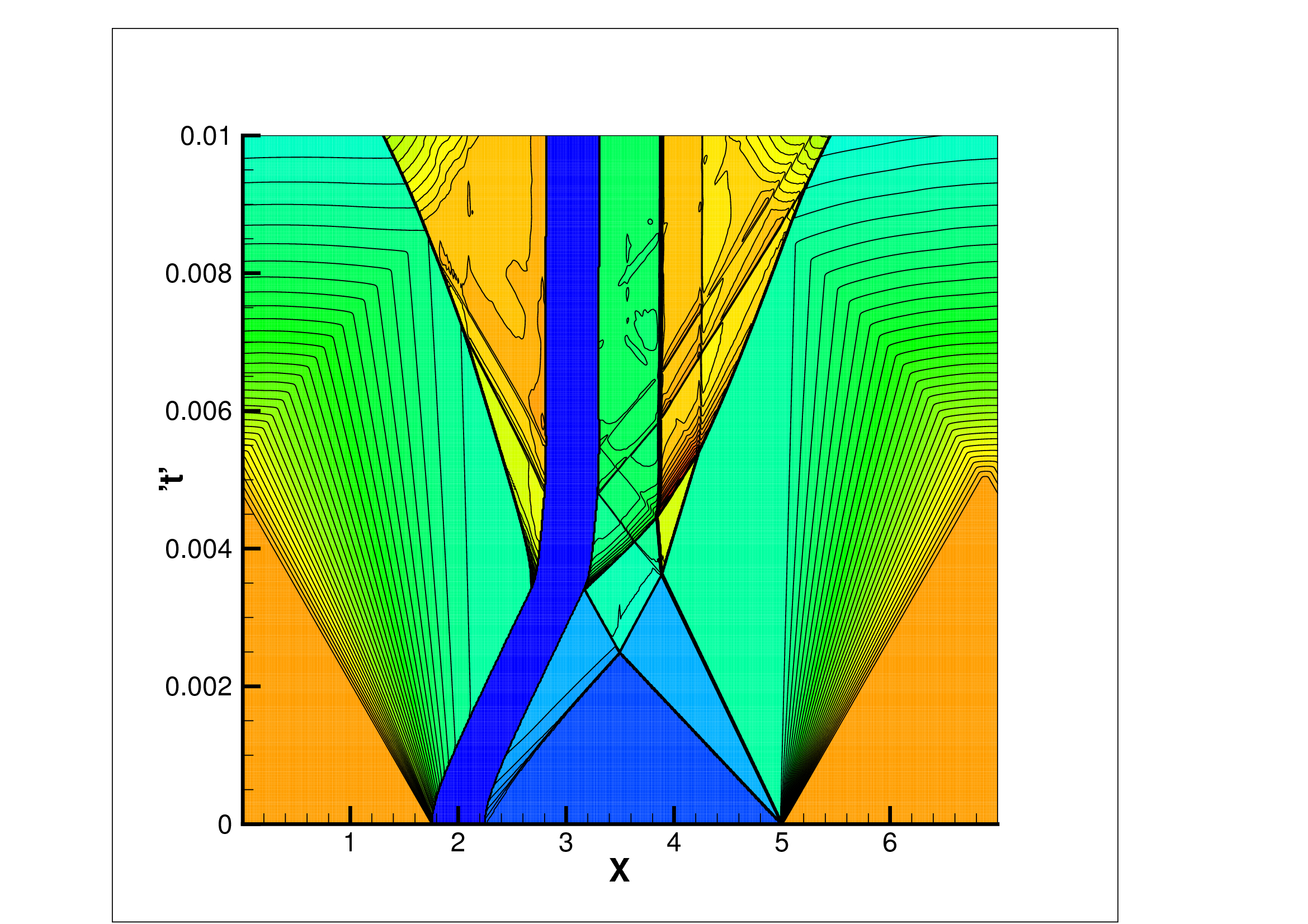
Figure 6: $x-t$ diagram (the position of the solid is in deep blue)

An ALE computation was done for comparison, using a uniform grid moving at the solid velocity. The solid position and velocity are updated using the same second-order Verlet scheme. We compared the numerical results obtained through the Embedded Boundary method on 100, 200, 400, 800, 1600, 3200, 6400 and 12800 points grids with a 51200-points ALE grid, considered as the reference solution. We observe a second-order convergence of the solid position (Figure 7) and a super-linear convergence of order 1.2 of the fluid pressure (Figure 8). The convergence rate is optimal for the solid (Verlet scheme is second-order accurate). The convergence rate for the fluid pressure is not optimal, due to the presence of discontinuities, but is not affected by the solid coupling.

Figure 7: Convergence of the solid position $L^{\infty}$-error

Figure 8: Convergence of the fluid pressure $L^{1}$-error

7.2 Double Mach reflection

A Mach 10 planar shock wave reflects on a fixed $30^{\circ}$ wedge, creating a Mach front, a reflected shock wave, and a contact discontinuity which develops into a jet along the solid boundary. This benchmark was first simulated on a Cartesian grid aligned with the solid boundary, using different finite volume methods [27, 48, 8]. Non-aligned grid methods were also tested on this benchmark, using Embedded Boundary methods [43, 7], non-conservative Immersed Boundary methods [21], $h$-box methods [24], and kinetic schemes [31]. The position of the tip of the jet is an important characteristic of the accuracy of the results. The comparison with grid-aligned results shows that it is better recovered by conservative methods than non-conservative methods [43, 7].

We have simulated the problem on a grid aligned with the wedge (aligned case, Figure 9) and on a grid aligned with the incident shock wave (non-aligned case, Figure 10). The two results are very similar, and agree with [7, 43, 27, 8]. One can remark that all the features of the flow are captured at the correct position in the non-aligned case. The jet propagates along the wall without numerical friction due to the conservation of free slip along a straight boundary (section 6.2). In the principal Mach stem, the discontinuities are slightly more oscillatory than in the aligned case. This can be identified as a post-shock oscillation phenomenon to which Roe’s scheme is especially prone (see, for instance, [28, 4]), and is not related to the coupling method. Nevertheless, the perturbations stay localized in the vicinity of discontinuities.

Figure 9: Aligned case: 30 contours of fluid density from 1.73 to 21, $\varDelta x=\varDelta y=1/220$

Figure 10: Non-aligned grid case: 30 contours of fluid density from 1.73 to 21, $\varDelta x=\varDelta y=1/220$

7.3 Lift-off of a cylinder

This moving body test case was first proposed in [14], using a conservative method. A rigid cylinder of density $7.6\text{kg.m}^{-3}$ and diameter $0.1\text{ m}$, initially resting on the lower wall of a $1\text{m}\times 0.2\text{m}$ two-dimensional channel filled with air at standard conditions ($\rho=1\text{ kg.m}^{-3}$, $p=1\text{ Pa}$), is driven and lifted upwards by a Mach 3 shock wave. Gravity is not taken into account. The problem was simulated in [20, 3, 25, 46]. In Figure 11, we present our results on a uniform $1600\times 320$ grid at times $0.14\text{ s}$ and $0.255\text{ s}$. The cylinder was approximated by a polygon with 1240 faces.

Our results agree well on the position of the solid and of the shocks with Arienti et al. [3] and Hu et al. [25]. However, some differences should be noted. First of all, some reflected shock waves in our results seem to lag slightly behind their position in previous results. This difference might be caused by small differences in the final position of the solid. Hu et al. [25] also discuss the presence of a strong vortex under the cylinder in the results of Forrer and Berger [20]. They dismiss it as an effect of the space-time splitting scheme employed which affects the numerical dissipation. We also obtain this vortex, which does not disappear as we refine the mesh. We rather believe that this vortex is associated with a Kelvin-Helmholtz instability of the contact discontinuity present under the cylinder (Figure 12).

In Figures 13 and 14 we present convergence results on the final position of the center of mass of the cylinder, compared to those of Hu et al. [25]. We observe that our results exhibit a fast convergence process, which is not the case in [25]. Let us note that no exact solution exists for the final position of the cylinder. The final position we found is however in the same range as in [25]. The results also compare well with Arienti et al. [3]. The improvement lies in the combination of the conservative interface method [25] with a conservative coupling and a second-order time-scheme for the rigid body motion. For this difficult case, the maximal conservation relative errors due to coupling were bounded by $4.10^{-6}$ over the whole simulation time, and no drift was observed.

In Figure 15 we present the relative computational cost of the coupling. The relative cost is defined as the ratio of the computational times dedicated to the coupling method and to the fluid and solid methods. In the rigid body case, the cost of the solid method is very low compared to that of the fluid method. As the coupling method is explicit and local, the computational cost is located on a manifold one dimension lower than the dimension of the whole space. In the two-dimensional case, the coupling is on a one-dimensional manifold. Indeed, we observe in Figure 15 that the relative cost of the coupling decreases as the grid is refined, with a slope of $0.5$, and that the coupling cost remains lower than the fluid and solid costs, amounting to approximately 10–20% for the grids yielding sufficient accuracy.

Figure 11: 60 contours of fluid pressure from 0 to 28 at different times, $\varDelta x=\varDelta y=6.25\times 10^{-4}$

Figure 12: 60 contours of fluid density from 0 to 12 at final time, $\varDelta x=\varDelta y=6.25\times 10^{-4}$

Figure 13: Comparison of the convergence of the horizontal position of the center of mass of the cylinder with Hu et al. [25]

Figure 14: Comparison of the convergence of the vertical position of the center of mass of the cylinder with Hu et al. [25]

Figure 15: Ratio between the coupling computation cost and the fluid and solid costs

7.4 Flapping doors

We propose this new fluid-structure interaction case as a demonstration of the robustness of our approach and as a first step towards fracture and impact simulations. The flapping doors case involves separating or closing solid boundaries, with cells including several moving boundaries. The algorithm is shown to be able to deal with such difficulties. Two doors initially close a canal and are impacted from the left by a Mach 3 shock. The canal consists of two fixed rigid walls, 2m long and 0.5m apart. Each door consists of a 0.2-m long and 0.05m-wide rectangle, completed at both ends by a half-circle of diameter 0.05m. The doors are respectively fixed on points $(0.5,0.025)$ and $(0.5,0.475)$ at the center of the half-circles. They can rotate freely around these points. The Mach 3 shock is initially located at $x=0.43$m. The density of the solid is $0.1$ kg.m^-3 and the pre- and post-shock state of the fluid are $(\rho,u,v,p)=(1,0,0,1)$ and $(\rho,u,v,p)=(3.857,2.6929,0,10.333)$. In Figure 16 we show the density field obtained using a 1600x400 grid, at times $0.125$s, $0.25$s, $0.375$s and $0.5$s. After the incident shock hits the doors, it reflects to the left and the doors open due to the high rise in pressure. The opening of the doors produces a jet preceded by a shock wave propagating to the right. Then complex interactions of waves occur, due to door movements and interaction with the walls. Kelvin-Helmholtz instabilities of contact lines can be observed at t=0.5s. It is worth noting that symmetry of the flow about the centerline of the canal axis is remarkably well preserved by the coupling method.

As the doors remain tangent to the canal walls during their rotation, the fluid cannot pass between the wall and a door at its hinge. When the doors approach the walls at maximum rotation, the fluid is compressed, and eventually pushes them back. This is observed at time $t=0.2162$s and $t=0.486$s in Figure 17, which presents the time evolution of the doors rotation angle. In the first case, the distance between each door’s straight boundary and the wall is less than 0.002m, while the size of a fluid cell is $\Delta x=0.00125$m. The method is able to deal with the fact that most cells along the wall are cut by the moving boundary and contain several moving boundaries. Treating this test case with an ALE method would require several remeshings in the course of the simulation, especially in the initial separation of the tangent door tips, and when the doors approach the walls.

Figure 16: Density contours at times $t=0.125$s (a), $t=0.25$s (b), $t=0.375$s (c) and $t=0.5$s (d)

Figure 17: Time evolution of the rotation of a door

8 Conclusion

We have presented a new coupling algorithm between a compressible fluid flows and a rigid body using an Embedded Boundary method. This explicit algorithm has the advantage of preserving the usual CFL stability condition: the time-step can be taken as the minimum of the full cell size fluid and solid time-steps. The combination of the Embedded Boundary method for the fictitious fluid domain and of the coupling strategy ensures the conservation of fluid mass and the balance of momentum and energy between fluid and solid. In addition, the exact conservation of the two constant states described in section 6 gives good insight on the consistency of the method: we prove the conservation of a constant flow in which a solid moves at the same velocity and the fact that the treatment at the boundary introduces no spurious roughness or boundary layers. The numerical examples suggest the second-order convergence of the solid position and the super-linear convergence of the fluid state in $L^{1}$ norm, while our results on two-dimensional benchmarks agree very well with body-fitted methods and improve Immersed Boundary results. We are also capable of dealing with solid boundaries moving close to each other, which is promising for impact simulations. The method is computationally efficient, as the coupling adds an integration on a space one dimension smaller than the fluid and solid computation spaces. The present method is therefore perfectly liable to be extended to a deformable solid, and was designed to extend naturally in three space dimensions. The remaining difficulty is the ability to define and track the solid boundary surrounding a Discrete Element assembly.

References

• [1] R. Abgrall. How to prevent pressure oscillations in multicomponent flow calculations: A quasi conservative approach. J. Comput. Phys., 125:150–160, 1996.
• [2] N. Aquelet, M. Souli, and L. Olovsson. Euler-lagrange coupling with damping effects : Application to slamming problems. Comput. Methods Appl. Mech. Engrg., 195(1-3):110–132, 2006.
• [3] R. Arienti, P. Hung, E. Morano, and J.E. Shepherd. A level set approach to Eulerian-Lagrangian coupling. J. Comput. Phys., 185:213–251, 2003.
• [4] M. Arora and P.L. Roe. On postshock oscillations due to shock capturing schemes in unsteady flows. J. Comput. Phys., 130:25–40, 1997.
• [5] O. Boiron, G. Chiavassa, and R. Donat. A high-resolution penalization method for large mach number flows in the presence of obstacles. J. Comp. Fluid, 38(3):703–714, 2009.
• [6] J.-I. Choi, R. C. Oberoi, J. R. Edwards, and J. A. Rosati. An immersed boundary method for complex incompressible flows. J. Comput. Phys., 224(2):757–784, 2007.
• [7] P. Colella, D.T. Graves, B.J. Keen, and D. Modiano. A Cartesian grid embedded boundary method for hyperbolic conservation laws. J. Comput. Phys., 211:347–366, 2006.
• [8] V. Daru and C. Tenaud. High order one-step monotonicity-preserving schemes for unsteady compressible flow calculations. J. Comput. Phys., 193(2):563–594, 2004.
• [9] V. Daru and C. Tenaud. Numerical simulation of the viscous shock tube problem by using a high resolution monotonicity-preserving scheme. Comput. Fluids, 38(3):664–676, 2009.
• [10] M. de Tullio and G. Iaccarino. Immersed boundary technique for compressible flow simulations on semi-structured meshes. CTR Annual Research Briefs, Center for Turbulence Research, NASA Ames/Stanford Univ., 2005.
• [11] J. Donea, S. Giuliani, and J.P. Halleux. An arbitrary Lagragian Eulerian finite element method for transient dynamic fluid-structure interactions. Comput. Methods Appl. Mech. Engrg, 33:689–723, 1982.
• [12] Z. Dragojlovic, F. Najmabadi, and M. Day. An embedded boundary method for viscous, conducting compressible flow. J. Comput. Phys., 216(1):37–51, 2006.
• [13] E. A. Fadlun, R. Verzicco, P. Orlandi, and J. Mohd-Yusof. Combined immmersed-boundary finite-difference methods for three-dimensional complex flow simulations. J. Comput. Phys., 161(1):35–60, 2000.
• [14] J. Falcovitz, G. Alfandary, and G. Hanoch. A two-dimensional conservation laws scheme for compressible flows with moving boundaries. J. Comput. Phys., 138:83–102, 1997.
• [15] C. Farhat, K.G. van der Zee, and P. Geuzaine. Provably second-order time-accurate loosely-coupled solution algorithms for transient nonlinear computational aeroelasticity. Comput. Methods Appl. Mech. Engrg., 195:1973–2001, 2006.
• [16] N. Favrie, S.L. Gavrilyuk, and R. Saurel. Solid-fluid diffuse interface model in cases of extreme deformation. J. Comput. Phys., 228:6037–6077, 2009.
• [17] R.P. Fedkiw. Coupling an Eulerian fluid calculation to a Lagrangian solid calculation with the Ghost Fluid method. J. Comput. Phys., 175:200–224, 2002.
• [18] R.P. Fedkiw, T. Aslam, B. Merriman, and S. Osher. A non-oscillatory Eulerian approach to interfaces in multimaterial flows (the Ghost Fluid method). J. Comput. Phys., 152:457–492, 1999.
• [19] M.A. Fernández, J.-F. Gerbeau, and C. Grandmont. A projection semi-implicit scheme for the coupling of an elastic structure with an incompressible fluid. Int. J. Numer. Meth. Engrg., 69:794–821, 2007.
• [20] H. Forrer and M. Berger. Flow simulation on Cartesian grids involving complex moving geometries flows, volume 129 of Int. Ser. Numer. Math. Birkhäuser, 1998.
• [21] H. Forrer and R. Jeltsch. A high-order boundary treatment for Cartesian-grid methods. J. Comput. Phys., 140:259–277, 1998.
• [22] J. Glimm, X. Li, Y. Liu, Z. Xu, and N. Zhao. Conservative front tracking with improved accuracy. SIAM J. Numer. Anal., 39:179–200, 2003.
• [23] E. Hairer, C. Lubich, and G. Wanner. Geometric Numerical Integration : Structure-Preserving Algorithms for Ordinary Differential Equations, volume 31 of Springer Series in Comput. Mathematics. Springer-Verlag, 2nd edition, 2006.
• [24] C. Helzel, M.J. Berger, and R.J. Leveque. A high-resolution rotated grid method for conservation laws with embedded geometries. SIAM J. Sci. Comput., 26:785–809, 2005.
• [25] X. Y. Hu, B. C. Khoo, N. A. Adams, and F. L. Huang. A conservative interface method for compressible flows. J. Comput. Phys., 219(2):553–578, 2006.
• [26] S. R. Idelsohn, J. Marti, A. Limache, and E. Onate. Unified Lagrangian formulation for elastic solids and incompressible fluids: Application to fluid-structure interaction problems via the PFEM. Comput. Meth. Appl. Mech. Eng., 197(19–20):1762–1776, 2008.
• [27] G-S. Jiang and C-W. Shu. Efficient implementation of Weighted ENO schemes. J. Comput. Phys., 126:202–228, 1996.
• [28] Shi Jin and Jian-Guo Liu. The effects of numerical viscosities : I. Slowly moving shocks. J. Comput. Phys., 126:373–389, 1996.
• [29] G. Kalitzin and G. Iaccarino. Turbulence modeling in an immersed-boundary rans method. CTR Annual Research Briefs, Center for Turbulence Research, NASA Ames/Stanford Univ., 2002.
• [30] G. Kalitzin and G. Iaccarino. Towards immersed boundary simulation of high reynolds number flows. CTR Annual Research Briefs, Center for Turbulence Research, NASA Ames/Stanford Univ., 2003.
• [31] B. Keen and S. Karni. A second order kinetic scheme for gas dynamics on arbitrary grids. J. Comput. Phys., 205:108–130, 2005.
• [32] Michel Lesoinne and Charbel Farhat. Geometric conservation laws for flow problems with moving boundaries and deformable meshes, and their impact on aeroelastic computations. Comput. Methods Appl. Mech. Engrg., 134:71–90, 1996.
• [33] R. J. Leveque and Z. Li. The immersed interface method for elliptic equations with discontinuous coefficients and singular sources. SIAM J. Numer. Anal., 31(4):1019–1044, 1994.
• [34] R. J. LeVeque and Z. Li. Immersed interface methods for stokes flow with elastic boundaries or surface tension. SIAM J. Sci. Comput., 18(3):709–735, 1997.
• [35] C. Mariotti. Lamb’s problem with the lattice model Mka3D. Geophys. J. Int., 171:857–864, 2007.
• [36] G. H. Miller and P. Colella. A conservative three-dimensional Eulerian method for coupled solid-fluid shock capturing. J. Comput. Phys., 183(1):26–82, 2002.
• [37] J. Mohd-Yusof. Combined immersed-boundary/b-spline methods for simulation of flow in complex geometries. CTR Annual Research Briefs, Center for Turbulence Research, NASA Ames/Stanford Univ., 1997.
• [38] L. Monasse and C. Mariotti. An energy-preserving Discrete Element Method for elastodynamics. submitted.
• [39] W.F. Noh. Fundamental methods of hydrodynamics, volume 3 of Methods of computational physics, pages 117–179. Academic Press, New York/London, 1964.
• [40] L. Olovsson. On the arbitrary Lagragian-Eulerian Finite Element Method. PhD thesis, Linköping University, 2000.
• [41] A. Paccou, G. Chiavassa, J. Liandrat, and K. Schneider. A penalization method applied to the wave equation. C. R. Mécanique, 333(1):79–85, 2005.
• [42] P. De Palma, M. D. de Tullio, G. Pascazio, and M. Napolitano. An immersed-boundary method for compressible viscous flows. Comp. Fluid, 35(7):693–702, 2006.
• [43] R.B. Pember, J.B. Bell, P. Colella, W.Y. Crutchfield, and M.L. Welcome. An adaptive Cartesian grid method for unsteady compressible flow in irregular regions. J. Comput. Phys., 120:278–304, 1995.
• [44] C. S. Peskin. Flow patterns around heart valves : A digital computer method for solving the equations of motion. PhD thesis, Albert Einstein College of Medicine, 1972.
• [45] C.S. Peskin. The immersed boundary method. Acta Numer., 11:1–39, 2002.
• [46] S.K. Sambasivan and H.S. UdayKumar. Ghost Fluid method for strong shock interactions Part 2 : Immersed solid boundaries. AIAA J., 47(12):2923–2937, 2009.
• [47] G. Strang. On construction and comparison of difference schemes. SIAM J. Numer. Anal., 5:506–516, 1968.
• [48] P. Woodward and P. Colella. The numerical simulation of two-dimensional fluid flow with strong shocks. J. Comput. Phys., 54:115–173, 1984.
• [49] S. Xu and Z. Jane Wang. An immersed interface method for simulating the interaction of a fluid with moving boundaries. J. Comput. Phys., 216(2):454–493, 2006.