Magnetic properties and thermal entanglement on a triangulated Kagomé lattice

Abstract

The magnetic and entanglement thermal (equilibrium) properties in spin-$1/2$ Ising-Heisenberg model on a triangulated Kagomé lattice are analyzed by means of variational mean-field like treatment based on Gibbs-Bogoliubov inequality. Because of the separable character of Ising-type exchange interactions between the Heisenberg trimers the calculation of quantum entanglement in a self-consistent field can be performed for each of the trimers individually. The concurrence in terms of three qubit isotropic Heisenberg model in effective Ising field is non-zero even in the absence of a magnetic field. The magnetic and entanglement properties exhibit common (plateau and peak) features observable via (antferromagnetic) coupling constant and external magnetic field. The critical temperature for the phase transition and threshold temperature for concurrence coincide in the case of antiferromagnetic coupling between qubits. The existence of entangled and disentangled phases in saturated and frustrated phases is established.

1 Introduction

Geometrically frustrated spin systems exhibit a fascinating new phases of matter, a rich variety of unusual ground states and thermal properties as a result of zero and finite temperature phase transitions driven by quantum and thermal fluctuations respectively [2, 3, 4, 1, 5, 6]. The quantum statistical studies of perplexing physics due to quantum fluctuations, geometric frustration, competing phases and complex connectivity in electron and spin lattices still remain a challenging theoretical problem. Some prominent properties related to the frustrated models, such as transition from disordered quantum spin liquid into spin insulator with broken translational symmetry similar to the Mott-Hubbard insulator at half filling with antiferromagnetic plateau behavior, seen in magnetization versus magnetic field at low-temperature, have been recently intensively studied both experimentally [7, 8, 10, 9] and theoretically [11, 13, 12]. Furthermore, the (non-bipartite) frustrated local geometry in two and three dimensions can provide also insight into the magnetism of strongly correlated electrons in small and large bipartite and non-bipartite (frustrated) Hubbard lattices also away from half filling [14]. The efforts aimed at better understanding of the aforementioned phenomena stimulated an intensive search of two-dimensional geometrically frustrated topologies, such as recently fabricated metalo-organic compound piperazinium hexachlorodicuprate [15], $\mathrm{AgNiO_{2}}$ triangular magnet [16], crystal samples of $\mathrm{KFe_{3}(OH)_{6}(SO_{4})_{2}}$ (as an ideal Kagomé lattice antiferromagnet) [17], alternating Kagomé and triangular planar layers stacked along the $[111]$ direction of the pyrochlore lattice [18], etc. Besides, studies of inorganic molecular materials with paramagnetic metal centers connected in the crystal lattice via superexchange pathways, strongly frustrated by their geometric arrangement, has also been implemented [19]. From this perspective, the most interesting geometrically frustrated topologies are the magnetic materials in form of two-dimensional isostructural polymeric coordination compounds $\mathrm{Cu_{9}X_{2}(cpa)_{6}\cdot nH_{2}O}$ ($\mathrm{X=F}$, $\mathrm{Cl}$, $\mathrm{Br}$ and cpa=carboxypentonic acid) [21, 22, 20]. The magnetic lattice of these series of compounds consists of copper ions placed at two non-equivalent positions, which are shown schematically as open and full circles in figure 2.1. $\mathrm{Cu^{2+}}$ ions with a square pyramidal coordination (a-sites) form equilateral triangles (trimers) which are connected one to another by $\mathrm{Cu^{2+}}$ ions (monomers) with an elongated octahedron environment (b-sites) forming the sites of Kagomé lattice. This magnetic architecture, which can be regarded as triangulated (triangles in triangles) Kagomé lattice, is currently under active theoretical investigation [23, 24].

The spin-$\frac{1}{2}$ Ising model on the triangulated Kagomé lattice has been exactly solved in [25]. However, in its initial form theory fails to describe the properties of the aforementioned compound series, since it entirely neglects quantum fluctuations firmly associated with a quantum nature of the paramagnetic $\mathrm{Cu^{2+}}$ ions having the lowest possible quantum spin number 1/2. Further extension to the Ising-Heisenberg model by accounting for quantum interactions between $\mathrm{Cu^{2+}}$ ions in $a$-sites (with quantum spin number 1/2) in the limit when monomeric $b$-spins having an exchange of Ising character, provides much more richer physics and displays essential features of the copper based coordination compounds [26, 27]. The strong antiferromagnetic coupling has been assumed for $J_{aa}$ between trimeric $a$ sites, while there exists a weaker ferromagnetic exchange $J_{ab}$ between the trimer $a$- and monomer $b$-sites at the ratio $|J_{ab}/J_{aa}|\approx 0,025$ [28].

Entanglement is a generic feature of quantum correlations in systems, which cannot be quantified classically [29, 30]. It provides a new perspective to understand the quantum phase transitions (QPTs) and collective phenomena in many-body and condensed matter physics. This problem, which has been under scrutiny for nearly two decades, has attracted much attention recently [31, 32, 33, 34].

A key observation is that quantum entanglement can play an important role in proximity to the QPTs, controlled by quantum fluctuations near quantum critical points [35]. A new line research points to a connection between the entanglement of a many-particle system and the existence of the QPTs and scaling [36, 37, 38]. Thermal entanglement was detected by experimental observations in low dimensional spin systems formed in the compounds Na₂Cu₅Si₄O₁₄ [39], CaMn₂Sb₂ [40], pyroborate MgMnB₂O₅ the warwickite MgTiOBO₃ [41], KNaMSi₄O₁₀ (M=Mn, Fe or Cu) [42] and metal carboxylates from magnetic susceptibility measurements [43]. Entanglement properties for few spins or electrons can display the local intrinsic features of large thermodynamic systems and can be suitable for calculations of basic magnetic quantities and various measures in entanglement associated with QPTs. The basic features of entanglement in spin-$\frac{1}{2}$ finite systems are fairly well understood by now (see e.g. [44, 45]), while the role of local cluster topology and spin correlations in thermodynamic limit still remain unanswered. There are some approximate methods, such as mean-field like theories based on the Gibbs-Bogoliubov inequality, that one can invoke to deal with the cases like this, aimed at better understanding of different physical aspects [46]. This method can also be applied for studying thermal entanglement of many-body systems [47]. In spite of the method not being exact, it is still possible to observe regions of criticality [48].

In the case of the triangulated Kagomé lattice each $a$-type trimer interacts with its neighboring trimer through the Ising-type exchange, i.e. classical interaction, therefore the states of two neighboring $a$-sublattices become separable (disentangled) [29]. Thus we can calculate concurrence (a measure of entanglement [49]), which characterizes quantum features, for each trimer separately in self-consistent field. The key result of the paper is concentrated on the comparison of specific (peak and plateau) features in magnetization, susceptibility, specific heat and thermal entanglement properties in the above mentioned model using variational mean-field like approximation based on Gibbs-Bogoliubov inequality. We will demonstrate how the order-disorder phase transition temperature is relevant to the the threshold temperature for vanishing of entanglement.

The rest of the paper is organized as follows: in section 2 we introduce the Ising-Heisenberg model on the triangulated Kagomé lattice and provide a solution in variational mean-field like approximation based on Gibbs-Bogoliubov inequality. The magnetic properties of the model are investigated in section 3. The basic principles for calculation of concurrence as a measure of entanglement and some of the results on intrinsic properties are introduced in section 4. In section 5 we present the comparison of magnetic properties and thermal entanglement. The concluding remarks are given in section 6.

2 Isotropic Heisenberg model on triangulated Kagomé lattice

2.1 Spin-$\frac{1}{2}$ Ising-Heisenberg model

We consider the spin-$\frac{1}{2}$ Ising-Heisenberg model on triangulated Kagomé lattice (TKL) (figure 2.1) consisting of two types of sites ($a$ and $b$). Since the exchange coupling between $\mathrm{Cu}^{2+}$ ions are almost isotropic, the application of the $XXX$ Heisenberg model is more appropriate. There is a strong Heisenberg $J_{aa}$ exchange coupling between trimeric sites of $a$ type and weaker Ising-type one ($J_{ab}$) between trimeric $a$ and monomeric $b$ ones. Thus, the Kagomé lattice of the Ising spins (monomers) contains inside of each triangle unit a smaller triangle of the Heisenberg spins (trimer). The Hamiltonian can be written as follows:

$${\mathcal{H}}=J_{aa}\sum_{(i,j)}\mathbf{S}^{a}_{i}\mathbf{S}^{a}_{j}-J_{ab}\sum_{(k,l)}(S^{z})^{a}_{k}\cdot(S^{z})^{b}_{l}-H\sum_{i=1}^{\frac{2N}{3}}3[(S^{z})^{a}_{j}+\frac{1}{2}(S^{z})^{b}_{j}],$$ (1)

where $\mathbf{S}^{a}=\{S^{a}_{x},S^{a}_{y},S^{a}_{z}\}$ is the Heisenberg spin-$\frac{1}{2}$ operator, $S^{b}$ is the Ising spin. $J_{aa}>0$ corresponds to antiferromagnetic Heisenberg coupling and $J_{ab}>0$ to ferromagnetic Ising-Heisenberg one. The first two summations run over $a-a$ and $a-b$ nearest neighbors respectively and the last sum incorporates the effect of uniform magnetic field (we have assumed that the total number of sites is $3N$).

Figure 1: A cross-section of TKL structure. Solid lines represent the intra-trimer Heisenberg interactions $J_{aa}$, while the broken ones label monomer-trimer Ising interactions $J_{ab}$. The circle marks $k$-th cluster (Heisenberg trimer). $\mathbf{S}^{a}_{k_{i}}$ presents the Heisenberg and $S^{b}_{k_{i}}$ the Ising spins.

2.2 Basic mean-field formalism

Here we apply the variational mean-field like treatment based on Gibbs-Bogoliubov inequality [50] to solve the Hamiltonian (1). This implies that the free energy (Helmholtz potential) of system is

$$F\leq F_{0}+\langle{\mathcal{H}}-{\mathcal{H}_{0}}\rangle_{0},$$ (2)

where $\mathcal{H}$ is the real Hamiltonian which describes the system and $\mathcal{H}_{0}$ is the trial one. $F$ and $F_{0}$ are free energies corresponding to $\mathcal{H}$ and $\mathcal{H}_{0}$ respectively and $\langle...\rangle_{0}$ denotes the thermal average over the ensemble defined by $\mathcal{H}_{0}$. Following [23] we introduce the trial Hamiltonian in the following form:

$$\mathcal{H}_{0}= \sum_{k\in trimers}\mathcal{H}_{c_{0}},$$ (3a)

$$\mathcal{H}_{c_{0}}= \lambda_{aa}\left(\mathbf{S}^{a}_{k_{1}}\mathbf{S}^{a}_{k_{2}}+\mathbf{S}^{a}_{k_{2}}\mathbf{S}^{a}_{k_{3}}+\mathbf{S}^{a}_{k_{1}}\mathbf{S}^{a}_{k_{3}}\right)-\sum_{i=1}^{3}\left[\gamma_{a}(S^{z})^{a}_{k_{i}}+\frac{\gamma_{b}}{2}(S^{z})^{b}_{k_{i}}\right].$$ (3b)

In this Hamiltonian the stronger quantum Heisenberg antiferromagnetic interactions between $a$-sites are treated exactly, while the weaker Ising-type ones between $a$- and $b$-sites are replaced by self-consistent (effective) fields of two types: $\gamma_{a}$ and $\gamma_{b}$. The variational parameters $\gamma_{a}$, $\gamma_{b}$ and $\lambda_{aa}$ can be found from the Bogoliubov inequality after minimizing the RHS of (2). Thus our focus is on the cluster depicted in figure 2.1. Each of the $b$-type spins belongs to two of such clusters simultaneously. Hence only the half of each $b$-spin belongs to one cluster and therefore there are $3\cdot 1/2$ b-type spins in it. Consequently the total number of ($a-$ and $b-$) spins in the cluster will be $3+3/2=9/2$ (there are $3$ $a$-type spins in the triangle). Inequality (2) can be rewritten for the described cluster:

$$f\leq f_{0}+\langle{\mathcal{H}_{c}}-\mathcal{H}_{c_{0}}\rangle_{0},$$ (3d)

where $\mathcal{H}_{c}$ is the real and $\mathcal{H}_{c_{0}}$ the trial Hamiltonian of the cluster, $f$ and $f_{0}$ free energies of the cluster defined by $\mathcal{H}_{c}$ and $\mathcal{H}_{c_{0}}$ respectively. Using the fact that in terms of (3b) $\mathbf{S}^{a}$ and $\mathbf{S}^{b}$ are statistically independent, one obtains $\langle\mathbf{S}^{a}\cdot\mathbf{S}^{b}\rangle_{0}=\langle\mathbf{S}^{a}\rangle_{0}\cdot\langle\mathbf{S}^{b}\rangle_{0}$. Besides, taking into account that $\langle{(S^{z})^{a}}\rangle_{0}=m_{a}$ (single $a$-site magnetization), $\langle{(S^{z})^{b}}\rangle_{0}=m_{b}$ (single $b$-site magnetization), we obtain the following expression:

$$f\leq f_{0}+(J_{aa}-\lambda_{aa})\langle\mathbf{S}^{a}_{k_{1}}\mathbf{S}^{a}_{k_{2}}+\mathbf{S}^{a}_{k_{2}}\mathbf{S}^{a}_{k_{3}}+\mathbf{S}^{a}_{k_{1}}\mathbf{S}^{a}_{k_{3}}\rangle_{0}$$ (3e)

$$-6J_{ab}m_{a}m_{b}-3Hm_{a}-\frac{3Hm_{b}}{2}+3\gamma_{a}m_{a}+\frac{3\gamma_{b}m_{b}}{2}.$$

Now, by minimizing the right-hand side of inequality (3e) with respect to $\gamma_{a}$, $\gamma_{b}$ and $\lambda_{aa}$ and using $\frac{\partial f_{0}}{\partial\gamma_{a}}=-3m_{a}$, $\frac{\partial f_{0}}{\partial\gamma_{b}}=-3/2m_{b}$, $\frac{\partial f_{0}}{\partial\lambda_{aa}}=\langle\mathbf{S}^{a}_{k_{1}}\mathbf{S}^{a}_{k_{2}}+\mathbf{S}^{a}_{k_{2}}\mathbf{S}^{a}_{k_{3}}+\mathbf{S}^{a}_{k_{1}}\mathbf{S}^{a}_{k_{3}}\rangle_{0}$, we determine the variational parameters in the form: $\lambda_{aa}=J_{aa}$, $\gamma_{a}=2J_{ab}m_{b}+H$, $\gamma_{b}=4J_{ab}m_{a}+H$. Parameters $\gamma_{a}$ and $\gamma_{b}$, which have a meaning of a magnetic field, are interconnected, which is the consequence of its‘ apparent self-consistency. The Hamiltonian $\mathcal{H}_{0}$ was chosen to be exactly solved. One finds that $\mathcal{H}_{c_{0}}$ can be divided into two parts corresponding to $a$- and $b$-type variables:

$$\mathcal{H}_{c_{0}}= \left[\lambda_{aa}\{\mathbf{S}^{a}_{k_{1}}\mathbf{S}^{a}_{k_{2}}+\mathbf{S}^{a}_{k_{2}}\mathbf{S}^{a}_{k_{3}}+\mathbf{S}^{a}_{k_{1}}\mathbf{S}^{a}_{k_{3}}\}-\sum_{i=1}^{3}\gamma_{a}(S^{z})^{a}_{k_{i}}\right]-\sum_{i=1}^{3}\frac{\gamma_{b}}{2}(S^{z})^{b}_{k_{i}}$$ (3f)

$$=\mathcal{H}_{c_{0}}^{a}+\sum_{i=1}^{3}(\mathcal{H}_{c_{0}}^{b})^{i}.$$

Each of Hamiltonians $\mathcal{H}_{c_{0}}^{a}$ and $(\mathcal{H}_{c_{0}}^{b})^{i}$ can be solved separately (the variables have been separated). The eigenvalues of $\mathcal{H}_{c_{0}}^{a}$ are:

$$E_{1}=\frac{3}{4}\left(\lambda_{aa}+2\gamma_{a}\right);\quad E_{2}=E_{3}=\frac{1}{4}\left(-3\lambda_{aa}+2\gamma_{a}\right);$$

$$E_{4}=\frac{1}{4}\left(3\lambda_{aa}+2\gamma_{a}\right);\quad E_{5}=E_{6}=\frac{1}{4}\left(-3\lambda_{aa}-2\gamma_{a}\right);$$ (3g)

$$E_{7}=\frac{1}{4}\left(3\lambda_{aa}-2\gamma_{a}\right);\quad E_{8}=\frac{3}{4}\left(\lambda_{aa}-2\gamma_{a}\right)$$

and the corresponding eigenvectors given by

$$|\psi_{1}\rangle=|000\rangle$$

$$|\psi_{2}\rangle=\frac{1}{\sqrt{3}}\left(q|001\rangle+q^{2}|010\rangle+|100\rangle\right)$$

$$|\psi_{3}\rangle=\frac{1}{\sqrt{3}}\left(q^{2}|001\rangle+q|010\rangle+|100\rangle\right)$$

$$|\psi_{4}\rangle=\frac{1}{\sqrt{3}}\left(|001\rangle+|010\rangle+|100\rangle\right)$$

$$|\psi_{5}\rangle=\frac{1}{\sqrt{3}}\left(q|110\rangle+q^{2}|101\rangle+|011\rangle\right)$$ (3h)

$$|\psi_{6}\rangle=\frac{1}{\sqrt{3}}\left(q^{2}|110\rangle+q|101\rangle+|011\rangle\right)$$

$$|\psi_{7}\rangle=\frac{1}{\sqrt{3}}\left(|110\rangle+|101\rangle+|011\rangle\right)$$

$$|\psi_{8}\rangle=|111\rangle,$$

where $q=e^{i2\pi/3}$ (these eigenvectors should be also the eigenstates of cyclic shift operator $P$ with eigenvalues $1$, $q$ and $q^{2}$, satisfying $q^{2}+q+1=0$).

The partition function $Z_{0_{a}}$ of the trimer in mean-field approximation is:

$$Z_{0_{a}}=\sum_{k=1}^{8}\exp(-E_{k}/T)=e^{-\frac{3{\lambda_{aa}}}{4T}} \left[\cosh\left(\frac{3\gamma_{a}}{2T}\right)+\right.$$

$$\left.2e^{\frac{3{\lambda_{aa}}}{2T}}\cosh\left(\frac{\gamma_{a}}{2T}\right)+\cosh\left(\frac{\gamma_{a}}{2T}\right)\right].$$

Consequently the free energy of $a$-triangle will be:

$$f_{0_{a}}=-T\ln Z_{0_{a}}=\frac{3{\lambda_{aa}}}{4}-T\ln \left[\cosh\left(\frac{3\gamma_{a}}{2T}\right)+2e^{\frac{3{\lambda_{aa}}}{2T}}\cosh\left(\frac{\gamma_{a}}{2T}\right)+\right.$$

$$\left.\cosh\left(\frac{\gamma_{a}}{2T}\right)\right].$$

Since the $(\mathcal{H}_{c_{0}}^{b})^{i}$ describes only half a particle (b-type spin), the Hamiltonian of one b-type spin will be $2\cdot(\mathcal{H}_{c_{0}}^{b})^{i}$. Hence, following the technique described above one finds the partition function $Z_{0_{b}}$ and free energy $f_{0_{b}}$ of a b-type spin in the adopted approximation:

$$Z_{0_{b}}=2\cosh\left(\frac{\gamma_{b}}{2T}\right),$$ (3ka)

$$f_{0_{b}}=-T\ln\left[2\cosh\left(\frac{\gamma_{b}}{2T}\right)\right].$$ (3kb)

As already mentioned, in terms of the trial Hamiltonian $a$- and $b$-type spins are statistically independent [see equations (3) and (3f)]. Besides, $b-$ type spins do not interact with each other. Therefore the partition function $f_{0}$ of the cluster in mean-field approximation reads:

$$f_{0}=f_{0_{a}}+\frac{3}{2}\cdot f_{0_{b}}.$$ (3kl)

Consequently the free energy of the cluster $f_{GB}$ in the mean-field approximation based on the Gibbs-Bogoliubov inequality will be:

$$f_{GB}= f_{0}+\langle{\mathcal{H}_{c}}-\mathcal{H}_{c_{0}}\rangle_{0}=\frac{3\lambda_{aa}}{4}+6J_{ab}m_{a}m_{b}-T\left[\ln\left\{4e^{\frac{3J_{ab}}{2T}}\cosh\left(\frac{\gamma_{a}}{2T}\right)\right.\right.$$ (3km)

$$\left.+2\cosh\left(\frac{\gamma_{a}}{2T}\right)+2\cosh\left(\frac{3\gamma_{a}}{2T}\right)\right\}\left.+\frac{3}{2}\ln\left\{2\cosh\left(\frac{\gamma_{b}}{2T}\right)\right\}\right].$$

In equation (3km) we have used the values of variational parameters $\gamma_{a}$, $\gamma_{b}$ and $\lambda_{aa}$. Besides, due to the fact that there are $9/2$ spins in the cluster and therefore totally $2N/3$ clusters ($F_{GB}=2N/3\cdot f_{GB}$), we obtain:

$$\frac{F_{GB}}{N}= \frac{\lambda_{aa}}{2}+4J_{ab}m_{a}m_{b}-2T\left[\frac{1}{3}\ln\left\{4e^{\frac{3J_{ab}}{2T}}\cosh\left(\frac{\gamma_{a}}{2T}\right)\right.\right.$$ (3kn)

$$\left.+2\cosh\left(\frac{\gamma_{a}}{2T}\right)+2\cosh\left(\frac{3\gamma_{a}}{2T}\right)\right\}\left.+\frac{1}{2}\ln\left\{2\cosh\left(\frac{\gamma_{b}}{2T}\right)\right\}\right].$$

As for defined above $a$- and $b$-single site magnetizations we obtain:

$$m_{a}= -\frac{1}{3}\frac{\partial f_{0_{a}}}{\partial\gamma_{a}}=\frac{1}{6}\frac{3\sinh\left(\frac{3\gamma_{a}}{2T}\right)+2e^{\frac{3{\lambda_{aa}}}{2T}}\sinh\left(\frac{\gamma_{a}}{2T}\right)+\sinh\left(\frac{\gamma_{a}}{2T}\right)}{\cosh\left(\frac{3\gamma_{a}}{2T}\right)+2e^{\frac{3{\lambda_{aa}}}{2T}}\cosh\left(\frac{\gamma_{a}}{2T}\right)+\cosh\left(\frac{\gamma_{a}}{2T}\right)},$$ (3koa)

$$m_{b}= -\frac{\partial f_{0_{b}}}{\partial\gamma_{b}}=\frac{1}{2}\tanh\left(\frac{\gamma_{b}}{2T}\right).$$ (3kob)

Notwithstanding of simplicity and the fact that the effective (self-consistent) field in zero magnetic field ($H=0$) overestimates ferromagnetic correlations, it is still particularly useful for detection of spontaneous breaking SU(2) symmetry and possible temperature driven transitions in the frustrated spin systems (see section 3.1). However, we also find that the strong quantum fluctuations, existing in the isotropic Heisenberg model in the absence of ferromagnetic type Ising term at $H=0$ can restore the broken symmetry by providing stability to disordered spin-$1/2$ liquid state in frustrated geometries. Moreover, in general the presence of magnetic field ($H\neq 0$) suppresses the spin fluctuations and makes the self-consistent results more reliable and accurate [51]. Therefore, the equations (7), (8) and (13)-(15) with magnetic field are quite sufficient for understanding some intrinsic relationships between magnetic and entanglement properties [44] that naturally emerge in the Ising-Heisenberg model when one is complying with the variational mean-field like procedure.

3 Magnetic properties

3.1 Magnetization

The results of the previous section can be used for investigation of the magnetic properties of the model. Here we are interested in the sublattice $a$ properties, which, however, depend on parameters describing $b$-type spins. It is convenient to introduce a new (ratio) parameter $\alpha=J_{ab}/J_{aa}$. The magnetization curves can be found by solving numerically the transcendental equations (3koa) and (3kob). The magnetic field dependence of the magnetization per atom is plotted in figure 3.1 at $\alpha=0.025$. We find that in the absence of magnetic field, the ordered ferromagnetic phase with spontaneous magnetization per site $m_{a}$ is a stable ground state for all $|J_{ab}/J_{aa}|$ in spite of the high geometric frustration caused by the non-bipartite structure and antiferromagnetic intra-trimer interaction.

(a)	(b)

Figure 2: Single $a$-site magnetization $m_{a}$ versus external magnetic field $H$ for (a) $T=0.7$ and (b) $T=0.01$ for $\alpha=0.025$, $J_{aa}=1$. The magnetic field and temperature are in relative units of $k_{B}=1$.

At relatively high temperatures the magnetization curve in figure 3.1(a) shows a monotonic behavior versus magnetic field with a full saturation at strong magnetic field. Upon decreasing the temperature a new partially saturated phase emerges in form of the (spin) plateaus shown in figure 3.1(b), which can be associated with staggered magnetization or short range antiferromagnetism (AF) in frustrated Kagomé geometry. Indeed, the appearance of plateau in magnetization curve at $m_{a}=1/6$ can be explained as stability of trimeric $a$ sites in $\uparrow\uparrow\downarrow$ configuration. Thus, at rather low temperatures, the magnetization shows the finite leap across a plateau at $m_{a}=1/6$ at infinitesimal magnetic field and below the critical field for full saturation by flipping a down spin.

In figure 3.1 we also show the temperature dependence of the magnetization in equilibrium. As one can see from figure 3.1(a), in the absence of the external magnetic field the magnetization tends gradually to zero near the second-order transition temperature $T_{c}$ between ordered ($m_{a}\neq 0$) and disordered ($m_{a}=0$) phases. Hence, the magnetization $m_{a}$ can be expanded into series near the critical temperature of second-order phase transition point:

$$m_{a}=am_{a}+bm_{a}^{3}+cm_{a}^{5}+...$$ (3kop)

The critical temperature $T_{c}$ corresponding to the second-order phase transition can be found from the condition $a=1$, $b<0$. In particular, for the case $J_{aa}=1$ and $\alpha=0.025$, $T_{c}=0.0102062$ (in relative units). At zero temperature in the absence of field we find unsaturated spontaneous ferromagnetism with $m_{a}=1/6$ as a stable ground state.

(a)	(b)

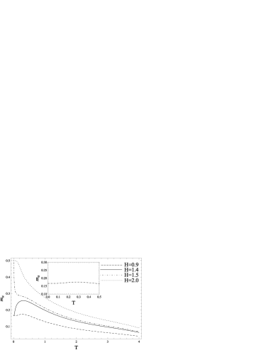
Figure 3: Single $a$-site magnetization $m_{a}$ per atom versus temperature $T$ for $J_{aa}=1$, $\alpha=0.025$ and (a) $H=0$ and (b) different non-zero values of $H$ (the inset shows details for the case $H=0.9$ at low temperatures).

The magnetization in equilibrium as a function of temperature $T$ at non-zero magnetic field [52] is plotted in figure 3.1(b). There are two distinct magnetic field regimes corresponding to $m_{a}=1/6$ and saturated zero-temperature magnetization, $m_{a}=1/2$. While fixed magnetic field $H$ is less than the saturation magnetic field value, we deal with $m_{a}=1/6$ regime. If we continue increasing the value of $H$, at the saturation magnetic field the magnetization jumps into $m_{a}=1/2$ regime [$H=1.5,$ $2.0$ in figure 3.1(b)]. There can be also seen a short plateau at $m_{a}=1/6$ in the temperature dependence [$H=0.9$ in figure 3.1(b)]. The peaks in the case of low magnetic fields arise due to the frustration effects.

3.2 Susceptibility

We define the magnetic susceptibility $\chi_{a}$ as

$$\chi_{a}=\frac{\partial m_{a}}{\partial H}.$$ (3koq)

First we examine the zero-field susceptibility, which is introduced as follows:

$$\chi_{a_{0}}=\left.\frac{\partial m_{a}}{\partial H}\right|_{H=0}.$$ (3kor)

The temperature dependence of $\chi_{a_{0}}$ in equilibrium is plotted in figure 3.2.

Figure 4: Zero-field susceptibility $\chi_{a_{0}}$ versus temperature $T$ for $J_{aa}=1$ and $\alpha=0.025$.

The zero-field susceptibility $\chi_{a_{0}}$ diverges at the critical temperature $T_{c}$ which is a signature of the second order phase transition discussed earlier (see section 3.1). The temperature dependence of susceptibility $\chi_{a}$ at $H\neq 0$ [53] is presented in figure 3.2(a).

(a)	(b)

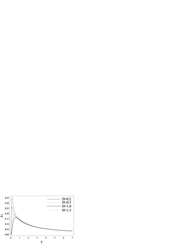
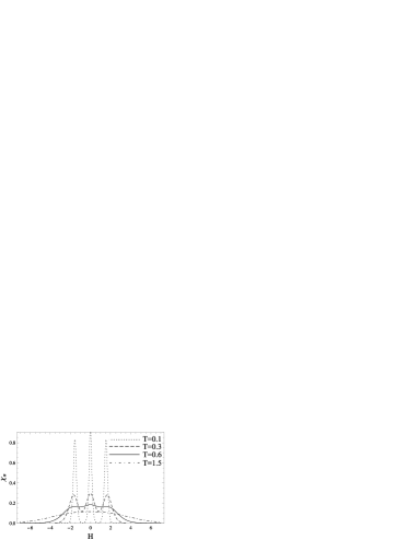
Figure 5: Susceptibility $\chi_{a}$ versus (a) temperature $T$ at different $H$ and (b) magnetic field $H$ at different $T$ for $J_{aa}=1$, $\alpha=0.025$.

The temperature dependence of magnetic susceptibility observed in [54] for $\mathrm{[Ni(H_{2}L^{2})]_{4}[Cr(CN)_{6}]_{5}OH\cdot 15H_{2}O}$ compounds resembles the result shown in figure 3.2.

Notice, that at high temperatures the external field dependence of the magnetic susceptibility [figure 3.2(b)] exhibits one peak. With decreasing temperature, two symmetric peaks begin to arise, which correspond to the formation of the incipient (magnetization) plateau at $m_{a}=1/6$. With decreasing further temperature the peaks become sharper and bigger in their magnitude.

3.3 Specific heat

The internal energy $u$ and the specific heat $c(T)$ per cluster site are, respectively, determined as

$$u=-T^{2}\frac{\partial}{\partial T}\left(F_{GB}/3NT\right)$$ (3kos)

$$c(T)=\frac{\partial u}{\partial T}=-\frac{T}{3N}\frac{\partial^{2}F_{GB}}{\partial T^{2}},$$ (3kot)

$F_{GB}$ taken from (3kn).

Figure 6: The zero-field specific $c(T)$ heat versus temperature $T$ for $J_{aa}=1$, $\alpha=0.025$.

The behavior of the specific heat in equilibrium at the absence of the external magnetic field ($H=0$) is shown in figure 3.3. In this plot one can find the presence of second order phase transition: at the same temperature $T_{c}$, described in last two subsections, the specific heat has discontinuity.

Figure 7: Specific heat $c(T)$ versus temperature $T$ for $J_{aa}=1$, $\alpha=0.025$ and different $H$ values.

The temperature dependence of the specific heat at non-zero magnetic field is shown in figure 3.3. Notwithstanding the observation of one peak in the $c(T)$ at $H=0$ the temperature dependence of specific heat at $H\neq 0$ exhibits two-peak behavior peculiar to one and quasi one dimensional systems as one can find in [55, 56]. A double-peak structure in the specific heat manifests the existence of two energy scales in the system as a result of two competing orders [57]. Upon increasing the external magnetic field the peak moves to higher-temperature region and, at the same time, decreases in amplitude. At higher values of $H$ close to the transition from $m_{a}=1/6$ to saturated $m_{a}=1/2$ state the second broad peak gradually increases.

In section 5 we further discuss magnetic properties by comparison with thermal entanglement.

4 Concurrence and thermal entanglement

The mean-field like treatment of (1) transforms many-body system to reduced ”single” cluster study in a self-consistent field where quantum interactions exist. This allows to study, in particular, (local) thermal entanglement properties of $a$-sublattice in terms of three-qubit $XXX$ Heisenberg model in effective magnetic field $\gamma_{a}$, which carries the main properties of the system. Besides, because of the self-consistency and interconnection of the fields $\gamma_{a}$ and $\gamma_{b}$ the effective $\gamma_{b}$ field have an impact on the concurrence, too. We study concurrence $C(\rho)$, to quantify pairwise entanglement [49], defined as

$$C(\rho)=max\{\lambda_{1}-\lambda_{2}-\lambda_{3}-\lambda_{4},0\},$$ (3kou)

where $\lambda_{i}$ are the square roots of the eigenvalues of the corresponding operator for the density matrix

$$\tilde{\rho}=\rho_{12}(\sigma_{1}^{y}\otimes\sigma_{2}^{y})\rho_{12}^{*}(\sigma_{1}^{y}\otimes\sigma_{2}^{y})$$ (3kov)

in descending order. Since we consider pairwise entanglement, we use reduced density matrix $\rho_{12}=\mathrm{Tr_{3}}\rho$. Before introducing the calculations and discussion we would like to emphasize the fact which was already discussed in section 1: the states of two neighboring $a$-type trimers are separable (disentangled). Hence we can calculate the concurrence for each of them on cluster level individually in effective magnetic field. In our case the density matrix has the following form

$$\rho=\frac{1}{Z_{0}{{}_{a}}}\sum_{k=1}^{8}\exp(-E_{k}/T)|\psi_{k}\rangle\langle\psi_{k}|,$$ (3kow)

$E_{k}$, $|\psi_{k}\rangle$ and $Z_{0}{{}_{a}}$ are taken from equations (7), (8) and (9) respectively. The construction process of matrix (3kov) does not depend whether $\gamma_{a}$ is effective or real magnetic field, although the presence of effective field $\gamma_{a}$ plays crucial role for the self-consistent solution. Here we skip the specific details and provide the result of final calculations of the matrix $\rho_{12}$, taking into account that the Hamiltonian $\mathcal{H}_{c_{0}}$ is translationary invariant with a symmetry $[S_{z},\mathcal{H}_{c_{0}}]=0$ ($S_{z}=\sum_{k=1}^{3}(S_{z})^{a}_{k_{i}}$). Hence [58]:

$$\rho_{12}=\left(\begin{array}[]{llll}u&0&0&0\\ 0&w&y&0\\ 0&y^{*}&w&0\\ 0&0&0&v\end{array}\right),$$ (3kox)

where

$$u=\frac{1}{3}e^{\frac{2\gamma_{a}-3\lambda_{aa}}{4T}}\left(1+3e^{\frac{\gamma_{a}}{T}}+2e^{\frac{3\lambda_{aa}}{2T}}\right)$$ (3koy)

$$v=\frac{1}{3}e^{-\frac{3\left(2\gamma_{a}+\lambda_{aa}\right)}{4T}}\left(3+e^{\frac{\gamma_{a}}{T}}+2e^{\frac{2\gamma_{a}+3\lambda_{aa}}{2T}}\right)$$ (3koz)

$$w=\frac{1}{3}e^{-\frac{2\gamma_{a}+3\lambda_{aa}}{4T}}\left(1+e^{\frac{\gamma_{a}}{T}}\right)\left(1+2e^{\frac{3\lambda_{aa}}{2T}}\right)$$ (3koaa)

$$y=-\frac{1}{3}e^{-\frac{2\gamma_{a}+3\lambda_{aa}}{4T}}\left(1+e^{\frac{\gamma_{a}}{T}}\right)\left(-1+e^{\frac{3\lambda_{aa}}{2T}}\right).$$ (3koab)

$\rho_{12}$ in equation (3kox) is a special case of so called $X$-state [59]. The concurrence $C(\rho)$ of such a density matrix has the following form [60]:

$$C(\rho)=\frac{2}{Z}max(|y|-\sqrt{uv},0).$$ (3koac)

Finally, we consider transcendental equations (3koa) and (3kob) by taking into account the values of variational parameters: $\lambda_{aa}=J_{aa}$, $\gamma_{a}=2J_{ab}m_{b}+H$, $\gamma_{b}=4J_{ab}m_{a}+H$, and, therefore, one can use these parameters to calculate $C(\rho)$. First, we study the behavior of $C(\rho)$ at $H=0$. The temperature dependence of $C(\rho)$ is shown in figure 4.

Figure 8: Concurrence $C(\rho)$ versus temperature field for $J_{aa}=1$, $\alpha=0.025$ and $H=0$

Notice, the ”triangle-in-triangle” system can display (bipartite) entanglement described by concurrence even in the absence of external magnetic field. It is important to mention that this result does not contradict to the well-known fact that there is no (bipartite) entanglement, measured by concurrence in isotropic three-qubit Heisenberg $XXX$ model in zero magnetic field ($H=0$) [44]. Indeed this effect is due to the existence of Ising-type interaction replaced by effective field $\gamma_{a}=2J_{ab}m_{b}+H$ acting upon $a$-spins. The latter, in addition to $H$ contains another quantity having meaning of magnetic ($2J_{ab}m_{b}$), which is non-zero at $H=0$.

Another important observation is that threshold temperature at which entanglement $C(\rho)$ disappear is identical to the critical temperature $T_{c}$ of second order phase transition between ordered and disordered phases described earlier in section 3.3. This implies that the concurrence vanishes precisely at $T_{c}$, the same temperature of specific heat discontinuity. This is the consequence of the fact that at $T_{c}$ the system undergoes order-disorder phase transition and the second term in $\gamma_{a}$ vanishes, too ($m_{b}=0$, when $H=0$ and $T\geq T_{c}$). This factor implies the strong relationship between magnetic and entanglement properties of the system. In figure 4 we present the three dimensional plot of the concurrence as a function of the temperature and external magnetic field. We will discuss some of these features in behavior of concurrence $C(\rho)$ for studying magnetic and entanglement thermal properties in section 5.

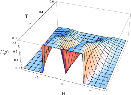
Figure 9: Concurrence $C(\rho)$ versus temperature $T$ and external magnetic field $H$ for $J_{aa}=1$, $\alpha=0.025$.

5 Common features of magnetic properties and entanglement

5.1 Finite temperatures

To the best of our knowledge, the common thermal features in entanglement and magnetic properties in frustrated systems have not yet been reported, neither theoretically, nor experimentally. In this section we discuss some similarities of magnetic statistical properties and quantum entanglement.

First, we consider for general $J_{aa}$ and $H$ the susceptibility (3koq) as a statistical characteristic. Figure 5.1 (a) shows the density distribution of susceptibility reduced per one $a$-site as a function of the coupling constant $J_{aa}$ and the external field $H$, at a relatively high temperature $T=0.1$, which is higher than $T_{c}$. The white stripes on the figure correspond to peaks of the susceptibility. These stripes have a certain finite width due to nonzero temperature. For consistency in figure 5.1 (b) a similar plot of concurrence density is shown for the same values of $J_{aa}-H$ parameters. The existence of entanglement in the infinite $XXX$ Heisenberg chains of spins-$1/2$ and spins-$1$ was pointed in [61]. Here weak probe fields have been aligned along three orthogonal directions ($x$, $y$ and $z$), supposing that magnetic susceptibility is equal in all these directions ($\chi_{x}=\chi_{y}=\chi_{z}$) and using the fact that $\chi_{x}+\chi_{y}+\chi_{z}$ is an entanglement witness. In our case there is a magnetic field aligned in the z-direction only, therefore $\chi_{z}\equiv\chi_{a}$. And we show that the behavior of susceptibility $\chi_{z}$ is similar to that of bipartite entanglement. Indeed, comparison of figures 5.1a and 5.1b shows that the general behavior of the statistical and entanglement properties, such as susceptibility ($\chi_{a}$) and concurrence ($C(\rho)$), coincide. Our calculations show that the values of variables for the maximum (peak) in magnetic susceptibility correspond to the critical values on the $J_{aa}-H$ diagram at which the quantum coherence disappear and concurrence vanishes ($C(\rho)=0$). However, this picture for the Ising-Heisenberg model on the TKL lattice can applied only for antiferromagnetic coupling $J_{aa}>0$, while for ferromagnetic coupling $J_{aa}<0$ the system always remains disentangled.

(a)	(b)

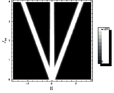
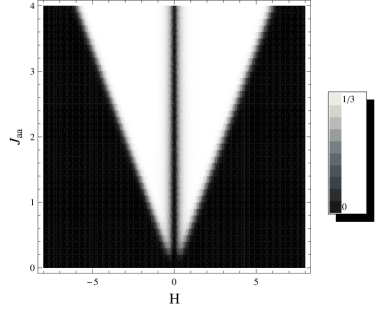
Figure 10: Density plot for (a) susceptibility $\chi_{a}$ and (b) concurrence $C(\rho)$ versus magnetic field $H$ and coupling constant $J_{aa}$ at $\alpha=0.025$ and $T=0.1$.

For further comparison we show for various temperatures in figure 5.1 (a) and (b) the corresponding dependencies of the concurrence and heat capacity on magnetic field $H$.

(a)	(b)

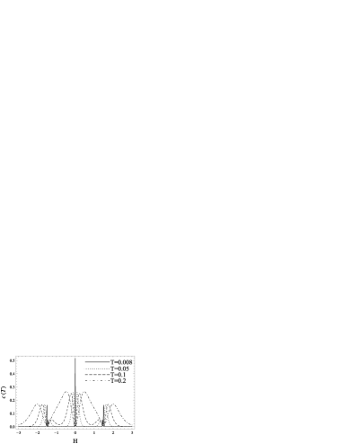
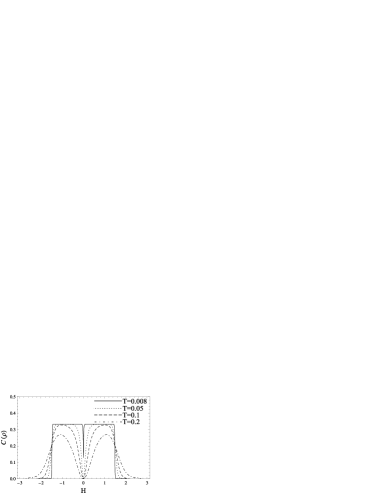
Figure 11: (a) Specific heat $c(T)$ and (b) concurrence $C(\rho)$ versus external magnetic field $H$ for $J_{aa}=1$, $\alpha=0.025$.

In figure 5.1 (a) at relatively low temperatures the specific heat exhibits six peak structure located symmetrically with respect to the magnetic field ($H=0$). As temperature increases, the middle peaks (on both sides of the $H=0$) splits and merge with the left and right peaks in the neighbor areas, near $H=0$. At higher temperatures, the two other peaks on both sides of $H=0$ also merge in one. As temperature increases there remain only two peaks, i.e., the sharp peak structure gradually disappear.

At low temperatures close to ($T>T_{c}$), the two most distant peaks from the $H=0$ (on each side of $H$) in figure 5.1 (a) are approaching closer to each other, but do not merge in one. Meanwhile, the closest ones to the $H=0$ peak (on either side of $H$) becomes narrower and approach closer to the origin, $H=0$. For $T\lesssim T_{c}$, some features are resulting from the effective Ising field: the local minimum of the curve $c(T)$ at $H=0$ becomes non zero, $c(T)|_{H=0}\neq 0$. With further decreasing temperature, the heat capacity in the vicinity of $H=0$ displays one narrow peak (whereas in a normal three-qubit Heisenberg model there are two symmetrical peaks and $c(T)|_{H=0}=0$). Nevertheless, the described extreme effects do not affect the behavior of the entanglement (concurrence), which is a purely quantum feature: the curve is smooth enough for all $T>T_{c}$. However, $C(\rho)$ behaves as a step-like function by approaching closer to critical temperature $T_{c}$. At temperatures below the critical value, a local dip minimum is non zero, $C(T)|_{H=0}\neq 0$ (see also figure 4). This dip disappears at $T\approx 0.002$ by forming a single flat plateau at $T=0$.

Our effective field results for coupled spins controlled by external magnetic field provide understanding of the magnetic ground state properties in ”triangles-in-triangles” Cu₉X₂(cpa)₆ Kagomé series in [62], which are similar to the one dimensional systems. This simple approach can also explain several interesting properties, such as double peaks of the specific heat, different competing (magnetic) orders, a 1/3 magnetization plateau and susceptibility peaks for the pulse field reported for classical and quantum Kagomé lattice magnets in [63]. In the end of the section, we emphasize that although introduced (effective) self-consistent $\gamma_{a}$ and $\gamma_{b}$ fields break the symmetry against $H=0$, this does not act upon concurrence and specific heat.

5.2 Zero temperature entanglement and modulated phases

In this section the magnetization and entanglement properties of $a$-sublattice are considered at zero temperature using variational mean-field approximation. In figure 5.2(a) a phase diagram of constant magnetization is shown for $a$-sublattice. This diagram differentiates the following phases: Phase $\mathbf{I}$ corresponds to the single $a$-site magnetization $m_{a}=1/6$, when spins in $a$-sublattice are in $\uparrow\uparrow\downarrow$ configuration; Phase $\mathbf{II}$ corresponds to $\downarrow\downarrow\uparrow$ configuration with the single $a$-site magnetization $m_{a}=-1/6$. These phases exist only for the antiferromagnetic coupling, $J_{aa}>0$. For the ferromagnetic case ($J_{aa}<0$) in $\mathbf{III}$ and $\mathbf{IV}$ regions we get spin saturation, with maximum $m_{a}=1/2$ ($\downarrow\downarrow\downarrow$) and minimum $m_{a}=-1/2$ ($\uparrow\uparrow\uparrow$) magnetization per atom respectively.

Phase $\mathbf{I}$ contains the two-fold degenerate states $|\psi_{5}\rangle$ and $|\psi_{6}\rangle$, while Phase $\mathbf{II}$-the two-fold degenerate states $|\psi_{2}\rangle$ and $|\psi_{3}\rangle$. By constructing the reduced density matrix in Phases $\mathbf{I}$ and $\mathbf{II}$, one can find these phases in maximum entangled state, $C(\rho)=1/3$. Phases $\mathbf{III}$ and $\mathbf{IV}$ correspond to $|\psi_{1}\rangle$ and $|\psi_{8}\rangle$ states respectively. These phases are disentangled, $C(\rho)=0$. In figure 5.2(b) the concurrence density distribution is shown versus coupling constant ($J_{aa}$) and magnetic field ($H$) at zero temperature. The area of non-zero entanglement coincides with the phase $\mathbf{I}+\mathbf{II}$, where $|m_{a}|=1/6$, while the one with zero entanglement ($C(\rho)=0$) corresponds to the phase $\mathbf{III}+\mathbf{IV}$ with $|m_{a}|=1/2$.

Notice, the plateau behavior in magnetization corresponds to constant entanglement values in corresponding density plots. The plateau in magnetization at $|m_{a}|=1/6$ corresponds to maximum entanglement value, $C(\rho)=1/3$, where the saturated phase at $|m_{a}|=1/2$ is disentangled, $C(\rho)=0$. This descriptive picture is also available at the non-zero temperature. At relatively low temperatures the plateau of magnetization at $|m_{a}|=1/6$ and entanglement coincide, except the narrow region in the vicinity of $H=0$ border. By decreasing the temperature the middle stripe in figure 5.1(b) narrows and gradually disappears (see figure 5.2(b) and also section 5.1). This trend becomes apparent by comparison of figures 5.1(b) and 5.2. The latter represents the density distribution of $m_{a}$ magnetization at considerably low temperature $T=0.1$. In figure 5.2 the grey areas describe the plateau at $|m_{a}|=1/6$, while black and white regions correspond to saturated states, $|m_{a}|=1/2$. White regions in figure 5.2 correspond to the plateau behavior in the concurrence. As the temperature increases the borders between distinct (different) phases are gradually smeared out. Summarizing, the structure of each of the Heisenberg trimers has the crucial impact on the phase diagram in figure 12(a): the geometrical structure of a-sublattice is responsible for the frustration effects arising in the antiferromagnetic Heisenberg model (geometrical frustraion). This leads to above mentioned ground states with definite values of concurrence in figure 12(b). The ground state concurrence arises on magnetization plateaus at $|m_{a}|=1/6$ (see figure 2(b) for non-zero temperatures), which is a consequence of strong geometrical frustration of a-sublattice. While the octahedron environment (b-sites) are responsible for the effective field only.

(a)	(b)

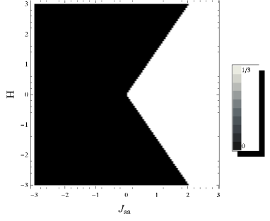
Figure 12: (a) Phase diagram of $a$-sublattice for $|\alpha|=0.025$ and (b) density plot of concurrence $C(\rho)$ versus magnetic field $H$ and coupling constant $J_{aa}$ for $|\alpha|=0.025$ at zero temperature.

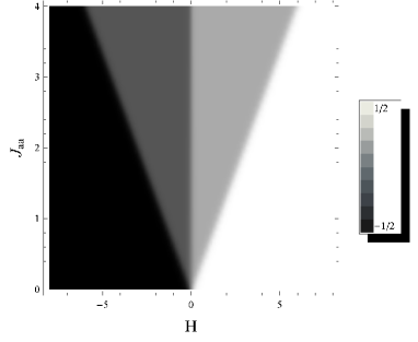
Figure 13: Density plot of magnetization $m_{a}$ versus magnetic field $H$ and coupling constant $J_{aa}$ for $\alpha=0.025$ and $T=0.1$.

6 Conclusion

In this paper we find strong correlations between magnetic properties and quantum entanglement in spin-$\frac{1}{2}$ Ising-Heisenberg model on triangulated Kagomé lattice, which has been proposed to understand a frustrated magnetism of the series of $\mathrm{Cu_{9}X_{2}(cpa)_{6}\cdot nH_{2}O}$ polymeric coordination compounds. The ratio $\alpha=J_{ab}/J_{aa}=0.025$ ($J_{aa}$ labels intra-trimer Heisenberg, while $J_{ab}$ monomer-trimer Ising interactions) is considered, which guaranties experimental realization for suitable theoretical treatment. We adopted variational mean-field like treatment (based on Gibbs-Bogoliubov inequality) of separate clusters in effective interconnected fields of two types (consisting of Heisenberg $a$ trimers and Ising-type $b$ monomers). Each of these fields taken separately describes not only corresponding (a- or b- type) spins, but the whole system.

The calculated magnetic and thermodynamic properties of the model display the (smooth) second order phase transition from ordered into disordered phase driven by temperature and magnetic field. The thermal entanglement properties of $a$-trimers are the central in the aforementioned approximation. Since there are some open questions in the definition of multipartite entanglement (for example, see [64, 65]) we used concurrence as a computable measure of bipartite entanglement for the trimeric units in terms of $XXX$ Heisenberg model in self-consistent magnetic field applied to $a$ subsystem. Due to the classical character of Ising-type interactions the states of two neighboring Heisenberg trimers are separable. Using this fact we studied the entanglement of the each ”$a$ subdivisions” of the cluster individually in effective Ising-type field.Our results show that entanglement does not vanish in zero external field as it happens for the mean field treatment of the isotropic $XXX$ Heisenberg model on triangulated lattice. The geometrical structure of the lattice is responsible for the frustration effects arising in the antiferromagnetic Heisenberg model (geometrical frustration). It leads to existence of magnetization plateaus at $|m_{a}|=1/6$ and concurrence at $C(\rho)=1/3$. Besides the effective field in mean-field solution also depends on the lattice structure (via the number of $b$-sites in the cluster).

In addition, the entangled-disentangled phases in concurrence and order-disordered phases in quantum phase transitions share many common features. The threshold temperature for concurrence is identical to critical temperature of second order phase transition. Besides the entanglement and thermodynamic properties exhibit also common (plateau and peak) behavior in magnetization, susceptibility and concurrence. Moreover, we found that for antiferromagnetic interaction the magnetic susceptibility peaks coincide with the corresponding phase boundaries at which the entanglement vanishes. However, this does not take place for the classical ferromagnetic interaction. This fact allows one to notice a quite visible correlation for the boundaries between various phases for entanglement, susceptibility and magnetization densities as a fingerprints of corresponding quantum phase transitions. Thus, the density diagrams in the presence of magnetic field can be considered as a useful tools to detect important relationships between entanglement-disentanglement transitions in concurrence and corresponding order-disorder quantum phase transitions in quantum magnetism.

7 Acknowledgements

This work was supported by the PS-1981 ANSEF and ECSP-09-08-sasp NFSAT research grants.

References

References

- [1] Misguich G, Lhuillier C 2004, in Frustrated Spin Systems, Diep H T, Ed. (World-Scientific, Singapore), 229-306.
- [2] Lee S-H, Kikuchi H, Qiu Y, Lake B, Huang Q, Habicht K, and Kiefer K 2007 Nature Materials 6 853.
- [3] Moessner R and Sondhi S L 2001 Phys. Rev. B 63 224401.
- [4] Schmidt B, Shannon N, Thalmeier P 2006 J. Phys.: Conf. Ser. 51 207.
- [5] Zhitomirsky M E, Honecker A, Petrenko O A 2000 Phys. Rev. Lett. 85 3269.
- [6] Lee S and Lee K-C 1998 Phys. Rev. B 57 8472.
- [7] Ono T et al 2005 J. Phys. Soc. Japan 74 (Suppl.) 135.
- [8] Narumi Y et al. 2004 Europhys. Lett. 65 705.
- [9] Shastry B S and Sutherland B 1981 Physica B 108 1069.
- [10] Kageyama H et al. 2001 J. Alloy. Compd. 317 177; Kageyama H et al. 2002 Prog. Theor. Phys. Suppl. 145 101.
- [11] Kocharian A N, Fernando G W, Palandage K and Davenport J W 2006 J. Magn. Magn. Mater. 300, e585; Kocharian A N, Fernando G W, Palandage K, and Davenport J W 2006 Phys. Rev. B 74 024511.
- [12] Isaev L, Ortiz G, and Dukelsky J Phys. Rev. Lett. 2009 103, 177201; Dorier J, Schmidt K P, and Mila F 2008 Phys. Rev. Lett. 101, 250402; Japaridze G I, Mahdavifar S 2009 Eur. Phys. J. B 68, 59.
- [13] Hovhannisyan V V, Ananikian N S Phys. Lett. A 2008 372 3363; Ananikyan L N 2007 Int. J. Mod. Phys. B, 21, 755 (2007); Hovhannisyan V V, Ananikyan L N and Ananikian N S 2007 ibid. 20 3567; Arakelyan T A, Ohanyan V R, Ananikyan L N, Ananikian N S, and Roger M 2003 Phys. Rev. B 67 024424; Yao X 2010 Phys. Lett. A, 374 886.
- [14] Kocharian A N, Fernando G W, Palandage K and Davenport J W 2008 Phys. Rev. B 78, 075431 (2008); Nagaoka Y, Phys. Rev. 147, 392 (1966).
- [15] Stone M B, Zaliznyak I, Reich D H et al. 2001 Phys. Rev. B 64 144405.
- [16] Wawrzynska A, Coldea R, Wheeler E M et al. 2008 Phys. Rev. B 77 094439.
- [17] Grohol D, Matan K, Cho J H et al. 2005 Nature Materials 4 323.
- [18] Gardner J S, Gingras M J P, Greedan J E 2010 Rev. Mod. Phys. 82 53.
- [19] Greedan J E 2001 J. Mater. Chem. 11 37; Harrison A 2004 J. Phys.: Condens. Matter 16 S553.
- [20] Norman R E, Rose N J and Stenkamp R E 1987, J. Chem. Soc.: Dalton Trans. 12 2905; Norman R E and Stenkamp R E 1990 Acta Crystallogr. C 46, 6; Gonzalez M, Cervantes-Lee F and Haar L W 1993 Mol. Cryst. Liq. Cryst. 233 317.
- [21] Maruti S and ter Haar L W 1994 J. Appl. Phys. 75 5949; Ateca S, Maruti S, and ter Haar L W 1995 J. Magn. Magn. Mater. 147 398.
- [22] Ramirez A P 2001 in Handbook of Magnetic Materials, K. J. H. Buschow K J H, Ed. (Amsterdam: Elsevier Science), vol. 13, 423-520.
- [23] Strečka J 2007 J. Magn. Magn. Mater. 316 e346.
- [24] Ryo N, Yuichi W, Yuhei N 1997 J. Phys. Soc. Japan 66 3687.
- [25] Zheng J and Sun G 2005 Phys. Rev. B 71 052408.
- [26] Strečka J, Čanova L, Jaščur M, and Hagiwara M 2008 Phys. Rev. B 78 024427.
- [27] Yao D-X, Loh Y L and Carlson E W 2008 Phys. Rev. B 78 024428.
- [28] Mekata M et al. 1998 J. Magn. Magn. Mater. 177 731; Mekata M, Abdulla M, Kubota M, and Oohara Y 2001 Can. J. Phys. 79 1409.
- [29] Amico L, Fazio R, Osterloh A, Vedral V 2008 Rev. Mod. Phys. 80 517; Peschel I and Eisler V 2009 J. Phys. A: Math. Gen. 42 504003; Amico L and Fazio R 2009 ibid. 42 504001; Gühne O, Toth G 2009 Phys. Reports 474 1.
- [30] Bennett C H, DiVincenzo D P, Smolin J A, and Wootters W K 1996 Phys. Rev. A 54 3824; Bennett C H, Brassard G, Crépeau C, Jozsa R, Peres A, and Wootters W K 1993 Phys. Rev. Lett. 70 1895; Bennett C H, Brassard G, Popescu S, Schumacher B, Smolin J A, and Wootters W K 1996 ibid. 76, 722; Ekert A K 1991 ibid. 67 661; 1992 Nature (London) 358 14.
- [31] Arnesen M C, Bose S, and Vedral V 2001 Phys. Rev. Lett. 87 017901.
- [32] Gunlycke D, Kendon V M, Vedral V, and Bose S 2001 Phys. Rev. A 64 042302.
- [33] Wang X 2001 Phys. Rev. A 64 012313; 2001 Phys. Lett. A 281 101.
- [34] Vidal J, Palacios G, and Mosseri R 2004 Phys. Rev. A 69 022107.
- [35] Vidal G, Latorre J I, Rico E, and Kitaev A 2003 Phys. Rev. Lett. 90 227902; Latorre J I, Rico E, and Vidal G 2004 Quantum Inf. Comput. 4 48.
- [36] Larsson D and Johannesson H 2005 Phys. Rev. Lett. 95 196406.
- [37] Yang C, Kocharian A N, and Chiang Y L 2000 J. Phys.: Condens. Matter 12 7433.
- [38] Alba V, Tagliacozzo L, and Calabrese P 2010 Phys. Rev. B 81 060411(R); Calabrese P and Cardy J 2009 J. Phys. A: Math. Gen. 42 504005.
- [39] Souza A M, Reis M S, Soares-Pinto D O et al. 2008 Phys. Rev. B 77 104402.
- [40] Lima Sharma A L and Gomes A M 2008 Europhys. Lett. 84 60003.
- [41] Rappoport T G , Ghivelder L, Fernandes J C et al. 2007 Phys. Rev. B 75 054422.
- [42] Soares-Pinto D O, Souza A M, Sarthour R S et al. 2009 Europhys. Lett. 87 40008.
- [43] Souza A M, Soares-Pinto D O, Sarthour R S et al. 2009 Phys. Rev. B 79 054408.
- [44] Wang X, Fu H and Solomon A I 2001 J. Phys. A: Math. Theor 34 11307.
- [45] Subrahmanyam V 2004 Phys. Rev. A 69 022311.
- [46] See e.g. Mahan G D, Many-Particle Physics (Kluwer/Plenum, New York, 2000); Wen X-G, Quantum Field Theory of Many-Body Systems (OUP, Oxford, 2004); Wei G, Liu J, Miao H, and Du A 2007 Phys. Rev. B 76 054402; Voo K-K 2010 J. Phys.: Condens. Matter 22 275702.
- [47] Gong S-S, Su G 2009 Phys. Rev. A 80 012323; Asoudeh M and Karimipour V 2006 Phys. Rev. A 73 062109; Canosa N, Matera J M, Rossignoli R 2007 Phys. Rev. A 76 022310; Tsyplyatyev O and Loss D 2009 Phys. Rev. A 80 023803.
- [48] Vedral V 2004 New J. Phys. 6 22.
- [49] Hill S and Wootters W K 1997 Phys. Rev. Lett. 78 5022; Wootters W K 1998 Phys. Rev. Lett. 80 2245.
- [50] Bogoliubov N N 1947 J. Phys. (USSR) 11 23; Feynman R P 1955 Phys. Rev. 97 660.
- [51] Kocharian A N, Yang C, Chiang Y L and Chou 2003 Inter. J. Mod. Phys. B 17 5749.
- [52] Pereira M S S, de Moura F A B F and Lyra M L 2008 Phys. Rev. B 77 024402.
- [53] Chaboussant G, Sieber A, Ochsenbein S, Güdel H-U, Murrie M, Honecker A, Fukushima N, Normand B 2004 Phys. Rev. B 70 104422.
- [54] Kou H Z, Zhou B C, Gao S, Liao D-Z, Wang R-J 2003 Inorg. Chem. 42 5604.
- [55] Hagiwara M et al. 2006 Phys. Rev. Lett. 96 147203; Zhitomirsky M E and Honecker A 2004 J. Stat. Mech.: Theor. Exp. P07012; Trippe C, Honecker A, Klumper A and Ohanyan V 2010 Phys. Rev. B 81 054402.
- [56] Antonosyan D, Bellucci S and Ohanyan V 2009 Phys. Rev. B 79 014432.
- [57] Abouie J, Langari A and Siahatgar M 2010 J. Phys.: Condens. Matter 22 216008.
- [58] O’Connor K M and Wootters W K 2001 Phys. Rev. A 63 052302; Wang X. and Zanardi P 2002 Phys. Lett. A 301 1.
- [59] Rau A R P 2009 J. Phys. A: Math. Gen. 42 412002; Rau A R P, Ali M, Alber G 2008 Eur. Phys. Lett. 82 40002.
- [60] Yu T and Eberly J H 2006 Phys. Rev. Lett. 97 140403.
- [61] Wieśniak M, Vedral V and Brukner Č 2005 New J. Phys. 7, 258.
- [62] Maruti S and ter Haar L W, 1993 J. App. Phys. 75 5949.
- [63] Maegawa S, Kaji R, Kanou S, Oyamada A and Nishiyama M 2007 J. Phys.: Condens. Matter 19 145250.
- [64] Barnum H, Knill E, Ortiz G and Viola L 2003 Phys. Rev. A 68 032308; Meyer D A and Wallach N R 2002 J. Math. Phys. 43 4273.
- [65] Wei T C and Goldbart P M 2003 Phys. Rev. A 68 042307.