Did a 1-dimensional magnet detect a 248-dimensional Lie algebra?

Abstract.

About a year ago, a team of physicists reported in Science that they had observed “evidence for ${{\mathsf{E}}_{8}}$ symmetry” in the laboratory. This expository article is aimed at mathematicians and explains the chain of reasoning connecting measurements on a quasi-1-dimensional magnet with a 248-dimensional Lie algebra.

You may have heard some of the buzz spawned by the recent paper [CTW⁺] in Science. That paper described a neutron scattering experiment involving a quasi-one-dimensional cobalt niobate magnet, and led to rumors that ${{\mathsf{E}}_{8}}$ had been detected “in nature”. This is fascinating, because ${{\mathsf{E}}_{8}}$ is a mathematical celebrity and because such a detection seems impossible: it is hard for us to imagine a realistic experiment that could directly observe a 248-dimensional object like ${{\mathsf{E}}_{8}}$.

The connection between the cobalt niobate experiment and ${{\mathsf{E}}_{8}}$ is as follows. Around 1990, physicist Alexander Zamolodchikov and others studied perturbed conformal field theories in general; one particular application of this was a theoretical model describing a 1-dimensional magnet subjected to two magnetic fields. This model makes some numerical predictions which were tested in the cobalt niobate experiment, and the results were as predicted by the model. As the model involves ${{\mathsf{E}}_{8}}$ (in a way we will make precise in §6), one can say that the experiment provides evidence for “${{\mathsf{E}}_{8}}$ symmetry”. No one is claiming to have directly observed ${{\mathsf{E}}_{8}}$.

Our purpose here is to fill in some of the details omitted in the previous paragraph. We should explain that we are writing as journalists rather than mathematicians here, and we are not physicists. We will give pointers to the physics literature so that the adventurous reader can go directly to the words of the experts for complete details.

1. The Ising model

The article in Science describes an experiment involving the magnetic material cobalt niobate (CoNb₂O₆).

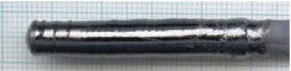
Figure 1. Photograph of an artificially-grown single crystal of CoNb₂O₆. The experiment involved a 2-centimeter-long piece of this crystal, weighing about 8 grams. (Image courtesy of Radu Coldea.)

The material was chosen because the internal crystal structure is such that magnetic Co²⁺ ions are arranged into long chains running along one of the crystal’s axes, and this could give rise to 1-dimensional magnetic behavior. In particular, physicists expected that this material would provide a realization of the famous Ising model, which we now describe briefly.

The term Ising model refers generically to the original, classical model. This simple model for magnetic interactions was suggested by W. Lenz as a thesis problem for his student E. Ising, whose thesis appeared in Hamburg in 1922 [I]. The classical form of the model is built on a square, periodic, $n$-dimensional lattice, with the periods sufficiently large that the periodic boundary conditions don’t play a significant role in the physics. Each site $j$ is assigned a spin $\sigma_{j}=\pm 1$, interpreted as the projection of the spin onto some preferential axis. The energy of a given configuration of spins is

(1.1) $$H=-J\sum_{\langle i,j\rangle}\sigma_{i}\sigma_{j},$$

where $J$ is a constant and the sum ranges over pairs $\langle i,j\rangle$ of nearest-neighbor sites. This Hamiltonian gives rise to a statistical ensemble of states that is used to model the thermodynamic properties of actual magnetic materials. This essentially amounts to a probability distribution on the set of spin configurations, with each configuration weighted by $e^{-kH/T}$ (the Boltzmann distribution), where $k$ is constant and $T$ is the temperature. The assumption of this distribution makes the various physical quantities, such as individual spins, average energy, magnetization, etc., into random variables. For $J>0$, spins at neighboring sites tend to align in the same direction; this behavior is called ferromagnetic, because this is what happens with iron.

To describe the cobalt niobate experiment we actually want the quantum spin chain version of the Ising model. In this quantum model, each site in a 1-dimensional (finite periodic) chain is assigned a 2-dimensional complex Hilbert space. The Pauli spin matrices $S^{x}$, $S^{y}$, and $S^{z}$ act on each of these vector spaces as spin observables, meaning they are self-adjoint operators whose eigenstates correspond to states of particular spin. For example, the $\pm 1$ eigenvectors of $S^{z}$ correspond to up and down spins along the $z$-axis. A general spin state is a unit vector in the 2-dimensional Hilbert space, which could be viewed as a superposition of up and down spin states, if we use those eigenvectors as a basis.

The Hamiltonian operator for the standard 1-dimensional quantum Ising model is given by

(1.2) $$\hat{H}=-K\sum_{j}\Bigl{[}S^{z}_{j}S^{z}_{j+1}+g_{x}S^{x}_{j}\Bigr{]}.$$

In the quantum statistical ensemble one assigns probabilities to the eigenvectors of $\hat{H}$ weighted by the corresponding energy eigenvalues. This then defines, via the Boltzmann distribution again, a probability distribution on the unit ball in the total Hilbert space of the system.

Just as in the classical case, physical quantities become random variables with distributions that depend on the temperature and constants $K$ and $g_{x}$. It is by means of these distributions that the model makes predictions about the interrelationships of these quantities.

The first term in the Hamiltonian (1.2) has a ferromagnetic effect (assuming $K>0$), just as in the classical case. That is, it causes spins of adjacent sites to align with each other along the $z$-axis, which we will refer to as the preferential axis. (Experimental physicists might call this the “easy” axis.) The second term represents the influence of an external magnetic field in the $x$-direction, perpendicular to the $z$-direction—we’ll refer to this as the transverse axis. The effect of the second term is paramagnetic, meaning that it encourages the spins to align with the transverse field.

The 1-dimensional quantum Ising spin chain exhibits a phase transition at zero temperature. The phase transition (also called a critical point) is the point of transition between the ferromagnetic regime ($g_{x}<1$, where spins tend to align along the $z$-axis) and the paramagnetic ($g_{x}>1$). The critical point $(g_{x}=1)$ is distinguished by singular behavior of various macroscopic physical quantities, such as the correlation length. Roughly speaking, this is the average size of the regions in which the spins are aligned with each other.

To define correlation length a little more precisely, we consider the statistical correlation between the $z$-components of spins at two sites separated by a distance $r$. These spins are just random variables whose joint distribution depends on the constants $K$ and $g_{x}$ as well as the separation $r$ and the temperature $T$. (We are assuming $r$ is large compared to the lattice spacing, but small compared to the overall dimensions of the system.) For $g_{x}>1$ the correlation falls off exponentially as $e^{-r/\xi}$, because spins lined up along the $x$-axis will be uncorrelated in the $z$-direction; the constant $\xi$ is the correlation length. In contrast, at the critical point $g_{x}=1$ and $T=0$, the decay of the spin correlation is given by a power law; this radical change of behavior corresponds to the divergence of $\xi$. This phase transition has been observed experimentally in a LiHoF₄ magnet [BRA].

One might wonder why an external magnetic field is included by default in the quantum case but not in the classical case. The reason for this is a correspondence between the classical models and the quantum models of one lower dimension. The quantum model includes a notion of time-evolution of an observable according to the Schrödinger equation, and the correspondence involves interpreting one of the classical dimensions as imaginary time in the quantum model. Under this correspondence, the classical interaction in the spatial directions gives the quantum ferromagnetic term, while interactions in the imaginary time direction give the external field term, see [Sa, §2.1.3] for details.

Although there are some important differences in the physical interpretation on each side, the classical-quantum correspondence allows various calculations to be carried over from one case to the other. For example, the critical behavior of the 1-dimensional transverse-field quantum Ising model (1.2) at zero temperature, with the transverse field parameter tuned to the critical value $g_{x}=1$, can be “mapped” onto equivalent physics for the classical 2-dimensional Ising model (1.1), at a non-zero temperature. The latter case is the famous phase transition of the 2-dimensional classical model, which was discovered by Peierls and later solved exactly by Onsager [O].

2. Adapting the model to the magnet

The actual magnet used in the experiment is not quite modeled by the quantum Ising Hamiltonian (1.2). In the ferromagnetic regime ($g_{x}<1$), weak couplings between the magnetic chains create an effective magnetic field pointing along the preferential axis [CT]. The relevant model for the experiment is thus

(2.1) $$\hat{H}=-K\sum_{j}\Bigl{[}S^{z}_{j}S^{z}_{j+1}+g_{x}S^{x}_{j}+g_{z}S^{z}_{j}\Bigr{]},$$

which is just (1.2) with an additional term $g_{z}S^{z}_{j}$ representing this internal magnetic field.

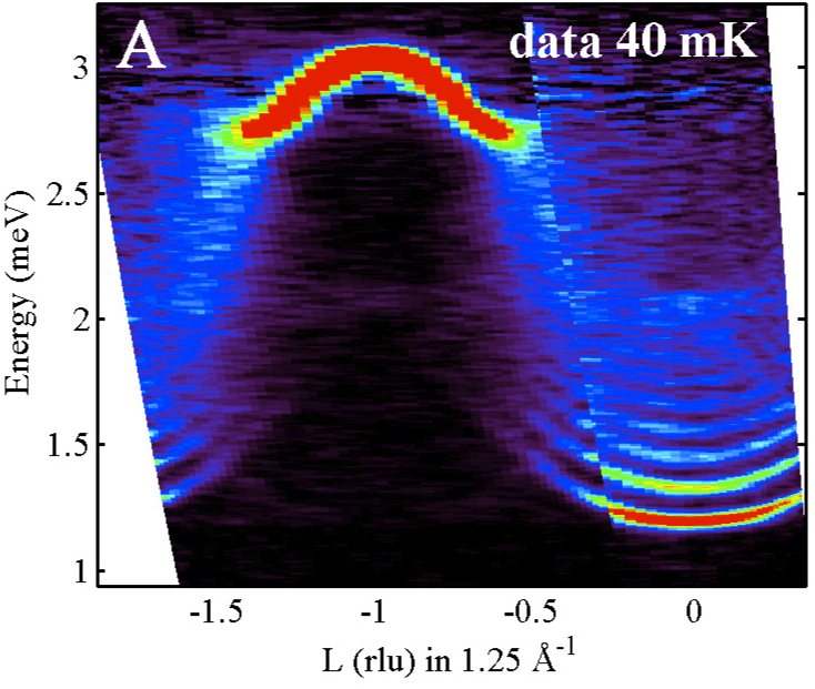
(A) Experimental data at 40mK

(B) Calculated

Figure 2. Comparison of excitations under no external magnetic field: experimental (left) versus predictions based on the 1-dimensional model (right). (Figure adapted from [CTW⁺].)

The first phase of the cobalt niobate experiment tested the appropriateness of (2.1) as a model for the magnetic dynamics in the absence of an external magnetic field, i.e., with $g_{x}=0$. The experimental evidence does support the claim that this 3-dimensional object is behaving as a 1-dimensional magnetic system. For example, Figure 2 shows a comparison of the experimental excitation energies (as a function of wave vector) to theoretical predictions from the 1-dimensional model. The presence of a sequence of well-defined and closely spaced energy levels, as shown in these pictures, is predicted only in dimension one.

3. What is ${{\mathsf{E}}_{8}}$?

Before we explain how the rather simple quantum Ising model from the previous sections leads to a theory involving ${{\mathsf{E}}_{8}}$, we had better nail down what it means to speak of “${{\mathsf{E}}_{8}}$”. It’s an ambiguous term, with at least the following six common meanings:

1. The root system of type ${{\mathsf{E}}_{8}}$. This is a collection of 240 points, called roots, in $\mathbb{R}^{8}$. The usual publicity photo for ${{\mathsf{E}}_{8}}$ (reproduced in Figure 3A) is the orthogonal projection of the root system onto a copy of $\mathbb{R}^{2}$ in $\mathbb{R}^{8}$.

2. The ${{\mathsf{E}}_{8}}$ lattice, which is the subgroup of $\mathbb{R}^{8}$ (additively) generated by the root system.

3. A complex Lie group—in particular, a closed subgroup of $\operatorname{GL}_{248}(\mathbb{C})$—that is simple and 248-dimensional.

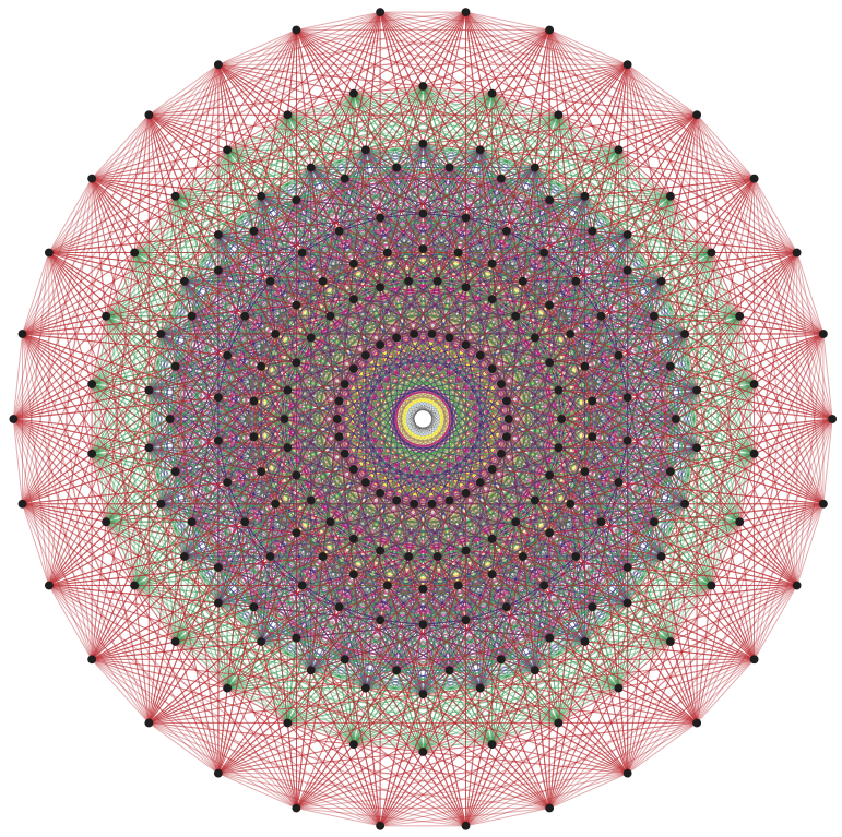
(A) The popular picture

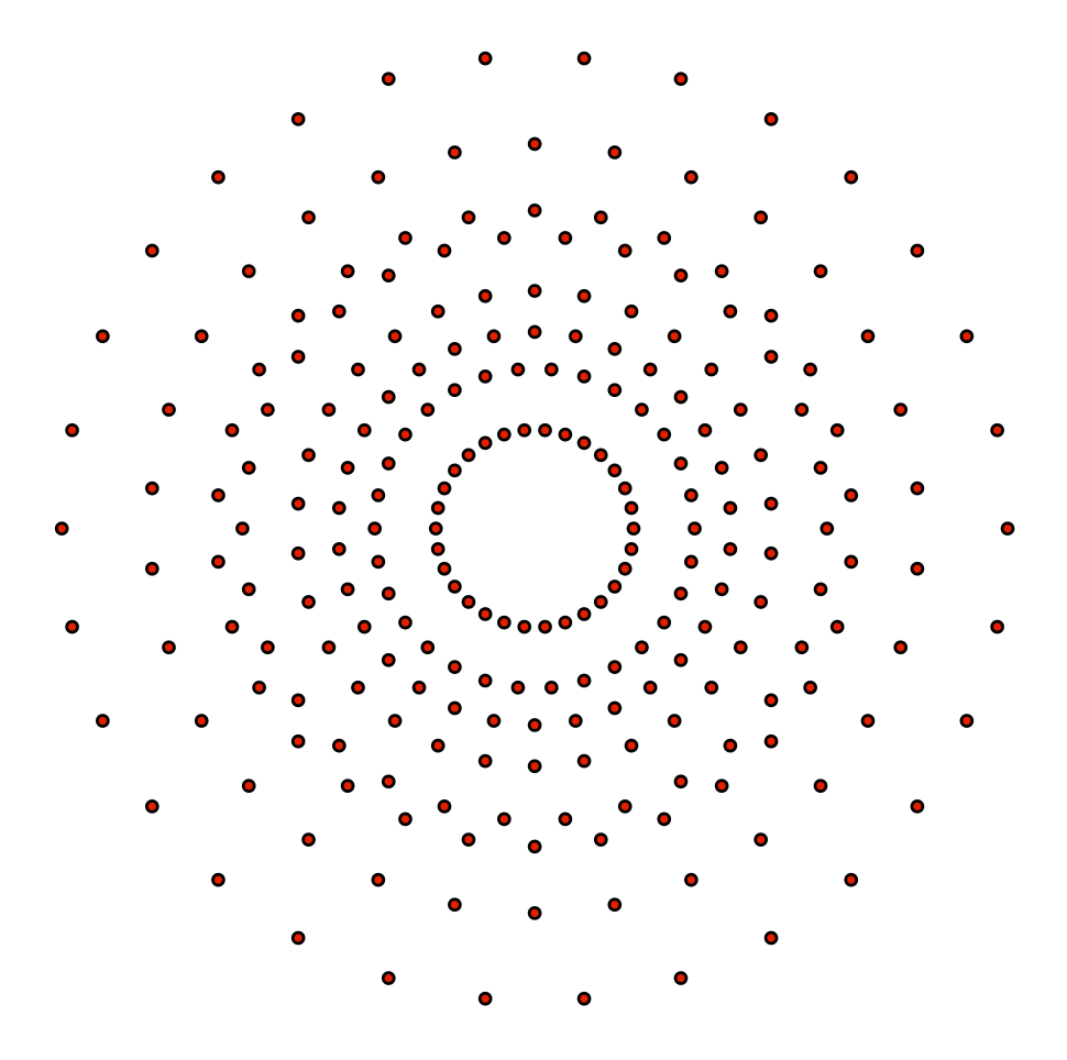
(B) Vertices only

Figure 3. The left panel (A) is the picture of ${{\mathsf{E}}_{8}}$ that one finds in the popular press. Deleting some edges leaves you with the frontispiece of [Cox]. (Image courtesy of John Stembridge [St].) The right panel (B) is the same picture with the edges removed; it is the image of the root system of ${{\mathsf{E}}_{8}}$ in a Coxeter plane.

There are also three simple real Lie groups—meaning in particular that they are closed subgroups of $\operatorname{GL}_{248}(\mathbb{R})$—whose complexification is the complex Lie group from (3). (The fact that there are exactly three is part of Elie Cartan’s classification of simple real Lie groups; see [Se 02, §II.4.5] for an outline of a modern proof.) They are:

1. The split real ${{\mathsf{E}}_{8}}$. This is the form of ${{\mathsf{E}}_{8}}$ that one can define easily over any field or even over an arbitrary scheme. Its Killing form has signature 8.

2. The compact real ${{\mathsf{E}}_{8}}$, which is the unique largest subgroup of the complex ${{\mathsf{E}}_{8}}$ that is compact as a topological space. Its Killing form has signature $-248$.

3. The remaining real form of ${{\mathsf{E}}_{8}}$ is sometimes called “quaternionic”. Its Killing form has signature $-24$.

In physics, the split real ${{\mathsf{E}}_{8}}$ appears in supergravity [MS] and the compact real ${{\mathsf{E}}_{8}}$ appears in heterotic string theory [GHMR]. These two appearances in physics, however, are purely theoretical; the models in which they are appear are not yet subject to experiment. It is the compact real ${{\mathsf{E}}_{8}}$ (or, more precisely, the associated Lie algebra) that appears in the context of the cobalt niobate experiment, making this the first actual experiment to detect a phenomenon that could be modeled using ${{\mathsf{E}}_{8}}$.

There have also been two recent frenzies in the popular press concerning ${{\mathsf{E}}_{8}}$. One concerned the computation of the Kazhdan-Lusztig-Vogan polynomials which you can read about in the prizewinning paper [V]; that work involved the split real ${{\mathsf{E}}_{8}}$. The other frenzy was sparked by the manuscript [L]. The ${{\mathsf{E}}_{8}}$ referred to in [L] is clearly meant to be one of the real forms, but the manuscript contains too many contradictory statements to be sure which one, and in any case the whole idea has serious difficulties as explained in [DG10].

Groups versus algebras

Throughout this note we conflate a real Lie group $G$, which is a manifold, with its Lie algebra $\mathfrak{g}$, which is the tangent space to $G$ at the identity and is a real vector space endowed with a nonassociative multiplication. This identification is essentially harmless and is standard in physics. Even when physicists discuss symmetry “groups”, they are frequently interested in symmetries that hold only in a local sense, and so the Lie algebra is actually the more relevant object.

Real versus complex

Moreover, physicists typically compute within the complexification $\mathfrak{g}\otimes\mathbb{C}$ of $\mathfrak{g}$. This is the complex vector space with elements of the form $sx+ity$ for $s,t\in\mathbb{R}$ and $x,y\in\mathfrak{g}$, where complex conjugation acts via $sx+ity\mapsto sx-ity$. Note that one can recover $\mathfrak{g}$ as the subspace of elements fixed by complex conjugation. Therefore, morally speaking, working with the $\mathbb{R}$-algebra $\mathfrak{g}$ (as mathematicians often do) amounts to the same as working with $\mathfrak{g}\otimes\mathbb{C}$ together with complex conjugation (as physicists do). This is an example of the general theory of Galois descent as outlined in, e.g., [J 79, §X.2] or [Se 79, §X.2].

4. From the Ising model to ${{\mathsf{E}}_{8}}$

What possible relevance could a 248-dimensional algebra have for a discrete one-dimensional statistical physics model? This is a long and interesting story, and we can only give a few highlights here.

As we mentioned above, the 1-dimensional quantum Ising model from (1.2) undergoes a phase transition at zero temperature at the critical value of the transverse magnetic field strength. If the system is close to this critical point, the correlation length (described in §1) will be very large compared to the lattice spacing, and so we can assume that the discrete spins vary smoothly across nearby lattice sites. In this regime we can thus effectively model the system using continuous “field” variables, i.e., using quantum field theory. For the 1-dimensional quantum Ising model, the corresponding continuous theory is a quantum field theory of free, spinless fermionic particles in 1+1 space-time dimensions.

To understand what happens as the critical point is approached, one can apply “scaling” transformations that dilate the macroscopic length scales (e.g. the correlation length) while keeping the microscopic lengths (e.g. the lattice spacing) unchanged. (See, e.g., [Sa, §4.3] for a more thorough explanation of this.) The limiting theory at the critical point should then appear as a fixed point for these transformations, called the scaling limit. Polyakov famously argued in [P] that the scaling limit should be distinguished by invariance with respect to local conformal transformations. This paper established the link between the study of phase transitions and conformal field theory (CFT).

In [BPZ], Belavin, Polyakov, and Zamolodchikov showed that certain simple CFT’s called minimal models could be solved completely in terms of (and so are determined by) a Hilbert space made of a finite number of “discrete series” (unitary, irreducible) representations of the Virasoro algebra, see [He, Chap. 2] or [DFMS, Chap. 7] for more details. These representations are characterized by the eigenvalue $c$ assigned to the central element, called the central charge, which can be computed directly from the scaling limit of the statistical model. This works out beautifully in the case of the critical 1-dimensional quantum Ising model: In that case, the central charge is $c=1/2$, the minimal model is built from the three discrete series representations of the Virasoro algebra with that central charge, and this CFT exactly matches the Ising phase transition, see [BPZ, App. E], [DFMS, §7.4.2], or [Mu, §14.2] for details.

The discrete series representations mentioned above are described by $c$ and another parameter $h$ which have some relations between them, and there are tight constraints on the possible values of $c$ and $h$ to be unitary [FQS]. To prove that all of these values of $c$ and $h$ indeed correspond to irreducible unitary representations, one employs the coset construction of Goddard, Kent, and Olive, see [GKO] or [DFMS, Chap. 18]. This construction produces such representations by restricting representations of an affine Lie algebra, i.e., a central extension of the (infinite-dimensional) loop algebra of a compact Lie algebra $\mathfrak{g}$. Using the coset construction, there are two ways to obtain the $c=1/2$ minimal model that applies to our zero-field Ising model: we could use either of the compact Lie algebras $\mathfrak{su}(2)$ or ${{\mathsf{E}}_{8}}$ as the base $\mathfrak{g}$ for the affine Lie algebra [DFMS, §18.3, §18.4.1]. These two algebras are the only choices that lead to $c=1/2$ [Mu, §14.2].

Of course, the appearance of ${{\mathsf{E}}_{8}}$ here is somewhat incidental. The minimal model could be described purely in terms of Virasoro representations, without reference to either $\mathfrak{su}(2)$ or ${{\mathsf{E}}_{8}}$. As we explain below, ${{\mathsf{E}}_{8}}$ only takes center stage when we consider a perturbation of the critical Ising model as in (2.1).

5. Magnetic perturbation and Zamolodchikov’s calculation

In a 1989 article [Z], Zamolodchikov investigated the field theory for a model equivalent to the 1-dimensional quantum Ising model (1.2), in the vicinity of the critical point, but perturbed by a small magnetic field directed along the preferential spin axis. In other words, he considered the field theory model corresponding to (2.1) with $g_{x}\approx 1$ and $g_{z}$ very small. Note the change of perspective: for Zamolodchikov $g_{x}$ is fixed and the perturbation consists of a small change in the value of $g_{z}$. But in the cobalt niobate experiment, this magnetic “perturbation” is already built-in—it is the purely internal effect arising from the inter-chain interactions as we described in §2. The experimenters can’t control the strength of the internal field, they only vary $g_{x}$. Fortunately, the internal magnetic field $g_{z}$ turns out to be relatively weak, so when the external field $g_{x}$ is tuned close to the critical value the experimental model matches the situation considered by Zamolodchidkov.

The qualitative features of the particle spectrum for the magnetically perturbed Ising model had been predicted by McCoy and Wu [MW 78]. Those earlier calculations show a large number of stable particles for small $g_{x}$, with the number decreasing as $g_{x}$ approaches $1$. Zamolodchikov’s paper makes some predictions for the masses of these particles at $g_{x}=1$.

As we noted above, the $c=1/2$ minimal model is the conformal field theory associated with the phase transition of the unperturbed quantum Ising model. The perturbed field theory is no longer a conformal field theory, but Zamolodchikov found six local integrals of motion for the perturbed field theory and conjectured that these were the start of an infinite series. On this basis, he made the fundamental conjecture:

1. The perturbation gives an integrable field theory.

One implication of (Z1) is that the resulting scattering theory should be “purely elastic,” meaning that the number of particles and their individual momenta would be conserved asymptotically. Zamolodchikov combined this purely elastic scattering assumption with three rather mild assumptions on the particle interactions of the theory [Z, p. 4236]:

1. There are at least 2 particles, say $p_{1}$ and $p_{2}$.

2. Both $p_{1}$ and $p_{2}$ appear as bound-state poles on the scattering amplitude for two $p_{1}$’s.

3. The particle $p_{1}$ appears as a bound-state pole in the scattering amplitude between $p_{1}$ and $p_{2}$.

Assumptions (Z3) and (Z4) merely assert that certain coupling constants that govern the interparticle interactions are non-zero, so they could be viewed as an assumption of some minimum level of interaction between the two particles.

The word “particle” bears some explaining here, because it is being used here in the sense of quantum field theory: a stable excitation of the system with distinguishable particle-like features such as mass and momentum. However, it is important to note that the continuum limit of the Ising model is made to look like a field theory only through the application of a certain transformation (Jordan-Wigner, see [Sa, §4.2]), that makes “kink” states (boundaries between regions of differing spin) the basic objects of the theory. So Zamolodchikov’s particles aren’t electrons or ions. The field theory excitations presumably correspond to highly complicated aggregate spin states of the original system. On the statistical physics side the usual term for this kind of excitation is quasiparticle. In the experiment these quasiparticles are detected just as ordinary particles would be, by measuring the reaction to a beam of neutrons.

From the mild assumptions (Z2)–(Z4), he showed that the simplest purely elastic scattering theory consistent with the integrals of motion contains 8 particles with masses listed in Table 1. (See [He, §14.3] for more background on these calculations.) These predictions were quickly corroborated by computational methods, through numerical diagonalization of the Hamiltonian (2.1), see [HeS] or [SZ]. In Table 1, $m_{1}$ and $m_{2}$ are the masses of the two original particles $p_{1}$ and $p_{2}$. Note that only the ratios of the masses, such as $m_{2}/m_{1}$, are predicted; in the discrete model (2.1) the individual masses would depend on the overall length of the lattice, and in passing to the scaling limit we give up this information.

$$\begin{array}[]{c@{\ =\ }c@{\ \approx\ }c}m_{2}&2\cos\frac{\pi}{5}m_{1}&1.618m_{1}\\[2.15277pt] m_{3}&2\cos\frac{\pi}{30}m_{1}&1.989m_{1}\\[2.15277pt] m_{4}&2\cos\frac{\pi}{5}\cos\frac{7\pi}{30}m_{1}&2.405m_{1}\\[2.15277pt] m_{5}&4\cos\frac{\pi}{5}\cos\frac{2\pi}{15}m_{1}&2.956m_{1}\\[2.15277pt] m_{6}&4\cos\frac{\pi}{5}\cos\frac{\pi}{30}m_{1}&3.218m_{1}\\[2.15277pt] m_{7}&8(\cos\frac{\pi}{5})^{2}\cos\frac{7\pi}{30}m_{1}&3.891m_{1}\\[2.15277pt] m_{8}&8(\cos\frac{\pi}{5})^{2}\cos\frac{2\pi}{15}m_{1}&4.783m_{1}\end{array}$$

Table 1. The masses of the particles predicted by Zamolodchikov.

Zamolodchikov’s results give some indications of a connection with the algebra or root system ${{\mathsf{E}}_{8}}$. The spins of the six integrals of motion he calculated were

$$s=1,7,11,13,17,19.$$

The conjecture is that this is the start of a sequence of integrals of motion whose spins include all values of $s$ relatively prime to $30$. These numbers are suggestive because 30 is the Coxeter number of ${{\mathsf{E}}_{8}}$ and the remainders of these numbers modulo 30 are the exponents of ${{\mathsf{E}}_{8}}$ (see for example [Bo] for a definition of Coxeter number and exponent). This was taken as a hint that the conjectured integrable field theory could have a model based on ${{\mathsf{E}}_{8}}$, and in fact such a connection with ${{\mathsf{E}}_{8}}$ had already been conjectured by Fateev based on other theoretical considerations [Z, p. 4247, 4248].

6. Affine Toda field theory

Soon after Zamolodchikov’s first paper appeared, Fateev and Zamolodchikov conjectured in [FZ] that if you take a minimal model CFT constructed from a compact Lie algebra $\mathfrak{g}$ via the coset construction and perturb it in a particular way, then you obtain the affine Toda field theory (ATFT) associated with $\mathfrak{g}$, which is an integrable field theory. This was confirmed in [EY] and [HoM].

If you do this with $\mathfrak{g}={{\mathsf{E}}_{8}}$, you arrive at the conjectured integrable field theory investigated by Zamolodchikov and described in the previous paragraph. That is, if we take the ${{\mathsf{E}}_{8}}$ ATFT as a starting point, then the assumptions (Z1)–(Z4) become deductions. This is the essential role of ${{\mathsf{E}}_{8}}$ in the numerical predictions relevant to the cobalt niobate experiment. (In the next section, we will explain how the masses that Zamolodchikov found arise naturally in terms of the algebra structure. But that is just a bonus.)

What is the role of ${{\mathsf{E}}_{8}}$ in the affine Toda field theory?

To say the ATFT in question is “associated” with ${{\mathsf{E}}_{8}}$ leaves open a range of possible interpretations, so we should spell out precisely what this means. The ATFT construction from a compact Lie algebra $\mathfrak{g}$ proceeds by choosing a Cartan subalgebra $\mathfrak{h}$ in $\mathfrak{g}$—it is a real inner product space with inner product the Killing form $(\,,\,)$, and is isomorphic to $\mathbb{R}^{8}$ in the case $\mathfrak{g}={{\mathsf{E}}_{8}}$. Let $\phi$ be a scalar field in 2-dimensional Minkowski space-time, taking values in $\mathfrak{h}$. Then the Lagrangian density for the affine Toda field theory is

(6.1) $$\frac{1}{2}(\partial_{\mu}\phi,\partial^{\mu}\phi)-(e^{\beta\phi}Ee^{-\beta\phi},\overline{E}),$$

where $\beta$ is a coupling constant. Here $E$ is a regular semisimple element of $\mathfrak{g}\otimes\mathbb{C}$ that commutes with its complex conjugate $\overline{E}$. More precisely, for $x\in\mathfrak{h}$ a principal regular element, conjugation by $e^{2\pi ix/h}$ with $h$ the Coxeter number of $\mathfrak{g}$ gives a $\mathbb{Z}/h$-grading on $\mathfrak{g}\otimes\mathbb{C}$, and the element $E$ belongs to the $e^{2\pi i/h}$-eigenspace. (Said differently, the centralizer of $E$ is a Cartan subalgebra of $\mathfrak{g}\otimes\mathbb{C}$ in apposition to $\mathfrak{h}\otimes\mathbb{C}$ in the sense of [K 59, p. 1018].)

The structure of ${{\mathsf{E}}_{8}}$ thus enters into the basic definitions of the fields and their interactions. However, ${{\mathsf{E}}_{8}}$ does not act by symmetries on this set of fields.

Why is it ${{\mathsf{E}}_{8}}$ that leads to Zamolodchikov’s theory?

We opened this section by asserting that perturbing a minimal model CFT constructed from $\mathfrak{g}$ via the coset construction leads to an ATFT associated with $\mathfrak{g}$. For this association to make sense, the perturbing field is required to have “conformal dimension” $2/(h+2)$. The two coset models for the Ising model give us two possible perturbation theories. Starting from $\mathfrak{su}(2)$, which has $h=2$, we could perturb using the field of conformal dimension $1/2$, which is the energy. This perturbation amounts to raising the temperature away from zero, which falls within the traditional framework of the Ising model and is well-understood.

The other choice is to start from ${{\mathsf{E}}_{8}}$, which has $h=30$, and perturb using the field of conformal dimension $1/16$, which is the magnetic field along the preferential axis. This is exactly the perturbation that Zamolodchikov considered in his original paper. This means that if an ATFT is used to describe the magnetically perturbed Ising model, we have no latitude in the choice of a Lie algebra: it must be ${{\mathsf{E}}_{8}}$.

Why is it the compact form of ${{\mathsf{E}}_{8}}$?

As Folland noted recently in [Fo] physicists tend to think of Lie algebras in terms of generators and relations, without even specifying a background field if they can help it. So it can be difficult to judge from the appearance of a Lie algebra in the physics literature if any particular form of the algebra is being singled out.

Nevertheless, the algebras appearing here are the compact ones. The reason is that the minimal model CFT’s involve unitary representations of the Virasoro algebra. The coset construction shows that these come from representations of affine Lie algebras which are themselves constructed from compact finite-dimensional algebras. And it is these finite-dimensional Lie algebras that appear in the ATFT.

What about ${{\mathsf{E}}_{6}}$ and ${{\mathsf{E}}_{7}}$?

So far, we have explained why it is ${{\mathsf{E}}_{8}}$ that is related to the cobalt niobate experiment. This prompts the question: given a simple compact real Lie algebra $\mathfrak{g}$, does it give a theory describing some other physical setup? Or, to put it differently, what is the physical setup that corresponds to a theoretical model involving, say, ${{\mathsf{E}}_{6}}$ or ${{\mathsf{E}}_{7}}$? In fact, the field theories based on these other algebras do have interesting connections to statistical models. For example, ${{\mathsf{E}}_{7}}$ Toda field theory describes the thermal perturbation of the tricritical Ising model, and the ${{\mathsf{E}}_{6}}$ theory the thermal deformation of the tricritical three-state Potts model. These other models are easily distinguished from the magnetically perturbed Ising model by their central charges. It will be interesting to see if physicists can come up with ways to probe these other models experimentally. The ${{\mathsf{E}}_{7}}$ model might be easiest—the unperturbed, CFT version has already been realized, for example, in the form of helium atoms on krypton-plated graphite [TFV].

7. The Zamolodchikov masses and ${{\mathsf{E}}_{8}}$’s publicity photo

Translating Zamolodchikov’s theory into the language of affine Toda field theory provides a way to transform his calculation of the particle masses listed in Table 1 into the solution of a rather easy system of linear equations, and that in turn is connected to the popular image of the ${{\mathsf{E}}_{8}}$ root system from Figure 3A. These are connections that work for a general ATFT, and we write in that level of generality.

An ATFT is based on a compact semisimple real Lie algebra $\mathfrak{g}$, such as the Lie algebra of the compact real ${{\mathsf{E}}_{8}}$. We assume further that this algebra is simple and is not $\mathfrak{su}(2)$. Then from $\mathfrak{g}$ we obtain a simple root system $R$ spanning $\mathbb{R}^{\ell}$ for some $\ell\geq 2$; this is canonically identified with the dual $\mathfrak{h}^{*}$ of the Cartan subalgebra mentioned at the end of the previous section.

We briefly explain how to make a picture like Figure 3B for $R$. (For background on the vocabulary used here, please see [Bo] or [Ca].) Pick a set $B$ of simple roots in $R$. For each $\beta\in R$, write $s_{\beta}$ for the reflection in the hyperplane orthogonal to $\beta$. The product $w:=\prod_{\beta\in B}s_{\beta}$ with respect to any fixed ordering of $B$ is called a Coxeter element and its characteristic polynomial has $m(x):=x^{2}-2\cos(2\pi/h)x+1$ as a simple factor [Bo, VI.1.11, Prop. 30], where $h$ is the Coxeter number of $R$. The primary decomposition theorem gives a uniquely determined plane $P$ in $\mathbb{R}^{\ell}$ on which $w$ restricts to have minimal polynomial $m(x)$, i.e., is a rotation through $2\pi/h$—we call $P$ the Coxeter plane for $w$. The picture in Figure 3B is the image of $R$ under the orthogonal projection $\pi\!:\mathbb{R}^{\ell}\rightarrow P$ in the case where $R={{\mathsf{E}}_{8}}$. We remark that while $P$ depends on the choice of $w$, all Coxeter elements are conjugate under the orthogonal group [Ca, 10.3.1], so none of the geometric features of $\pi(R)$ are changed if we vary $w$ and we will refer to $P$ as simply a Coxeter plane for $R$.

In Figure 3B, the image of $R$ lies on 8 concentric circles. This is a general feature of the projection in $P$ and is not special to the case $R={{\mathsf{E}}_{8}}$. Indeed, the action of $w$ partitions $R$ into $\ell$ orbits of $h$ elements each [Bo, VI.1.11, Prop. 33(iv)], and $w$ acts on $P$ as a rotation. So the image of $R$ necessarily lies on $\ell$ circles.

The relationship between the circles in Figure 3B and physics is given by the following theorem.

Theorem 7.1.

Let $\mathfrak{g}$ be a compact simple Lie algebra that is not $\mathfrak{su}(2)$, and write $R$ for its root system. For an affine Toda field theory constructed from $\mathfrak{g}$, the following multisets are the same, up to scaling by a positive real number:

1. The (classical) masses of the particles in the affine Toda theory.

2. The radii of the circles containing the projection of $R$ in a Coxeter plane.

3. The entries in a Perron-Frobenius eigenvector for a Cartan matrix of $R$.

The terms in (3) may need some explanation. The restriction of the inner product on $\mathbb{R}^{\ell}$ to $R$ is encoded by an $\ell$-by-$\ell$ integer matrix $C$, called the Cartan matrix of $R$. You can find the matrix for $R={{\mathsf{E}}_{8}}$ in Figure 4A. We know a lot about the Cartan matrix, no matter which $R$ one chooses—for example, its eigenvalues are all real and lie in the interval $(0,4)$, see [BLM, Th. 2]. Further, the matrix $2-C$ has all non-negative entries and is irreducible in the sense of the Perron-Frobenius Theorem, so its largest eigenvalue—hence the smallest eigenvalue of $C$—has a 1-dimensional eigenspace spanned by a vector $\vec{x}$ with all positive entries. (Such an eigenvector is exhibited in Figure 4B for the case $R={{\mathsf{E}}_{8}}$.) This $\vec{x}$ is the vector in (3) and it is an eigenvector of $C$ with eigenvalue $4\sin^{2}(\pi/2h)$, so calculating $\vec{x}$ amounts to solving an easy system of linear equations.

$\left(\begin{matrix}2&0&-1&0&0&0&0&0\\ 0&2&0&-1&0&0&0&0\\ -1&0&2&-1&0&0&0&0\\ 0&-1&-1&2&-1&0&0&0\\ 0&0&0&-1&2&-1&0&0\\ 0&0&0&0&-1&2&-1&0\\ 0&0&0&0&0&-1&2&-1\\ 0&0&0&0&0&0&-1&2\end{matrix}\right)$

(A)

$\left(\begin{matrix}m_{2}\\ m_{4}\\ m_{6}\\ m_{8}\\ m_{7}\\ m_{5}\\ m_{3}\\ m_{1}\end{matrix}\right)$

(B)

Figure 4. The Cartan matrix (A) for the root system ${{\mathsf{E}}_{8}}$ and a Perron-Frobenius eigenvector (B), where the entries are as in Table 1.

Sketch of proof.

Theorem 7.1 has been known to physicists since the early 1990s; here is a gloss of the literature. Freeman showed that (1) and (3) are equivalent in [Fr]. We omit his argument, which amounts to computations in the complex Lie algebra $\mathfrak{g}\otimes\mathbb{C}$, but it is worth noting that his proof does rely on $\mathfrak{g}$ being compact.

The equivalence of (2) and (3) can be proved entirely in the language of root systems and finite reflection groups, see for example [FLO] or [Cor, §2]. The Dynkin diagram (a graph with vertex set $B$) is a tree, so it has a 2-coloring $\sigma\!:B\rightarrow\{\pm 1\}$, and one picks $w$ to be a corresponding Coxeter element as in [Ca, §10.4]. Conveniently, the elements $\sigma(\beta)\beta$ for $\beta\in B$ are representatives of the orbits of $w$ on $R$, see [K 85, p.250, (6.9.2)] or [FLO, p. 91]. It is elementary to find the inner products of $\pi(\sigma(\beta)\beta)$ with the basis vectors for $P$ given in [Ca, §10.4], hence the radius of the circle containing $\pi(\sigma(\beta)\beta)$. The entries of the Perron-Frobenius eigenvector appear naturally, because these entries are part of the expressions for the basis vectors for $P$.

Alternatively, Kostant shows the equivalence of (1) and (2) in [K 10] using Lie algebras. ∎

There is a deeper connection between the particles in the ATFT and the roots in the root system. Physicists identify the $w$-orbits in the root system with particles in the ATFT. The rule for the coupling of particles in a scattering experiment (called a “fusing” rule) is that the scattering amplitude for two particles $\Omega_{1}$ and $\Omega_{2}$ has a bound-state pole corresponding to $\Omega_{3}$ if and only if there are roots $\rho_{i}\in\Omega_{i}$ so that $\rho_{1}+\rho_{2}+\rho_{3}=0$ in $\mathbb{R}^{\ell}$, see [Do] and [FLO]. This leads to a “Clebsch-Gordan” necessary condition for the coupling of particles, see [Br]. We remark that these fusing rules are currently only theoretical—it is not clear how they could be tested experimentally.

8. Back to the experiment

Let’s get back to the cobalt niobate experiment. As we noted above, when the external magnetic field is very close to the critical value that induces the phase transition, it was expected that the experimental system would be modeled by the critical 1-dimensional quantum Ising model perturbed by a small magnetic field directed along the preferential axis. This model is the subject of Zamolodchikov’s perturbation theory, and the resulting field theory has been identified as the ${{\mathsf{E}}_{8}}$ ATFT.

To test this association, the experimenters conducted neutron scattering experiments on the magnet. Figure 5A shows an intensity plot of scattered neutrons averaged over a range of scattering angles. Observations were actually made at a series of external field strengths, from 4.0 tesla (T) to 5.0 T, with the second peak better resolved at the lower energies. Both peaks track continuously as the field strength is varied. Figure 5A represents the highest field strength at which the second peak could be resolved.

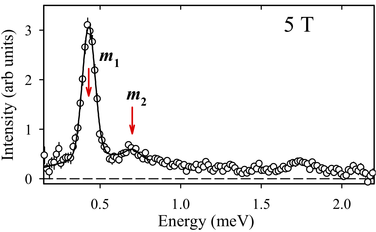
(A) Masses detected

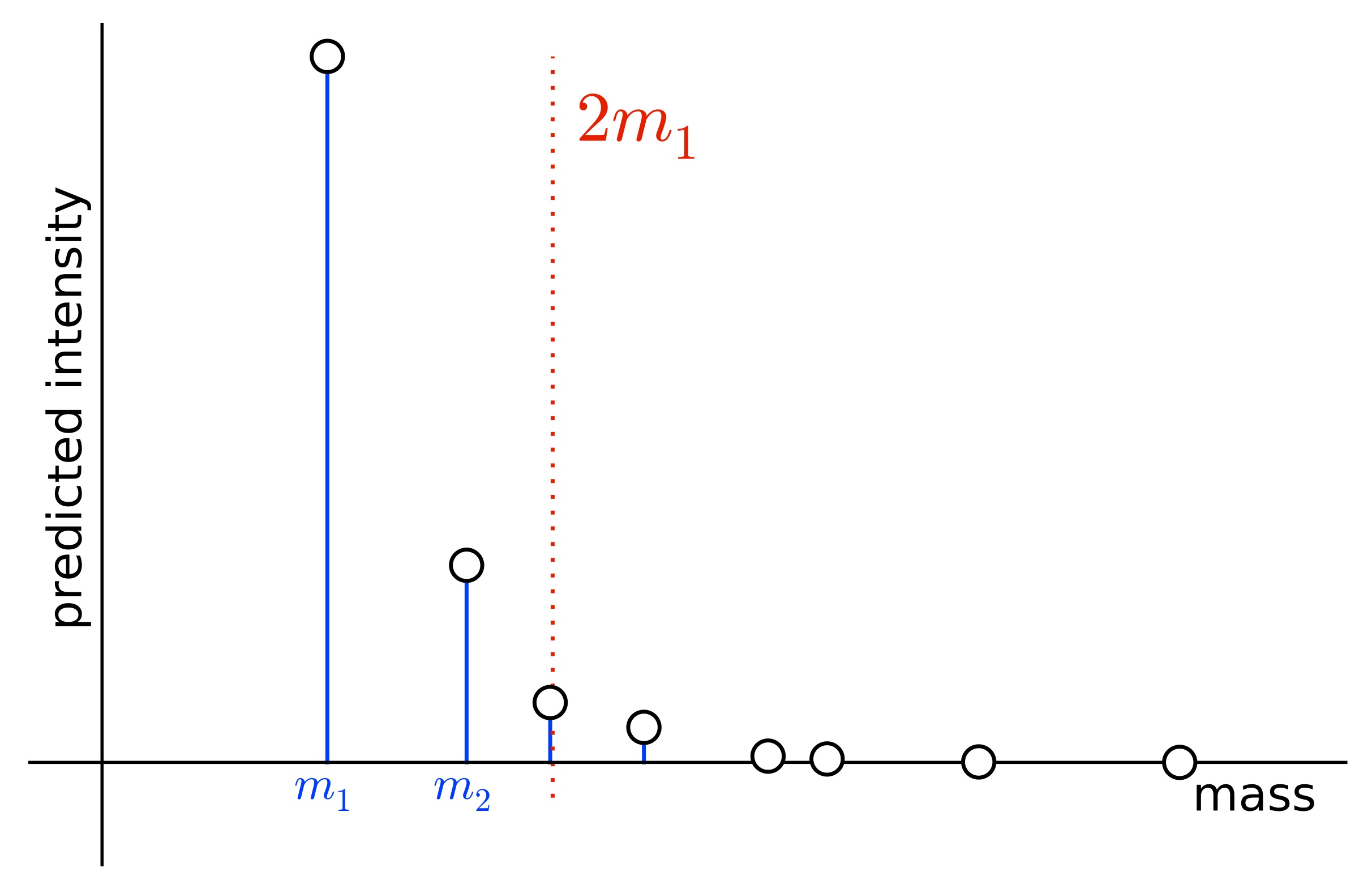
(B) Predictions

Figure 5. The left panel (A) is an example intensity plot, exhibiting the two detected masses under a transverse magnetic field of 5 tesla, 90% of the critical strength. (Figure adapted from [CTW⁺].) The right panel (B), shows the relative intensities obtained from the form factors computed in [DM, p. 741, Table 3]. The axes have the same labels as in the left panel. The dotted vertical line marks the onset of the incoherent continuum.

The two peaks give evidence of the existence of at least two particles in the system, which was one of Zamolodchikov’s core assumptions. And indeed, the ratio of the masses appears to approach the golden ratio—see Figure 6—as the critical value (about 5.5 T) is approached, just as Zamolodchikov predicted twenty years earlier.

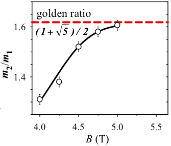
Figure 6. The ratio $m_{2}/m_{1}$ of the masses of the two lightest particles approaches the golden ratio as the transverse magnetic field approaches critical strength of 5.5 tesla. (Figure adapted from [CTW⁺].)

We can also compare the relative intensities of the first two mass peaks to the theoretical predictions exhibited in Figure 5B. Here again we see approximate agreement between the observations and theoretical predictions. The figure shows a threshold at $2m_{1}$, where a continuous spectrum is generated by the scattering of the lightest particle with itself. Particles with masses at or above this threshold will be very difficult to detect, as their energy signature is expected to consist of rather small peaks that overlap with the $2m_{1}$ continuum. Hence the fact that only two particles out of eight were observed is again consistent with the theoretical model.

9. Experimental evidence for ${{\mathsf{E}}_{8}}$ symmetry?

We can now finally address the question from the title of this paper, slightly rephrased: Did the experimenters detect ${{\mathsf{E}}_{8}}$? First we should say that they themselves do not claim to have done so. Rather, they claim to have found experimental evidence for the theory developed by Zamolodchikov, et al, and described above—which we shall call below simply Zamolodchikov’s theory—and that this in turn means giving evidence for ${{\mathsf{E}}_{8}}$ symmetry.

The argument for these claims goes as follows. The ${{\mathsf{E}}_{8}}$ ATFT is an integrable field theory describing the magnetically perturbed Ising model (2.1) and satisfying (Z1)–(Z4). In that situation, Zamolodchikov and Delfino-Mussardo made some numerical predictions regarding the relative masses of the particles and relative intensities of the scattering peaks. The experimental data show two peaks, but the second peak is only resolved at lower energies. The ratios of masses and intensities are certainly consistent with the theoretical predictions, although the ratios appear to be measured only rather roughly.

At this point, we want to address three objections to this line of argument that we heard when giving talks on the subject.

Objection #1: confirmatory experimental results are not evidence

We heard the following objection: experiments can never provide evidence for a scientific theory, they can only provide evidence against it. (This viewpoint is known as falsificationism.) This is of course preposterous. Science only progresses through the acceptance of theories that have survived enough good experimental tests, even if the words “enough” and “good” are open to subjective interpretations.

A less extreme version of this same objection is: confirmatory experimental results are automatically suspect in view of notorious historical examples of experimenter’s bias such as cold fusion and N-rays. This sort of objection is better addressed to the experimental physics community, which as a whole is certainly familiar with these specific examples and with the general issue of experimenter’s bias. As far as we know, no such criticisms have been raised concerning the methods described in [CTW⁺].

Objection #2: it still doesn’t seem like enough data

Recall that the experimental results can be summarized as a limited set of numbers which approximately agree with the theoretical predictions. Based on this, we have heard the following objection: if you start by looking at this small amount of data, how can you claim to have pinned down something as complex as ${{\mathsf{E}}_{8}}$? This question contains its own answer. One doesn’t analyze the results of the experiment by examining the data, divorced from all previous experience and theoretical framework. Instead, humanity already knows a lot about so-called critical point phenomena and there is a substantial theoretical model that is expected to describe the behavior of the magnet. The experiment described in [CTW⁺] was a test of the relevance and accuracy of Zamolodchikov’s theory, not an investigation of magnets beginning from no knowledge at all.

To put it another way, someone who approaches science from the viewpoint of this objector would necessarily reject many results from experimental physics that are based on similar sorts of indirect evidence. To give just one example of such a result, the reported observations of the top quark in [A⁺ 95a] and [A⁺ 95b] were not direct observations but rather confirmations of theoretical predictions made under the assumption that the top quark exists.

Objection #3: the numerical predictions don’t require ${{\mathsf{E}}_{8}}$

If you examine the papers [Z] by Zamolodchikov and [DM] by Delfino and Mussardo, you see that the numerical predictions are made without invoking ${{\mathsf{E}}_{8}}$. At this point, one might object that ${{\mathsf{E}}_{8}}$ is not strictly necessary for the theoretical model. But, as we explained in §5, the role of ${{\mathsf{E}}_{8}}$ in the theory is that by employing it, Zamolodchikov’s assumption (Z1) is turned into a deduction. That is, by including ${{\mathsf{E}}_{8}}$, we reduce the number of assumptions and achieve a more concise theoretical model. Moreover, the ${{\mathsf{E}}_{8}}$ version of the theory justifies the amazing numerological coincidences between Zamolodchikov’s calculations and the ${{\mathsf{E}}_{8}}$ root system.

Evidence for ${{\mathsf{E}}_{8}}$ symmetry?

Finally, we should address the distinction between “detecting ${{\mathsf{E}}_{8}}$” and “finding evidence for ${{\mathsf{E}}_{8}}$ symmetry”. While the former is pithier, we’re only talking about the latter here. The reason is that, as far as we know, there is no direct correspondence between ${{\mathsf{E}}_{8}}$ and any physical object. This is in contrast, for example, to the case of the gauge group $\operatorname{SU}(3)$ of the strong force in the Standard Model in particle physics. One can meaningfully identify basis vectors of the Lie algebra $\mathfrak{su}(3)$ with gluons, the mediators of the strong force, which have been observed in the laboratory. With this distinction in mind, our view is that the experiment cannot be said to have detected ${{\mathsf{E}}_{8}}$, but that it has provided evidence for Zamolodchikov’s theory and hence for ${{\mathsf{E}}_{8}}$ symmetry as claimed in [CTW⁺].

10. Summary

The experiment with the cobalt niobate magnet consisted of two phases. In the first phase, the experimenters verified that in the absence of an external magnetic field, the 1-dimensional quantum Ising model (2.1) accurately describes the spin dynamics, as predicted by theorists. In the second phase, the experimenters added an external magnetic field directed transverse to the spins’ preferred axis, and tuned this field close to the value required to reach the quantum critical regime. In that situation, Zamolodchikov, et al, had predicted the existence of 8 distinct types of particles in a field theory governed by the compact Lie algebra ${{\mathsf{E}}_{8}}$. The experimenters observed the two smallest particles and confirmed two numerical predictions: the ratio of the masses of the two smallest particles (predicted by Zamolodchikov) and the ratio of the intensities corresponding to those two particles (predicted by Delfino-Mussardo).

In this article, we have focused on the ${{\mathsf{E}}_{8}}$ side of the story because ${{\mathsf{E}}_{8}}$ is a mathematical celebrity. But there is a serious scientific reason to be interested in the experiment apart from ${{\mathsf{E}}_{8}}$: it is the first experimental test of the perturbed conformal field theory constructed by Zamolodchikov around 1990. Also, it is the first laboratory realization of the critical state of the quantum 1-dimensional Ising model in such a way that it can be manipulated—the experimenters can continuously vary the transverse field strength $g_{x}$ in (2.1) across a wide range while preserving the 1-dimensional character—and the results observed directly. Since the Ising model is the fundamental model for quantum phase transitions, the opportunity to probe experimentally its very rich physics represents a breakthrough.

References

- [A+ 95a] S. Abachi et al., Search for high mass top quark production in collisions at TeV, Phys. Rev. Lett. 74 (1995), no. 13, 2422–2426.
- [A+ 95b] F. Abe et al., Observation of top quark production in collisions with the Collider Detector at Fermilab, Phys. Rev. Lett. 74 (1995), no. 14, 2626–2631.
- [BLM] S. Berman, Y.S. Lee, and R.V. Moody, The spectrum of a Coxeter transformation, affine Coxeter transformations, and the defect map, J. Algebra 121 (1989), no. 2, 339–357.
- [Bo] N. Bourbaki, Lie groups and Lie algebras: Chapters 4–6, Springer-Verlag, Berlin, 2002.
- [BPZ] A.A. Belavin, A.M. Polyakov, and A.B. Zamolodchikov, Infinite conformal symmetry in two-dimensional quantum field theory, Nuclear Phys. B 241 (1984), 333–380.
- [Br] H.W. Braden, A note on affine Toda couplings, J. Phys. A 25 (1992), L15–L20.
- [BRA] D. Bitko, T.F. Rosenbaum, and G. Aeppli, Quantum critical behavior for a model magnet, Phys. Rev. Lett. 77 (1996), 940–943.
- [Ca] R.W. Carter, Simple groups of Lie type, Wiley, 1989.
- [Cor] E. Corrigan, Recent developments in affine Toda quantum field theory, Particles and fields (G.W. Semenoff and L. Vinet, eds.), Springer, 1999, also available at arXiv:hep-th/9412213, pp. 1–34.
- [Cox] H.S.M. Coxeter, Regular complex polytopes, Cambridge University Press, 1991.
- [CT] S.T. Carr and A.M. Tsvelik, Spectrum and correlation functions of a quasi-one-dimensional quantum Ising model, Physical Rev. Letters 90 (2003), no. 17, 177206.
- [CTW+] R. Coldea, D.A. Tennant, E.M. Wheeler, E. Wawrzynska, D. Prabhakaran, M. Telling, K. Habicht, P. Smibidl, and K. Kiefer, Quantum criticality in an Ising chain: experimental evidence for emergent symmetry, Science 327 (2010), 177–180.
- [DFMS] P. Di Francesco, P. Mathieu, and D. Sénéchal, Conformal field theory, Graduate Texts in Contemporary Physics, Springer-Verlag, New York, 1997.
- [DG10] J. Distler and S. Garibaldi, There is no “Theory of Everything” inside , Comm. Math. Phys. 298 (2010), 419–436.
- [DM] G. Delfino and G. Mussardo, The spin-spin correlation function in the two-dimensional Ising model in a magnetic field at , Nuclear Phys. B (1995), 724–758.
- [Do] P. Dorey, Root systems and purely elastic -matrices, Nuclear Phys. B 358 (1991), no. 3, 654–676.
- [EY] T. Eguchi and S.-K. Yang, Deformations of conformal field theories and soliton equations, Phys. Lett. B 224 (1989), no. 4, 373–378.
- [FLO] A. Fring, H.C. Liao, and D.I. Olive, The mass spectrum and coupling in affine Toda theories, Phys. Lett. B 266 (1991), 82–86.
- [Fo] G. B. Folland, Speaking with the natives: reflections on mathematical communication, Notices Amer. Math. Soc. 57 (2010), no. 9, 1121–1124.
- [FQS] D. Friedan, Z. Qiu, and S. Shenker, Conformal invariance, unitarity, and critical exponents in two dimensions, Phys. Rev. Lett. 52 (1984), no. 18, 1575–1578.
- [Fr] M.D. Freeman, On the mass spectrum of affine Toda field theory, Phys. Lett. B 261 (1991), no. 1-2, 57–61.
- [FZ] V.A. Fateev and A.B. Zamolodchikov, Conformal field theory and purely elastic -matrices, Internat. J. Modern Phys. A 5 (1990), no. 6, 1025–1048.
- [GHMR] D.J. Gross, J.A. Harvey, E. Martinec, and R. Rohm, Heterotic string, Physical Review Letters 54 (1985), no. 6, 502–505.
- [GKO] P. Goddard, A. Kent, and D. Olive, Virasoro algebras and coset space models, Phys. Letters B 152 (1985), no. 1–2, 88–92.
- [GaS] S. Garibaldi and N. Semenov, Degree 5 invariant of , Int. Math. Res. Not. IMRN (2010), no. 19, 3746–3762.
- [He] M. Henkel, Conformal invariance and critical phenomena, Texts and Monographs in Physics, Springer-Verlag, Berlin, 1999.
- [HeS] M. Henkel and H. Saleur, The two-dimensional Ising model in a magnetic field: a numerical check of Zamolodchikov’s conjecture, J. Phys. A 22 (1989), 513–518.
- [HoM] T.J. Hollowood and P. Mansfield, Rational conformal field theories at, and away from, criticality as Toda field theories, Phys. Lett. B 226 (1989), no. 1–2, 73–79.
- [I] E. Ising, Beitrag zur Theorie des Ferromagnetismus, Z. Phys. 31 (1925), 253–258.
- [J 71] N. Jacobson, Exceptional Lie algebras, Lecture notes in pure and applied mathematics, vol. 1, Marcel-Dekker, New York, 1971.
- [J 79] by same author, Lie algebras, Dover, 1979.
- [K 59] B. Kostant, The principal three-dimensional subgroup and the Betti numbers of a complex simple Lie group, Amer. J. Math. 81 (1959), 973–1032.
- [K 85] by same author, The McKay correspondence, the Coxeter element and representation theory, Astérisque (1985), no. Numero Hors Serie, 209–255, The mathematical heritage of Élie Cartan (Lyon, 1984).
- [K 10] by same author, Experimental evidence for the occurrence of in nature and the radii of the Gosset circles, Selecta Math. (NS) 16 (2010), no. 3, 419–438.
- [L] A. Garrett Lisi, An exceptionally simple theory of everything, arXiv:0711.0770 [hep-th], 2007.
- [MS] N. Marcus and J.H. Schwarz, Three-dimensional supergravity theories, Nuclear Phys. B 228 (1983), no. 1, 145–162.
- [Mu] G. Mussardo, Statistical field theory, Oxford Graduate Texts, Oxford University Press, Oxford, 2010.
- [MW 73] B.M. McCoy and T.T. Wu, The two-dimensional Ising model, Harvard University Press, 1973.
- [MW 78] by same author, Two-dimensional Ising field theory in a magnetic field: breakup of the cut in the two-point function, Phys. Rev. D 18 (1978), no. 4, 1259–1267.
- [O] L. Onsager, Crystal statistics. I. A two-dimensional model with an order-disorder transition, Phys. Rev. (2) 65 (1944), 117–149.
- [P] A.M. Polyakov, Conformal symmetry of critical fluctuations, JETP Lett. 12 (1970), 381.
- [Sa] S. Sachdev, Quantum phase transitions, Cambridge University Press, Cambridge, 1999.
- [Se 79] J-P. Serre, Local fields, Graduate Texts in Mathematics, vol. 67, Springer, New York-Berlin, 1979.
- [Se 02] by same author, Galois cohomology, Springer-Verlag, 2002, originally published as Cohomologie galoisienne (1965).
- [St] J. Stembridge, Coxeter planes, http://www.math.lsa.umich.edu/~jrs/coxplane.html.
- [SZ] I.R. Sagdeev and A.B. Zamolodchikov, Numerical check of the exact mass spectrum of the scaling limit of Ising model with magnetic field, Modern Physics Letters B 3 (1989), no. 18, 1375–1381.
- [TFV] M.J. Tejwani, O. Ferreira, and O.E. Vilches, Possible Ising transition in a 4He monolayer adsorbed on Kr-plated graphite, Phys. Rev. Letters 44 (1980), no. 3, 152–155.
- [V] D. Vogan, The character table for , Notices of the AMS 54 (2007), no. 9, 1022–1034.
- [Z] A.B. Zamolodchikov, Integrals of motion and -matrix of the (scaled) Ising model with magnetic field, Int. J. Modern Physics 4 (1989), no. 16, 4235–4248.