The method of unitary clothing transformations in the theory of nucleon–nucleon scattering

Abstract

The clothing procedure, put forward in quantum field theory (QFT) by Greenberg and Schweber, is applied for the description of nucleon–nucleon ($N-N$) scattering. We consider pseudoscalar ($\pi$ and $\eta$), vector ($\rho$ and $\omega$) and scalar ($\delta$ and $\sigma$) meson fields interacting with $1/2$ spin ($N$ and $\bar{N}$) fermion ones via the Yukawa–type couplings to introduce trial interactions between ”bare” particles. The subsequent unitary clothing transformations (UCTs) are found to express the total Hamiltonian through new interaction operators that refer to particles with physical (observable) properties, the so–called clothed particles. In this work, we are focused upon the Hermitian and energy–independent operators for the clothed nucleons, being built up in the second order in the coupling constants. The corresponding analytic expressions in momentum space are compared with the separate meson contributions to the one–boson–exchange potentials in the meson theory of nuclear forces. In order to evaluate the $T$ matrix of the $N-N$ scattering we have used an equivalence theorem that enables us to operate in the clothed particle representation (CPR) instead of the bare particle representation (BPR) with its large amount of virtual processes. We have derived the Lippmann–Schwinger type equation for the CPR elements of the $T-$ matrix for a given collision energy in the two–nucleon sector of the Hilbert space $\mathcal{H}$ of hadronic states.

1 Introductory remarks and some recollections

We know that there are a number of high precision, boson-exchange models of the two nucleon force $V_{NN}$, such as Paris Lacom80 , Bonn MachHolElst87 , Nijmegen Stocks94 , Argonne WirStocksSchia95 , CD Bonn Mach01 potentials and a modern family of covariant one-boson-exchange (OBE) ones GrossStad08 .Note also successful treatments based on chiral effective field theory OrdoRayKolck94 ,EpelGloeMeiss00 , for a review see Epel05 .

In this paper, we would like to draw attention to the first application of unitary clothing transformations (UCTs) SheShi01 ; KorCanShe07 in describing the nucleon–nucleon scattering. Recall that such transformations $W$, being aimed at the inclusion of the so–called cloud or persistent effects, make it possible the transition from the bare–particle representation (BPR) to the clothed–particle representation (CPR) in the Hilbert space $\mathcal{H}$ of meson–nucleon states. In this way, a large amount of virtual processes induced with the meson absorption/emission, the $N\overline{N}-$pair annihilation/production and other cloud effects can be accumulated in the creation (destruction) operators $\alpha_{c}$ for the ”clothed” (physical) mesons and nucleons. Such a bootstrap reflects the most significant distinction between the concepts of clothed and bare particles.

In the course of the clothing procedure all the generators of the Poincaré group get one and the same sparse structure on $\mathcal{H}$ SheShi01 . Here we will focus upon one of them, viz., the total Hamiltonian

$$H=H_{F}(\alpha)+H_{I}(\alpha)\equiv H(\alpha)$$ (1)

with

$$H_{I}(\alpha)=V(\alpha)+\mbox{mass and vertex counterterms},$$ (2)

where free part $H_{F}(\alpha)\sim\alpha^{{\dagger}}\alpha$ belongs to the class [1.1], if one uses the terminology adopted in SheShi01 , and interaction $V(\alpha)$ is a function of creation (destruction) operators $\alpha^{{\dagger}}(\alpha)$ in the BPR, i.e., referred to bare particles with physical masses KorCanShe07 , where they have been introduced via the mass–changing Bogoliubov–type UTs. To be more definite, let us consider fermions (nucleons and antinucleons) and bosons ($\pi-$, $\eta-$, $\rho-$, $\omega$-mesons, etc.) interacting via the Yukawa-type couplings for scalar (s), pseudoscalar (ps) and vector (v) mesons. Then, as seen from Appendix A, $V(\alpha)=V_{s}+V_{ps}+V_{\rm{v}}$ with

$$V_{s}=g_{s}\int d\vec{x}\,\bar{\psi}(\vec{x})\psi(\vec{x})\varphi_{s}(\vec{x})$$ (3)

$$V_{ps}=ig_{ps}\int d\vec{x}\,\bar{\psi}(\vec{x})\gamma_{5}\psi(\vec{x})\varphi_{ps}(\vec{x})$$ (4)

$$V_{\rm{v}}=\int d\vec{x}\,\left\{g_{\rm{v}}\bar{\psi}(\vec{x})\gamma_{\mu}\psi(\vec{x})\varphi_{\rm{v}}^{\mu}(\vec{x})\phantom{\frac{f_{\rm{v}}}{4m}}\right.\\ \left.+\frac{f_{\rm{v}}}{4m}\bar{\psi}(\vec{x})\sigma_{\mu\nu}\psi(\vec{x})\varphi_{\rm{v}}^{\mu\nu}(\vec{x})\right\}\\ +\int d\vec{x}\,\left\{\frac{g_{\rm{v}}^{2}}{2m_{\rm{v}}^{2}}\bar{\psi}(\vec{x})\gamma_{0}\psi(\vec{x})\bar{\psi}(\vec{x})\gamma_{0}\psi(\vec{x})\right.\\ \left.+\frac{f_{\rm{v}}^{2}}{4m^{2}}\bar{\psi}(\vec{x})\sigma_{0i}\psi(\vec{x})\bar{\psi}(\vec{x})\sigma_{0i}\psi(\vec{x})\right\},$$ (5)

where $\varphi_{\rm{v}}^{\mu\nu}(\vec{x})=\partial^{\mu}\varphi_{\rm{v}}^{\nu}(\vec{x})-\partial^{\nu}\varphi_{\rm{v}}^{\mu}(\vec{x})$ the tensor of the vector field included. The mass (vertex) counterterms are given by Eqs. (32)–(33) of Ref. KorCanShe07 (the difference $V_{0}(\alpha)$ - $V(\alpha)$ where a primary interaction $V_{0}(\alpha)$ is derived from $V(\alpha)$ replacing the ”physical” coupling constants by ”bare” ones).

The corresponding set $\alpha$ involves operators $a^{{\dagger}}(a)$ for the bosons, $b^{{\dagger}}(b)$ for the nucleons and $d^{{\dagger}}(d)$ for the antinucleons. Following a common practice, they appear in the standard Fourier expansions of the boson fields $\varphi_{b}$ and the fermion field $\psi$, though for our purposes the use of such a representation is not compulsory (see, e.g., Chapter 3 of the monograph WeinbergBook1995 ). In any case we have the free pion and fermion parts

$$H_{F}(\alpha)=\int d\vec{k}\,\omega_{\vec{k}}a^{\dagger}(\vec{k})a(\vec{k})\\ +\int d\vec{p}\,E_{\vec{p}}\sum\limits_{\mu}\left[b^{\dagger}(\vec{p},\mu)b(\vec{p},\mu)+d^{\dagger}(\vec{p},\mu)d(\vec{p},\mu)\right]$$ (6)

and the primary trilinear interaction

$$V(\alpha)\sim ab^{{\dagger}}b+ab^{{\dagger}}d^{{\dagger}}+adb+add^{{\dagger}}+H.c.$$ (7)

with the three-legs vertices. Here $\omega_{\vec{k}}=\sqrt{m^{2}_{b}+\vec{k}^{2}}\,\,$ ($E_{\vec{p}}=\sqrt{m^{2}+\vec{p}^{2}}$) represents the pion (nucleon) energy with physical mass $m_{b}(m)$ while $\mu$ denotes the fermion polarization index. It may be the particle spin projection onto the quantization axis ( the particle momentum ) for the so–called canonical ( helicity–state ) basis ( see, e.g., Chapter 4 of Ref. Gas66 ).

In the context, we have tried to draw parallels with that field–theoretic background which has been employed in boson–exchange models. First of all, we imply the approach by the Bonn group MachHolElst87 ; Mach01 , where, following the idea by Schütte Schutte , the authors started from the total Hamiltonian (in our notations),

$$H=H_{F}(\alpha)+V(\alpha)$$ (8)

with the boson-nucleon interaction

$$V(\alpha)\sim ab^{{\dagger}}b+H.c.$$ (9)

For brevity, the contributions from other mesons are omitted.

Unlike Eq.(7) the antinucleonic degrees of freedom were disregarded in Ref. MachHolElst87 . There (see also Gas66 ) the transition matrix $T(z)$ (in the two–nucleon space) was considered in the framework of the three-dimensional perturbation theory when handling the integral equation,

$$T_{NN}(z)=V_{NN}(z)+V_{NN}(z)(z-H_{N})^{-1}T_{NN}(z),$$ (10)

where the energy–dependent ”quasipotential” $V_{NN}(z)$ approximates a sum of all relevant non-iterative diagrams, $H_{N}$ the nucleon contribution to $H_{F}$. Such a potential has ”the unpleasant feature of being energy–dependent. This complicates applications to nuclear structure physics considerably” (quoted from p.40 in MachHolElst87 ). Therefore, further simplifications are welcome (see, e.g., Refs. MachHolElst87 , Mach01 ).

Along with our derivation of a Lippmann–Schwinger (LS) equation for the T matrix of the $N-N$ scattering, we will demonstrate its solutions to be compared with those by the Bonn group.

2 Analytic expressions for the quasipotentials in momentum space

As shown in SheShi01 , after eliminating the so-called bad terms from $V(\alpha)$ the primary Hamiltonian $H(\alpha)$ can be represented in the form,

$$H(\alpha)=K_{F}(\alpha_{c})+K_{I}(\alpha_{c})\equiv K(\alpha_{c})$$ (11)

The free part of the new decomposition is determined by

$$K_{F}(\alpha_{c})=\int d\vec{k}\,\omega_{\vec{k}}a_{c}^{\dagger}(\vec{k})a_{c}(\vec{k})\\ +\int d\vec{p}\,E_{\vec{p}}\sum\limits_{\mu}\left[b_{c}^{\dagger}(\vec{p},\mu)b_{c}(\vec{p},\mu)+d_{c}^{\dagger}(\vec{p},\mu)d_{c}(\vec{p},\mu)\right]$$ (12)

while $K_{I}$ contains only interactions responsible for physical processes, these quasipotentials between the clothed particles, e.g.,

$$K_{I}^{(2)}(\alpha_{c})=K(NN\to NN)+K(\bar{N}\bar{N}\to\bar{N}\bar{N})\\ +K(N\bar{N}\to N\bar{N})+K(bN\to bN)+K(b\bar{N}\to b\bar{N})\\ +K(bb^{\prime}\to N\bar{N})+K(N\bar{N}\to bb^{\prime})$$ (13)

A key point of the clothing procedure developed in SheShi01 is to fulfill the following requirements:

i) The physical vacuum (the $H$ lowest eigenstate) must coincide with a new no–particle state $\Omega$, i.e., the state that obeys the equations

$$a_{c}(\vec{k})\left|\Omega\right\rangle=b_{c}(\vec{p},\mu)\left|\Omega\right\rangle=d_{c}(\vec{p},\mu)\left|\Omega\right\rangle=0,\,\,\,\forall\,\,{\vec{k},\,\vec{p},\,\mu}$$ (14)

$$\left\langle\Omega|\Omega\right\rangle=1.$$

ii) New one-clothed-particle states $|\vec{k}\rangle_{c}\equiv a_{c}^{{\dagger}}(\vec{k})\Omega$ etc. are the eigenvectors both of $K_{F}$ and $K$,

$$K(\alpha_{c})|\vec{k}\rangle_{c}=K_{F}(\alpha_{c})|\vec{k}\rangle_{c}=\omega_{k}|\vec{k}\rangle_{c}$$ (15)

$$K_{I}(\alpha_{c})|\vec{k}\rangle_{c}=0$$ (16)

iii) The spectrum of indices that enumerate the new operators must be the same as that for the bare ones .

iv) The new operators $\alpha_{c}$ satisfy the same commutation rules as do their bare counterparts $\alpha$, since the both sets are connected to each other via the similarity transformation

$$\alpha_{c}=W^{{\dagger}}\alpha W,$$ (17)

with a unitary operator $W$ to be obtained as in SheShi01 .

It is important to realize that operator $K(\alpha_{c})$ is the same Hamiltonian $H(\alpha)$. Accordingly [10,11] the $N$–$N$ interaction operator in the CPR has the following structure:

$$K(NN\rightarrow NN)=\sum\limits_{b}K_{b}(NN\rightarrow NN),$$

$$K_{b}(NN\rightarrow NN)=\int\sum\limits_{\mu}d\vec{p}^{\prime}_{1}\,d\vec{p}^{\prime}_{2}\,d\vec{p}_{1}\,d\vec{p}_{2}\\ \times V_{b}(1^{\prime},2^{\prime};1,2)b_{c}^{\dagger}(1^{\prime})b_{c}^{\dagger}(2^{\prime})b_{c}(1)b_{c}(2),$$ (18)

where the symbol $\sum\limits_{\mu}$ denotes the summation over the nucleon spin projections, $1=\{\vec{p}_{1},\mu_{1}\}$, etc.

For our evaluations of the c–number matrices $V_{b}$ we have employed some experience from Refs. SheShi01 ; KorCanShe07 to get in the second order in the coupling constants (see Appendix A)

$$V_{b}(1^{\prime},2^{\prime};1,2)=\frac{1}{(2\pi)^{3}}\frac{m^{2}}{\sqrt{E_{\vec{p}^{\prime}_{1}}E_{\vec{p}^{\prime}_{2}}E_{\vec{p}_{1}}E_{\vec{p}_{2}}}}\\ \times\delta\left(\vec{p}^{\prime}_{1}+\vec{p}^{\prime}_{2}-\vec{p}_{1}-\vec{p}_{2}\right)v_{b}(1^{\prime},2^{\prime};1,2),$$ (19)

$$v_{s}(1^{\prime},2^{\prime};1,2)\\ =-\frac{g_{s}^{2}}{2}\bar{u}(\vec{p}^{\prime}_{1})u(\vec{p}_{1})\frac{1}{(p_{1}-p^{\prime}_{1})^{2}-m_{s}^{2}}\bar{u}(\vec{p}^{\prime}_{2})u(\vec{p}_{2}),$$ (20)

$$v_{ps}(1^{\prime},2^{\prime};1,2)\\ =\frac{g_{ps}^{2}}{2}\bar{u}(\vec{p}^{\prime}_{1})\gamma_{5}u(\vec{p}_{1})\frac{1}{(p_{1}-p^{\prime}_{1})^{2}-m_{ps}^{2}}\bar{u}(\vec{p}^{\prime}_{2})\gamma_{5}u(\vec{p}_{2}),$$ (21)

$$v_{\rm{v}}(1^{\prime},2^{\prime};1,2)=\frac{1}{2}\frac{1}{(p^{\prime}_{1}-p_{1})^{2}-m_{\rm{v}}^{2}}\\ \times\left[\bar{u}(\vec{p}^{\prime}_{1})\left\{(g_{\rm{v}}+f_{\rm{v}})\gamma_{\nu}-\frac{f_{\rm{v}}}{2m}(p^{\prime}_{1}+p_{1})_{\nu}\right\}u(\vec{p}_{1})\right.\\ \times\bar{u}(\vec{p}^{\prime}_{2})\left\{(g_{\rm{v}}+f_{\rm{v}})\gamma^{\nu}-\frac{f_{\rm{v}}}{2m}(p^{\prime}_{2}+p_{2})^{\nu}\right\}u(\vec{p}_{2})\\ -\bar{u}(\vec{p}^{\prime}_{1})\left\{(g_{\rm{v}}+f_{\rm{v}})\gamma_{\nu}-\frac{f_{\rm{v}}}{2m}(p^{\prime}_{1}+p_{1})_{\nu}\right\}u(\vec{p}_{1})\\ \times\bar{u}(\vec{p}^{\prime}_{2})\frac{f_{\rm{v}}}{2m}\left\{(\hat{p}_{1}^{\prime}+\hat{p}_{2}^{\prime}-\hat{p}_{1}-\hat{p}_{2})\gamma^{\nu}\right.\\ \left.\phantom{\frac{f_{\rm{v}}}{2m}}\left.-(p^{\prime}_{1}+p^{\prime}_{2}-p_{1}-p_{2})^{\nu}\right\}u(\vec{p}_{2})\right],$$ (22)

where $m_{b}$ the mass of the clothed boson (its physical value) and $\hat{q}=q_{\mu}\gamma^{\mu}$. In the framework of the isospin formalism one needs to add the factor $\vec{\tau}(1)\vec{\tau}(2)$ in the corresponding expressions.

One should stress that in the course of our derivations the Feynman propagator

$$\left[(p_{1}-p_{1}^{\prime})^{2}-m^{2}_{b}\right]^{-1}$$

arises from adding the noncovariant propagators

$$\left[2\omega_{\vec{k}}\left(E_{\vec{p}_{1}}-E_{\vec{p}^{\prime}_{1}}-\omega_{\vec{k}}\right)\right]^{-1}$$

and

$$\left[2\omega_{\vec{k}}\left(E_{\vec{p}^{\prime}_{1}}-E_{\vec{p}_{1}}-\omega_{\vec{k}}\right)\right]^{-1}.$$

Such a feature of the UCTs method allows us to use the graphic language of the old-fashioned perturbation theory (OFPT) (see, e.g., Chapter 13 in Schweber’s book SchweberBook ) when addressing the graphs in Fig.1.

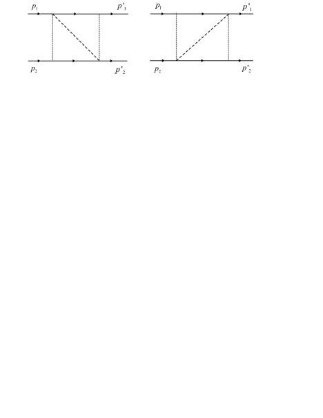
Figure 1: The typical OFPT diagrams with the intermediate boson (dashed lines) on its mass shell.

As noted in KorCanShe07 the graphs within our approach should not be interpreted as the two time-ordered Feynmam diagrams. Indeed, all events in the S picture used here are related to the same instant $t=0$. Being aware of this, the line directions in Fig.1 are given with the sole scope to discriminate between nucleons and antinucleons. The latter will inevitably appear in higher orders in coupling constants and for other physical processes (e.g., the $\pi N$ scattering) as it has been demonstrated in Ref. KorCanShe07 .

Further, for each boson included the corresponding relativistic and properly symmetrized $N-N$ interaction, the kernel of integral equations for the $N-N$ bound and scattering states, is determined by

$$\left\langle b_{c}^{\dagger}(\vec{p}^{\prime}_{1})b_{c}^{\dagger}(\vec{p}^{\prime}_{2})\Omega\right|K_{b}(NN\rightarrow NN)\left|b_{c}^{\dagger}(\vec{p}_{1})b_{c}^{\dagger}(\vec{p}_{2})\Omega\right\rangle\\ =V_{b}^{dir}(1^{\prime},2^{\prime};1,2)-V_{b}^{exc}(1^{\prime},2^{\prime};1,2)$$ (23)

where we have separated the so–called direct

$$V_{b}^{dir}(1^{\prime},2^{\prime};1,2)=-V_{b}(1^{\prime},2^{\prime};1,2)-V_{b}(2^{\prime},1^{\prime};2,1)$$ (24)

and exchange

$$V_{b}^{exc}(1^{\prime},2^{\prime};1,2)=V_{b}^{dir}(2^{\prime},1^{\prime};1,2)$$ (25)

terms. For example, the one–pion–exchange contribution can be divided into the two parts:

$$V_{\pi}^{dir}(1^{\prime},2^{\prime};1,2)=-\frac{g_{\pi}^{2}}{(2\pi)^{3}}\frac{m^{2}}{\sqrt{E_{\vec{p}^{\prime}_{1}}E_{\vec{p}^{\prime}_{2}}E_{\vec{p}_{1}}E_{\vec{p}_{2}}}}\\ \times\delta\left(\vec{p}^{\prime}_{1}+\vec{p}^{\prime}_{2}-\vec{p}_{1}-\vec{p}_{2}\right)\bar{u}(\vec{p}^{\prime}_{1})\gamma_{5}u(\vec{p}_{1})\bar{u}(\vec{p}^{\prime}_{2})\gamma_{5}u(\vec{p}_{2})\\ \times\frac{1}{2}\left\{\frac{1}{(p_{1}-p^{\prime}_{1})^{2}-m_{\pi}^{2}}+\frac{1}{(p_{2}-p^{\prime}_{2})^{2}-m_{\pi}^{2}}\right\}$$ (26)

and

$$V_{\pi}^{exc}(1^{\prime},2^{\prime};1,2)=-\frac{g_{\pi}^{2}}{(2\pi)^{3}}\frac{m^{2}}{\sqrt{E_{\vec{p}^{\prime}_{1}}E_{\vec{p}^{\prime}_{2}}E_{\vec{p}_{1}}E_{\vec{p}_{2}}}}\\ \times\delta\left(\vec{p}^{\prime}_{1}+\vec{p}^{\prime}_{2}-\vec{p}_{1}-\vec{p}_{2}\right)\bar{u}(\vec{p}^{\prime}_{1})\gamma_{5}u(\vec{p}_{2})\bar{u}(\vec{p}^{\prime}_{2})\gamma_{5}u(\vec{p}_{1})\\ \times\frac{1}{2}\left\{\frac{1}{(p_{2}-p^{\prime}_{1})^{2}-m_{\pi}^{2}}+\frac{1}{(p_{1}-p^{\prime}_{2})^{2}-m_{\pi}^{2}}\right\}$$ (27)

to be depicted in Fig. 2, where the dashed lines correspond to the following Feynman–like ”propagators”:

$$\frac{1}{2}\left\{\frac{1}{(p_{1}-p^{\prime}_{1})^{2}-m_{\pi}^{2}}+\frac{1}{(p_{2}-p^{\prime}_{2})^{2}-m_{\pi}^{2}}\right\}$$

on the left panel and

$$\frac{1}{2}\left\{\frac{1}{(p_{2}-p^{\prime}_{1})^{2}-m_{\pi}^{2}}+\frac{1}{(p_{1}-p^{\prime}_{2})^{2}-m_{\pi}^{2}}\right\}$$

on the right panel. Other distinctive features of the result (23) have been discussed in SheShi01 ; KorCanShe07 . Note also that expressions (26)–(27) determine the one–pion–exchange part of one–boson–exchange interaction derived via the Okubo transformation method in KOSHE93 ( cf. FudaZhang95 ; KorCanShe07 ) taking into account the pion and heavier–meson exchanges.

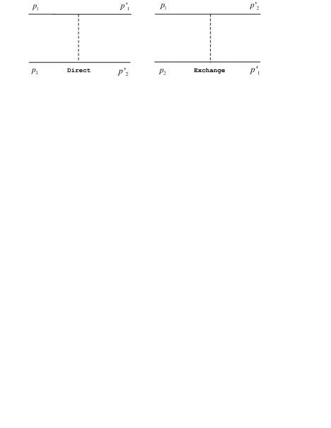
Figure 2: The Feynman–like diagrams for the direct and exchange contributions in the r.h.s. of Eq.(23).

3 The field–theoretic description of the elastic $N$–$N$ scattering

3.1 The $T$–matrix in the CPR

Usually in nonrelativistic quantum mechanics (NQM) the LS equation for the T operator

$$T(E+i0)=V_{NN}+V_{NN}(E+i0-h_{0})^{-1}T(E+i0)$$ (28)

with a given kernel $V_{NN}$ is a starting point in evaluating the $N$-$N$ phase shifts. All operators in Eq. (28) (including the sum $h_{0}$ of the nucleon kinetic energies) act onto the subspace of two–nucleon states, and remain confined in this subspace (the particle number is conserved within nonrelativistic approach). The matrix elements $\langle N^{\prime}N^{\prime}|T(E+i0)|NN\rangle,$ form the corresponding $T-$ matrix and, at the collision energy

$$E=E_{1}+E_{2}=E_{1}^{{}^{\prime}}+E_{2}^{{}^{\prime}},$$

the on–energy–shell elements can be expressed through the phase shifts and mixing parameters (see below).

In relativistic QFT the situation is completely different. Though one can formally introduce a field operator $T$ that meets the equation

$$T(E+i0)=H_{I}+H_{I}(E+i0-H_{F})^{-1}T(E+i0)$$ (29)

the field interaction $H_{I}$, as a rule, does not conserve the particle number, being the spring of particle creation and destruction. The feature makes the problem of finding the $N$–$N$ scattering matrix much more complicated than in the framework of nonrelativistic approach, since now the $T$ matrix enters an infinite set of coupled integral equations.

Such a general field–theoretic consideration can be simplified with the help of an equivalence theorem ShebekoFB17 ; SheISHEPP02 according to which the $S$ matrix elements in the Dirac (D) picture, viz.,

$$S_{fi}\equiv\langle\alpha^{{\dagger}}...\Omega_{0}|S(\alpha)|\alpha^{{\dagger}}...\Omega_{0}\rangle$$ (30)

are equal to the corresponding elements

$$S_{fi}^{c}\equiv\langle\alpha_{c}^{{\dagger}}...\Omega|S(\alpha_{c})|\alpha_{c}^{{\dagger}}...\Omega\rangle$$ (31)

of the $S$ matrix in the CPR. We say ”corresponding” keeping in mind the requirement $iii$) of Sec. 2. The $S$ operators in Eqs. (30)–(31) are determined by the time evolution from the distant past to the distant future, respectively, for the two decompositions

$$H=H(\alpha)=H_{F}+H_{I}$$

and

$$H=K(\alpha_{c})=K_{F}+K_{I}$$

Note that the equality $S_{fi}=S_{fi}^{c}$ in question becomes possible owing to certain isomorphism between the $\alpha_{c}$ algebra and the $\alpha$ algebra once the UCTs $W_{D}(t)=\exp(iK_{F}t)W\exp(-iK_{F}t)$ obey the condition

$$W_{D}(\pm\infty)=1$$ (32)

The $T$ operator in the CPR satisfies the equation

$$T_{cloth}(E+i0)=K_{I}\\ +K_{I}(E+i0-K_{F})^{-1}T_{cloth}(E+i0)$$ (33)

and the matrix

$$T_{fi}\equiv\langle f;b|T(E+i0)|i;b\rangle\\ =\langle f;c|T_{cloth}(E+i0)|i;c\rangle\equiv T_{fi}^{c},$$ (34)

where $|;b\rangle$ ( $|;c\rangle$ ) are the $H_{F}$ ( $K_{F}$ ) eigenvectors, may be evaluated relying upon properties of the new interaction $K_{I}(\alpha_{c})$. The latter has nonzero matrix elements only between the clothed–particle (physical) states. Such a restriction helps us to facilitate the further consideration compared to the BPR with its large amount of virtual transitions (cf., our discussion in Sect.1 ).

If in Eq.(33) we approximate $K_{I}$ by $K_{I}^{(2)}$ (see Eq.(13)), then initial task of evaluating the BPR matrix elements $\langle N^{\prime}N^{\prime}|T(E+i0)|NN\rangle$ can be reduced to solving the equation

$$\langle 1^{\prime},2^{\prime}|T_{NN}(E)|1,2\rangle=\langle 1^{\prime},2^{\prime}|K_{NN}|1,2\rangle\\ +\langle 1^{\prime},2^{\prime}|K_{NN}(E+i0-K_{F})^{-1}T_{NN}(E)|1,2\rangle$$ (35)

with $K_{NN}=K(NN\rightarrow NN)$.

Actually, let us employ the relation,

$$G_{F}(z)T_{cloth}(z)=G(z)K_{I}$$ (36)

with the two resolvents

$$G_{F}(z)=(z-K_{F})^{-1}\,\,\,\,\,\,G(z)=(z-K)^{-1}$$

In its turn, Eq.(36) can be rewritten as

$$iG_{F}(z)T_{cloth}(z)=\int\limits_{0}^{\infty}d\tau e^{i(z-K)\tau}K_{I}$$ (37)

To the approximation in question, where

$$K\simeq K_{F}+K_{I}^{(2)}\equiv K_{2}+K_{4}$$ (38)

with

$$K_{2}=K_{2}(ferm)+K_{2}(mes),$$

$$K_{2}(ferm)\sim b_{c}^{{\dagger}}b_{c}+d_{c}^{{\dagger}}d_{c},\,K_{2}(mes)\sim a_{c}^{{\dagger}}a_{c}$$

and

$$K_{4}\sim b_{c}^{{\dagger}}b_{c}^{{\dagger}}b_{c}b_{c}+d_{c}^{{\dagger}}d_{c}^{{\dagger}}d_{c}d_{c}+b_{c}^{{\dagger}}d_{c}^{{\dagger}}b_{c}d_{c}\\ +a_{c}^{{\dagger}}b_{c}^{{\dagger}}a_{c}b_{c}+a_{c}^{{\dagger}}d_{c}^{{\dagger}}a_{c}d_{c}+d_{c}^{{\dagger}}d_{c}^{{\dagger}}a_{c}a_{c}+H.c.,$$

we have

$$K_{I}b_{c}^{{\dagger}}b_{c}^{{\dagger}}|\Omega\rangle\simeq K_{4}b_{c}^{{\dagger}}b_{c}^{{\dagger}}|\Omega\rangle=K_{4}^{N}b_{c}^{{\dagger}}b_{c}^{{\dagger}}|\Omega\rangle,$$

$$K_{4}^{N}=b_{c}^{{\dagger}}b_{c}^{{\dagger}}b_{c}b_{c}+H.c.$$

so

$$e^{i(z-K)\tau}K_{I}b_{c}^{{\dagger}}b_{c}^{{\dagger}}|\Omega\rangle\simeq e^{iz\tau}e^{-i(K_{2}+K_{4})\tau}K_{4}^{N}b_{c}^{{\dagger}}b_{c}^{{\dagger}}|\Omega\rangle.$$

But

$$e^{-i(K_{2}+K_{4})\tau}K_{4}^{N}b_{c}^{{\dagger}}b_{c}^{{\dagger}}|\Omega\rangle=\left[1-i(K_{2}+K_{4})\tau\phantom{\frac{i^{2}}{2!}}\right.\\ \left.+\frac{i^{2}}{2!}(K_{2}+K_{4})^{2}\tau^{2}+\ldots\right]K_{4}^{N}b_{c}^{{\dagger}}b_{c}^{{\dagger}}|\Omega\rangle$$

with

$$(K_{2}+K_{4})K_{4}^{N}b_{c}^{{\dagger}}b_{c}^{{\dagger}}|\Omega\rangle=(K_{2}^{N}+K_{4}^{N})K_{4}^{N}b_{c}^{{\dagger}}b_{c}^{{\dagger}}|\Omega\rangle,$$

$$(K_{2}+K_{4})^{2}K_{4}^{N}b_{c}^{{\dagger}}b_{c}^{{\dagger}}|\Omega\rangle=(K_{2}^{N}+K_{4}^{N})^{2}K_{4}^{N}b_{c}^{{\dagger}}b_{c}|\Omega\rangle$$

and so on. Here $K_{2}^{N}\sim b_{c}^{{\dagger}}b_{c}^{{\dagger}}$.

Thus, to the approximation (38)

$$G_{F}(z)T(z)b_{c}^{{\dagger}}b_{c}^{{\dagger}}|\Omega\rangle=(z-K_{2}^{N}-K_{4}^{N})^{-1}K_{4}^{N}b_{c}^{{\dagger}}b_{c}^{{\dagger}}|\Omega\rangle$$

or

$$T_{NN}(z)|1,2\rangle=K_{4}^{N}|1,2\rangle+K_{4}^{N}(z-K_{2}^{N})^{-1}T_{NN}(z)|1,2\rangle.$$ (39)

Sometimes it is convenient to use the notation $|1,2\rangle=b_{c}^{{\dagger}}b_{c}^{{\dagger}}|\Omega\rangle$ for any two nucleon state. Equation (35) follows from (39) if we take into account the completeness condition

$$\int\limits_{NN}\!\!\!\!\!\!\!\!\!\sum|NN\rangle\langle NN|=2$$ (40)

and put $z=E+i0$. Here the symbol $\int\limits_{NN}\!\!\!\!\!\!\!\!\sum$ means the summation over nucleon polarizations and the integration over nucleon momenta.

3.2 The $R$–matrix equation and its angular–momentum decomposition. The phase–shift relations

For practical applications, in order to get rid of some discomfort in handling the singularity of the resolvent $(E+i0-K_{2}^{N})^{-1}$, one prefers to work with the $R$–matrix which is related to the $T$–matrix by the Heitler equation ( see, e.g., Sect. 6 of Chapter V in the monograph GW ):

$$T(E)=R(E)-i\pi R(E)\delta(E-K_{2}^{N})T(E)$$ (41)

Thus, for $R(E)$ in our case we obtain

$$R_{NN}(E)|1,2\rangle=K_{NN}|1,2\rangle\\ +K_{NN}\frac{{\rm P}}{E-K_{2}^{N}}R_{NN}(E)|1,2\rangle,$$ (42)

where ${\rm P}$ denotes the principal value ($p.v.$) to be applied when the integration over the continuous spectrum of the operator

$$K_{2}^{N}=\sum\limits_{\mu}\int{d^{3}pE_{p}b_{c}^{\dagger}\left({\vec{p},\mu}\right)b_{c}\left({\vec{p},\mu}\right)}$$

is performed.

After this, one can write

$$\left\langle{1^{\prime}2^{\prime}}\right|\bar{R}(E)\left|{12}\right\rangle=\left\langle{1^{\prime}2^{\prime}}\right|\bar{K}_{NN}\left|{12}\right\rangle\\ +\int\limits_{34}\!\!\!\!\!\!\!\!\sum{\left\langle{1^{\prime}2^{\prime}}\right|\bar{K}_{NN}\left|{34}\right\rangle\frac{{\left\langle{34}\right|\bar{R}(E)\left|{12}\right\rangle}}{{E-E_{3}-E_{4}}}}$$ (43)

with $\bar{R}(E)=R(E)/2$ and $\bar{K}_{NN}=K_{NN}/2$, where the operation $\int\limits_{34}\!\!\!\!\!\!\!\sum$ involves the $p.v.$ integration.

Certainly, the integral equation (43) has much in common with the two–body $R$–matrix equation in NQM. It is true, unlike the latter, in our case the center–of–mass motion is not separated from the internal motion that is typical of relativistic theories of interacting particles. The kernel of Eq.(43) is

$$\left\langle{1^{\prime}2^{\prime}}\right|\bar{K}_{NN}\left|{12}\right\rangle=\delta\left(\vec{p}^{\prime}_{1}+\vec{p}^{\prime}_{2}-\vec{p}_{1}-\vec{p}_{2}\right)\left\langle{1^{\prime}2^{\prime}}\right|\bar{V}\left|{12}\right\rangle\\ \equiv\delta\left(\vec{p}^{\prime}_{1}+\vec{p}^{\prime}_{2}-\vec{p}_{1}-\vec{p}_{2}\right)\\ \times\left\langle{\vec{p}^{\prime}_{1}\mu^{\prime}_{1}\tau^{\prime}_{1},\vec{p}^{\prime}_{2}\mu^{\prime}_{2}\tau^{\prime}_{2}\left|{\bar{V}}\right|\vec{p}_{1}\mu_{1}\tau_{1},\vec{p}_{2}\mu_{2}\tau_{2}}\right\rangle$$

that provides the total momentum conservation in every intermediate state. The subsequent calculations are essentially simplified in the center–of–mass system (c.m.s), in which we will employ the notations

$$\left|{\vec{p}\mu_{1}\mu_{2},\tau_{1}\tau_{2}}\right\rangle=\left|{\vec{p}\mu_{1}\tau_{1},-\vec{p}\mu_{2}\tau_{2}}\right\rangle,$$

$$\left|{\vec{p}^{\,\prime}\mu_{1}^{\prime}\mu_{2}^{\prime},\tau_{1}^{\prime}\tau_{2}^{\prime}}\right\rangle=\left|{\vec{p}^{\,\prime}\mu_{1}^{\prime}\tau_{1}^{\prime},-\vec{p}^{\,\prime}\mu_{2}^{\prime}\tau_{2}^{\prime}}\right\rangle$$

and

$$\left|{\vec{q}\mu_{3}\mu_{4},\tau_{3}\tau_{4}}\right\rangle=\left|{\vec{q}\mu_{3}\tau_{3},-\vec{q}\mu_{4}\tau_{4}}\right\rangle,$$

respectively, for the initial, final and intermediate states. Here the quantum numbers $\mu(\tau)$ are the individual spin (isospin) projections.

Using these notations Eq.(43) in the c.m.s. can be written as

$$\left\langle\vec{p}^{\prime}\mu^{\prime}_{1}\mu^{\prime}_{2},\tau^{\prime}_{1}\tau^{\prime}_{2}\left|{\bar{R}(E)}\right|\vec{p}\mu_{1}\mu_{2},\tau_{1}\tau_{2}\right\rangle\\ =\left\langle{\vec{p}^{\prime}\mu^{\prime}_{1}\mu^{\prime}_{2},\tau^{\prime}_{1}\tau^{\prime}_{2}\left|{\bar{V}}\right|\vec{p}\mu_{1}\mu_{2},\tau_{1}\tau_{2}}\right\rangle\\ +\sum{\rm P}\int d\vec{q}\left\langle\vec{p}^{\prime}\mu^{\prime}_{1}\mu^{\prime}_{2},\tau^{\prime}_{1}\tau^{\prime}_{2}\left|{\bar{V}}\right|\vec{q}\mu_{3}\mu_{4},\tau_{3}\tau_{4}\right\rangle\\ \times\frac{\left\langle\vec{q}\mu_{3}\mu_{4},\tau_{3}\tau_{4}\left|{\bar{R}(E)}\right|\vec{p}\mu_{1}\mu_{2},\tau_{1}\tau_{2}\right\rangle}{E-2E_{\vec{q}}}$$ (44)

Accordingly Eq.(23)

$$\left\langle{1^{\prime}2^{\prime}}\right|{\bar{V}}\left|{12}\right\rangle=-\frac{1}{2(2\pi)^{3}}\frac{m^{2}}{E_{\vec{p}^{\prime}}E_{\vec{p}}}\\ \times\sum\limits_{b}[v_{b}^{dir}(1^{\prime},2^{\prime};1,2)-v_{b}^{exc}(1^{\prime},2^{\prime};2,1)]$$ (45)

with

$$v_{b}^{dir}(1^{\prime},2^{\prime};1,2)=v_{b}(1^{\prime},2^{\prime};1,2)+v_{b}(2^{\prime},1^{\prime};2,1)$$ (46)

and

$$v_{b}^{exc}(1^{\prime},2^{\prime};2,1)=v_{b}^{dir}(2^{\prime},1^{\prime};1,2),$$

where the separate boson contributions are determined by Eqs. (20)–(22) with $\vec{p}_{1}=\vec{p}=-\vec{p}_{2}$ and $\vec{p}^{\prime}_{1}=\vec{p}^{\prime}=-\vec{p}^{\prime}_{2}$.

Following a common practice we are interested in the angular –momentum decomposition of Eq.(44) assuming a nonrelativistic analog of relativistic partial–wave expansions (see Werle66 and refs. therein) for two–particle states. For example, the clothed two–nucleon state (the so–called two–nucleon plane wave) can be represented as

$$\left|\vec{p}\mu_{1}\mu_{2},\tau_{1}\tau_{2}\right\rangle=\sum\left(\frac{1}{2}\mu_{1}\frac{1}{2}\mu_{2}\left|SM_{S}\right.\right)\left(\frac{1}{2}\tau_{1}\frac{1}{2}\tau_{2}\left|TM_{T}\right.\right)\\ \left(lm_{l}SM_{S}\left|JM_{J}\right.\right)Y_{lm_{l}}^{*}\left(\vec{p}/p\right)\left|pJ(lS)M_{J},TM_{T}\right\rangle,$$ (47)

where, as shown in Appendix B, $J$, $S$ and $T$ are, respectively, total angular momentum, spin and isospin of the $NN$ pair. All necessary summations over dummy quantum numbers are implied.

Of course, when deriving expansions like (47) (see Appendix B) one needs to take into account a distinctive feature of any QFT associated with particle production and annihilation. The use of such expansions gives rise to the well known JST representation (see, e.g., GW ), in which

$$\left\langle p^{\prime}J^{\prime}(l^{\prime}S^{\prime})M^{\prime}_{J},T^{\prime}M^{\prime}_{T}\left|{\bar{V}}\right|pJ(lS)M_{J},TM_{T}\right\rangle\\ =\bar{V}_{l^{\prime}l}^{JST}(p^{\prime},p)\delta_{J^{\prime}J}\delta_{M^{\prime}_{J}M_{J}}\delta_{S^{\prime}S}\delta_{T^{\prime}T}\delta_{M^{\prime}_{T}M_{T}},$$ (48)

$$\left\langle p^{\prime}J^{\prime}(l^{\prime}S^{\prime})M^{\prime}_{J},T^{\prime}M^{\prime}_{T}\left|{\bar{R}(E)}\right|pJ(lS)M_{J},TM_{T}\right\rangle\\ =\bar{R}_{l^{\prime}l}^{JST}(p^{\prime},p;E)\delta_{J^{\prime}J}\delta_{M^{\prime}_{J}M_{J}}\delta_{S^{\prime}S}\delta_{T^{\prime}T}\delta_{M^{\prime}_{T}M_{T}},$$ (49)

so Eq.(44) reduces to the set of simple integral equations,

$$\bar{R}_{l^{\prime}\,l}^{JST}(p^{\prime},p)=\bar{V}_{l^{\prime}\,l}^{JST}(p^{\prime},p)\\ +\sum\limits_{l^{\prime\prime}}{\rm P}\int\limits_{0}^{\infty}\frac{q^{2}\,dq}{2(E_{p}-E_{q})}\bar{V}_{l^{\prime}\,l^{\prime\prime}}^{JST}(p^{\prime},q)\bar{R}_{l^{\prime\prime}{\rm{}}l}^{JST}(q,p)$$ (50)

to be solved for each submatrix $\overline{R}^{JST}$ composed of the elements

$$\bar{R}_{l^{\prime}l}^{JST}(p^{\prime},p)\equiv\bar{R}_{l^{\prime}l}^{JST}(p^{\prime},p;2E_{p}),$$ (51)

where $2E_{p}=2\sqrt{\vec{p}^{2}+m^{2}}$ represents the collision energy in the c.m.s. As usually, we distinguish the on–energy–shell ($p^{\prime}=p$) and half–off–energy–shell ($p^{\prime}\neq p$) elements. Apparently, it is pertinent to stress that even if we are interested in the $R-$matrix on the energy shell one has inevitably to go out beyond it.

In addition, one should note that in view of the charge independence assumed in this work one has to solve two separate equations for isospin values $T=0$ and $T=1$. Regarding the $T-$ dependence of the corresponding solutions in details one needs to keep in mind the typical factor $[1-(-1)^{l+S+T}]$ that is discussed in Appendix C (below Eq.(C.24)). It means such a selection of the partial $R-$ equations, where the number $l+S+T$ must be odd.

Properties (48) and (49) are resulted from rotational invariance, parity and isospin conservation in combination with the antisymmetry requirement for two–nucleon states. At the point, let us recall that the clothing procedure violates no one of these symmetries (details can be found in survey SheShi01 ). In particular, it implies that

$$\left[{\vec{J}_{F}(\alpha_{c}),K_{I}(\alpha_{c})}\right]=\left[{\vec{J}_{F}(\alpha_{c}),K_{I}^{(2)}(\alpha_{c})}\right]\\ =\left[{\vec{J}_{ferm},K(NN\to NN)}\right]=0,$$ (52)

$$\left[{\mathscr{P}(\alpha_{c}),K_{I}(\alpha_{c})}\right]=\left[{\mathscr{P}(\alpha_{c}),K_{I}^{(2)}(\alpha_{c})}\right]\\ =\left[{\mathscr{P}_{ferm},K(NN\to NN)}\right]=0$$ (53)

and

$$\left[{\vec{J}_{F}(\alpha_{c}),S(\alpha_{c})}\right]=\left[{\mathscr{P}(\alpha_{c}),S(\alpha_{c})}\right]=0,$$ (54)

where $\vec{J}_{F}(\alpha_{c})=\vec{J}$ the operator of total angular momentum, $\mathscr{P}(\alpha_{c})=\mathscr{P}$ the operator of space inversion. As in Appendix B, we distinguish their fermionic parts $\vec{J}_{ferm}$ and $\mathscr{P}_{ferm}$ determined by Eqs. (99) and (114).

Further, apart from the transition with $l=l^{\prime}=J$ and $l(l^{\prime})=J\pm 1$ all different ones are forbidden owing to the parity conservation. Therefore, for each $JST-$ channel there are only six independent elements :

$$R_{JJ}^{JS=0T}(p^{\prime},p),\,\,R_{JJ}^{JS=1T}(p^{\prime},p),\,\,R_{J-1\,J-1}^{JS=1T}(p^{\prime},p),$$

$$R_{J-1\,J+1}^{JS=1T}(p^{\prime},p),\,\,R_{J+1\,J-1}^{JS=1T}(p^{\prime},p),\,\,R_{J+1\,J+1}^{JS=1T}(p^{\prime},p).$$

The first two of them satisfy the equations:

for spin singlet

$$R_{JJ}^{JS=0T}(p^{\prime},p)=V_{JJ}^{JS=0T}(p^{\prime},p)\\ +\frac{1}{2}{\rm P}\int\limits_{0}^{\infty}\frac{q^{2}\,dq}{E_{p}-E_{q}}V_{JJ}^{JS=0T}(p^{\prime},q)R_{JJ}^{JS=0T}(q,p),$$ (55)

and for uncoupled spin triplet

$$R_{JJ}^{JS=1T}(p^{\prime},p)=V_{JJ}^{JS=1T}(p^{\prime},p)\\ +\frac{1}{2}{\rm P}\int\limits_{0}^{\infty}\frac{q^{2}\,dq}{E_{p}-E_{q}}V_{JJ}^{JS=1T}(p^{\prime},q)R_{JJ}^{JS=1T}(q,p),$$ (56)

while for finding the rest one needs to solve the set of four coupled integral equations

$$R_{J-1\,J-1}^{JS=1T}(p^{\prime},p)=V_{J-1\,J-1}^{JS=1T}(p^{\prime},p)\\ +\frac{{\rm P}}{2}\int\frac{q^{2}\,dq}{E_{p}-E_{q}}\left[V_{J-1\,J-1}^{JS=1T}(p^{\prime},p)R_{J-1\,J-1}^{JS=1T}(p^{\prime},p)\right.\\ \left.+V_{J-1\,J+1}^{JS=1T}(p^{\prime},p)R_{J+1\,J-1}^{JS=1T}(p^{\prime},p)\right]$$

$$R_{J+1\,J-1}^{JS=1T}(p^{\prime},p)=V_{J+1\,J-1}^{JS=1T}(p^{\prime},p)\\ +\frac{{\rm P}}{2}\int\frac{q^{2}\,dq}{E_{p}-E_{q}}\left[V_{J+1\,J-1}^{JS=1T}(p^{\prime},p)R_{J-1\,J-1}^{JS=1T}(p^{\prime},p)\right.\\ \left.+V_{J+1\,J+1}^{JS=1T}(p^{\prime},p)R_{J+1\,J-1}^{JS=1T}(p^{\prime},p)\right]$$

$$R_{J-1\,J+1}^{JS=1T}(p^{\prime},p)=V_{J-1\,J+1}^{JS=1T}(p^{\prime},p)\\ +\frac{{\rm P}}{2}\int\frac{q^{2}\,dq}{E_{p}-E_{q}}\left[V_{J-1\,J-1}^{JS=1T}(p^{\prime},p)R_{J-1\,J+1}^{JS=1T}(p^{\prime},p)\right.\\ \left.+V_{J-1\,J+1}^{JS=1T}(p^{\prime},p)R_{J+1\,J+1}^{JS=1T}(p^{\prime},p)\right]$$

$$R_{J+1\,J+1}^{JS=1T}(p^{\prime},p)=V_{J+1\,J+1}^{JS=1T}(p^{\prime},p)\\ +\frac{{\rm P}}{2}\int\frac{q^{2}\,dq}{E_{p}-E_{q}}\left[V_{J+1\,J-1}^{JS=1T}(p^{\prime},p)R_{J-1\,J+1}^{JS=1T}(p^{\prime},p)\right.\\ \left.+V_{J+1\,J+1}^{JS=1T}(p^{\prime},p)R_{J+1\,J+1}^{JS=1T}(p^{\prime},p)\right]$$ (57)

One should stress that after omitting the factor $[1-(-1)^{l+S+T}]$ the matrix elements $V_{l^{\prime}l}^{JST}$ in these equations are given by the direct parts of our energy independent quasipotentials, which are derived in Appendix C.

The Heitler equation (41) enables one to get the partial $T-$ matrix elements

$$T_{l^{\prime}l}^{JST}(p^{\prime},p)=R_{l^{\prime}l}^{JST}(p^{\prime},p)\\ -i\pi\rho(p)\sum\limits_{l^{\prime\prime}}R_{l^{\prime}l^{\prime\prime}}^{JST}(p^{\prime},p)T_{l^{\prime\prime}l}^{JST}(p,p),$$ (58)

whence it follows the on–shell relationship:

$$T_{l^{\prime}l}^{JST}(p)=R_{l^{\prime}l}^{JST}(p)-i\pi\rho(p)\sum\limits_{l^{\prime\prime}}R_{l^{\prime}l^{\prime\prime}}^{JST}(p)T_{l^{\prime\prime}l}^{JST}(p),$$ (59)

where

$$T(R)_{l^{\prime}l}^{JST}(p)\equiv T(R)_{l^{\prime}l}^{JST}(p,p;E=2E_{p})$$

and $\rho(p)=pE_{p}/2$.

In turn, with the help of a standard definition of the on–shell $S$–matrix elements

$$S_{JJ}^{JST}(p)\equiv\exp\left[2i\delta_{J}^{ST}\right]=1-2\pi i\rho(p)T_{JJ}^{JST}(p)$$ (60)

the $R$–matrix elements for the uncoupled states can be expressed through the phase shifts $\delta_{J}^{ST}$:

$$-\pi\rho(p)R_{JJ}^{JST}(p)=\tan\delta_{J}^{ST}$$ (61)

Usually the isospin label is suppressed to write simply $\delta_{J}^{S}$. Of course, these quantities depend either on the incoming momentum $p$ or the laboratory energy $E_{lab}$. We choose the second alternative.

For the coupled states the on–shell $R-$ matrix elements are conventionally parameterized in terms of the phase shifts $\delta_{\pm}^{J}$ and the mixing parameters $\varepsilon_{J}$:

$$-\pi\rho(p)\left({\begin{array}[]{*{20}c}{R_{J-1\,J-1}^{J1}}&{R_{J-1\,J+1}^{J1}}\\ {R_{J+1\,J-1}^{J1}}&{R_{J+1\,J+1}^{J1}}\\ \end{array}}\right)=\left({\begin{array}[]{*{20}c}{\cos\varepsilon_{J}}&{-\sin\varepsilon_{J}}\\ {\sin\varepsilon_{J}}&{\cos\varepsilon_{J}}\\ \end{array}}\right)\\ \times\left({\begin{array}[]{*{20}c}{\exp[2i\delta_{-}^{J}]}&0\\ 0&{\exp[2i\delta_{+}^{J}]}\\ \end{array}}\right)\left({\begin{array}[]{*{20}c}{\cos\varepsilon_{J}}&{\sin\varepsilon_{J}}\\ {-\sin\varepsilon_{J}}&{\cos\varepsilon_{J}}\\ \end{array}}\right)$$ (62)

Such a parametrization was put forward in BlBied . From Eq.(62) it follows that

$$\tan\delta_{\pm}^{J}=-\frac{1}{2}\pi\rho(p)\left[R_{J+1\,J+1}^{J1}+R_{J-1\,J-1}^{J1}\phantom{\frac{R_{J+1\,J-1}^{J1}+R_{J-1\,J+1}^{J1}}{\cos\varepsilon_{J}}}\right.\\ \left.\mp\frac{R_{J+1\,J-1}^{J1}+R_{J-1\,J+1}^{J1}}{\cos\varepsilon_{J}}\right]$$ (63)

and

$$\tan 2\varepsilon_{J}=\frac{R_{J+1\,J-1}^{J1}+R_{J-1\,J+1}^{J1}}{R_{J-1\,J-1}^{J1}-R_{J+1\,J+1}^{J1}}$$ (64)

Here in $R_{l^{\prime}l}^{J1T}(p)$ the isospin index and the argument $p$ are suppressed too.

However, in the next section our calculations are shown for the so–called bar convention introduced in Stapp . These are related to the Blatt–Biedenharn phase shifts by

$$\bar{\delta}_{+}^{J}+\bar{\delta}_{-}^{J}=\delta_{+}^{J}+\delta_{-}^{J},\,\,\,\,\sin(\bar{\delta}_{-}^{J}-\bar{\delta}_{+}^{J})=\frac{\tan 2\bar{\varepsilon}_{J}}{\tan 2\varepsilon_{J}},$$

$$\sin(\delta_{-}^{J}-\delta_{+}^{J})=\frac{\sin 2\bar{\varepsilon}_{J}}{\sin 2\varepsilon_{J}}$$ (65)

(cf. Eq.(132) from MachHolElst87 ). It will allow us to compare our results directly with those by the Bonn group (in particular, from the survey Mach89 ).

4 Results of numerical calculations and their discussion

Available experience of solving integral equations similar to Eqs. (55)–(57) shows that it is convenient to employ the so–called matrix inversion method (MIM) Brown_et_al_69 , HaftTabakin70 (more sophisticated methods are discussed in the monograph BJ76 ). In the course of our numerical calculations we have improved a code KorchinShebeko77 based upon the MIM and successfully applied for the treatment of the final–state interaction in studies KorchinShebeko90 , LadyShe04 of the deuteron breakup by electrons and protons in the GeV region.

Since we deal with the relativistic dispersion law for the particle energies, the well known substraction procedure within the MIM in our case leads to equations

$$R_{l^{\prime}{\rm{}}l}^{JST}(p^{\prime},p)=V_{l^{\prime}{\rm{}}l}^{JST}(p^{\prime},p)\\ +\frac{1}{2}\sum\limits_{l^{\prime\prime}}\int\limits_{0}^{\infty}\frac{dq}{p^{2}-q^{2}}\left\{q^{2}(E_{p}+E_{q})V_{l^{\prime}l^{\prime\prime}}^{JST}(p^{\prime},q)R_{l^{\prime\prime}l}^{JST}(q,p)\right.\\ \left.-2p^{2}E_{p}V_{l^{\prime}l^{\prime\prime}}^{JST}(p^{\prime},p)R_{l^{\prime\prime}l}^{JST}(p,p)\right\}.$$ (66)

To facilitate comparison with some derivations and calculations from Refs. MachHolElst87 , Mach89 , we introduce the notation

$$\left\langle{\vec{p}^{\prime}\,\mu^{\prime}_{1}\mu^{\prime}_{2}}\right|v^{UCT}_{b}\left|{\vec{p}\,\mu_{1}\mu_{2}}\right\rangle\\ \equiv-F^{2}_{b}(p^{\prime},p)\left[v_{b}(1^{\prime},2^{\prime};1,2)+v_{b}(2^{\prime},1^{\prime};2,1)\right]$$

for the regularized UCT quasipotentials in the c.m.s. (see Appendix C). As in Ref.MachHolElst87 , we put

$$F_{b}(p^{\prime},p)=\left[\frac{\Lambda_{b}^{2}-m_{b}^{2}}{\Lambda_{b}^{2}-(p^{\prime}-p)^{2}}\right]^{n_{b}}\equiv F_{b}[(p^{\prime}-p)^{2}]$$

Doing so, we have

$$\left\langle\vec{p}^{\,\prime}\,\mu^{\prime}_{1}\mu^{\prime}_{2}\right|v^{UCT}_{s}\left|\vec{p}\,\mu_{1}\mu_{2}\right\rangle\\ =g_{s}^{2}\bar{u}(\vec{p}^{\,\prime})u(\vec{p})\frac{F^{2}_{s}[(p^{\prime}-p)^{2}]}{(p^{\prime}-p)^{2}-m_{s}^{2}}\bar{u}(-\vec{p}^{\,\prime})u(-\vec{p}),$$ (67)

$$\left\langle\vec{p}^{\,\prime}\,\mu^{\prime}_{1}\mu^{\prime}_{2}\right|v^{UCT}_{ps}\left|\vec{p}\,\mu_{1}\mu_{2}\right\rangle\\ =-g_{ps}^{2}\bar{u}(\vec{p}^{\,\prime})\gamma_{5}u(\vec{p})\frac{F^{2}_{ps}[(p^{\prime}-p)^{2}]}{(p^{\prime}-p)^{2}-m_{ps}^{2}}\bar{u}(-\vec{p}^{\,\prime})\gamma_{5}u(-\vec{p})$$ (68)

and

$$\left\langle{\vec{p}^{\,\prime}\,\mu^{\prime}_{1}\mu^{\prime}_{2}}\right|v^{UCT}_{\rm{v}}\left|{\vec{p}\,\mu_{1}\mu_{2}}\right\rangle=-\frac{F^{2}_{\rm v}[(p^{\prime}-p)^{2}]}{\left({p^{\prime}-p}\right)^{2}-m_{\rm{v}}^{2}}\\ \times\left\{\bar{u}(\vec{p}^{\,\prime})\left[\left(g_{\rm{v}}+f_{\rm{v}}\right)\gamma_{\nu}-\frac{f_{\rm{v}}}{2m}\left(p^{\prime}+p\right)_{\nu}\right.\right.\\ \left.-\frac{f_{\rm{v}}}{2m}(E_{\vec{p}^{\prime}}-E_{\vec{p}})[\gamma_{0}\gamma_{\nu}-g_{0\nu}]\right]u\left(\vec{p}\right)\\ \times\bar{u}\left(-\vec{p}^{\,\prime}\right)\left[\left({g_{\rm{v}}+f_{\rm{v}}}\right)\gamma^{\nu}-\frac{f_{\rm{v}}}{2m}\overline{\left(p^{\prime}+p\right)}^{\nu}\right.\\ \left.-\frac{f_{\rm{v}}}{2m}(E_{\vec{p}^{\prime}}-E_{\vec{p}})[\gamma^{0}\gamma^{\nu}-g^{0\nu}]\right]u(-\vec{p})\\ -\frac{{f_{\rm v}}^{2}}{4m^{2}}(E_{p^{\prime}}-E_{p})^{2}\bar{u}(\vec{p}^{\,\prime})[\gamma_{0}\gamma_{\nu}-g_{0\nu}]u(\vec{p})\\ \left.\phantom{\frac{f_{\rm{v}}}{2m}}\times\bar{u}(-\vec{p}^{\,\prime})[\gamma^{0}\gamma^{\nu}-g^{0\nu}]u(-\vec{p})\right\},$$ (69)

where $\overline{(p^{\prime}+p)}^{\nu}=(E_{\vec{p}^{\prime}}+E_{\vec{p}},-(\vec{p}^{\prime}+\vec{p}))$.

Table 1: The best–fit parameters for the two models. The third (fourth) column taken from Table A.1 Mach89 (obtained by solving Eqs.(66) with a least squares fitting Holland ; Kor05 to OBEP values in Table 2). All masses are in $MeV$, and $n_{b}=1$ except for $n_{\rho}=n_{\omega}=2.$

Meson		Potential B	UCT
$\pi$	$g^{2}_{\pi}/4\pi$	14.4	14.5
	$\Lambda_{\pi}$	1700	2200
	$m_{\pi}$	138.03	138.03
$\eta$	$g^{2}_{\eta}/4\pi$	3	2.8534
	$\Lambda_{\eta}$	1500	1200
	$m_{\eta}$	548.8	548.8
$\rho$	$g^{2}_{\rho}/4\pi$	0.9	1.3
	$\Lambda_{\rho}$	1850	1450
	$f_{\rho}/g_{\rho}$	6.1	5.85
	$m_{\rho}$	769	769
$\omega$	$g^{2}_{\omega}/4\pi$	24.5	27
	$\Lambda_{\omega}$	1850	2035.59
	$m_{\omega}$	782.6	782.6
$\delta$	$g^{2}_{\delta}/4\pi$	2.488	1.6947
	$\Lambda_{\delta}$	2000	2200
	$m_{\delta}$	983	983
$\sigma,\,T=0$	$g^{2}_{\sigma}/4\pi$	18.3773	19.4434
	$\Lambda_{\sigma}$	2000	1538.13
	$m_{\sigma}$	720	717.72
$\sigma,\,T=1$	$g^{2}_{\sigma}/4\pi$	8.9437	10.8292
	$\Lambda_{\sigma}$	1900	2200
	$m_{\sigma}$	550	568.86

At first sight, such a regularization can be achieved via a simple substitution $g_{b}\rightarrow g_{b}F_{b}(p^{\prime},p)$ with some cutoff functions $F_{b}(p^{\prime},p)$ depending on the 4–momenta $p^{\prime}$ and $p$.

Table 2: Neutron–proton phase shifts (in degrees) for various laboratory energies (in MeV). The OBEP(OBEP^∗)–rows taken from Table 5.2 Mach89 (calculated by solving Eqs.(71) with the model parameters from the third column in Table 1). The UCT^∗(UCT)–rows calculated by solving Eqs.(66) with the parameters from the third (fourth) column in Table 1. As in MachHolElst87 , we have used the bar convention Stapp for the phase parameters.

State	Potential	25	50	100	150	200	300
	OBEP	50.72	39.98	25.19	14.38	5.66	-8.18
${{}^{1}}S_{0}$	OBEP∗	50.71	39.98	25.19	14.37	5.66	-8.18
	UCT∗	66.79	53.01	36.50	25.27	16.54	3.12
	UCT	50.03	39.77	25.55	15.20	6.92	-6.07
	OBEP	-7.21	-11.15	-16.31	-20.21	-23.47	-28.70
${{}^{1}}P_{1}$	OBEP∗	-7.17	-11.15	-16.32	-20.21	-23.48	-28.71
	UCT∗	-7.40	-11.70	-17.73	-22.63	-26.98	-34.54
	UCT	-7.15	-10.95	-15.62	-18.90	-21.49	-25.41
	OBEP	0.68	1.58	3.34	4.94	6.21	7.49
${{}^{1}}D_{2}$	OBEP∗	0.68	1.58	3.34	4.94	6.21	7.49
	UCT∗	0.68	1.59	3.40	5.10	6.52	8.20
	UCT	0.68	1.56	3.22	4.68	5.77	6.68
	OBEP	9.34	12.24	9.80	4.57	-1.02	-11.48
${{}^{3}}P_{0}$	OBEP∗	9.34	12.24	9.80	4.57	-1.02	-11.48
	UCT∗	9.48	12.53	10.32	5.27	-0.15	-10.27
	UCT	9.30	12.16	9.81	4.73	-0.68	-10.76
	OBEP	-5.33	-8.77	-13.47	-17.18	-20.49	-26.38
${{}^{3}}P_{1}$	OBEP∗	-5.33	-8.77	-13.47	-17.18	-20.48	-26.38
	UCT∗	-5.27	-8.62	-13.09	-16.56	-19.63	-25.06
	UCT	-5.28	-8.58	-12.85	-16.06	-18.86	-23.79
	OBEP	3.88	9.29	17.67	22.57	24.94	25.36
${{}^{3}}D_{2}$	OBEP∗	3.89	9.29	17.67	22.57	24.94	25.36
	UCT∗	3.86	9.15	17.12	21.51	23.47	23.48
	UCT	3.89	9.25	17.31	21.77	23.75	23.61
	OBEP	80.32	62.16	41.99	28.94	19.04	4.07
${{}^{3}}S_{1}$	OBEP∗	80.31	62.15	41.98	28.93	19.03	4.06
	UCT∗	92.30	72.71	51.44	38.10	28.20	13.70
	UCT	79.60	61.53	41.57	28.75	19.08	4.60
	OBEP	-2.99	-6.86	-12.98	-17.28	-20.28	-23.72
${{}^{3}}D_{1}$	OBEP∗	-2.99	-6.87	-12.99	-17.28	-20.29	-23.72
	UCT∗	-2.74	-6.43	-12.36	-16.54	-19.47	-22.78
	UCT	-3.00	-6.90	-13.12	-17.66	-21.11	-26.03
	OBEP	1.76	2.00	2.24	2.58	3.03	4.03
$\varepsilon_{1}$	OBEP∗	1.76	2.00	2.24	2.58	3.03	4.03
	UCT∗	0.02	-0.12	-0.17	0.04	0.41	1.40
	UCT	1.80	2.01	2.19	2.50	2.90	3.83
	OBEP	2.62	6.14	11.73	14.99	16.65	17.40
${{}^{3}}P_{2}$	OBEP∗	2.62	6.14	11.73	14.99	16.65	17.39
	UCT∗	2.80	6.61	12.71	16.28	18.10	18.91
	UCT	2.57	6.00	11.32	14.18	15.37	15.07
	OBEP	0.11	0.34	0.77	1.04	1.10	0.52
${{}^{3}}F_{2}$	OBEP∗	0.11	0.34	0.77	1.04	1.10	0.52
	UCT∗	0.11	0.34	0.77	1.05	1.13	0.64
	UCT	0.11	0.34	0.75	1.00	1.03	0.41
	OBEP	-0.86	-1.82	-2.84	-3.05	-2.85	-2.02
$\varepsilon_{2}$	OBEP∗	-0.86	-1.82	-2.84	-3.05	-2.85	-2.02
	UCT∗	-0.87	-1.83	-2.82	-2.99	-2.75	-1.88
	UCT	-0.86	-1.83	-2.84	-3.05	-2.89	-2.18

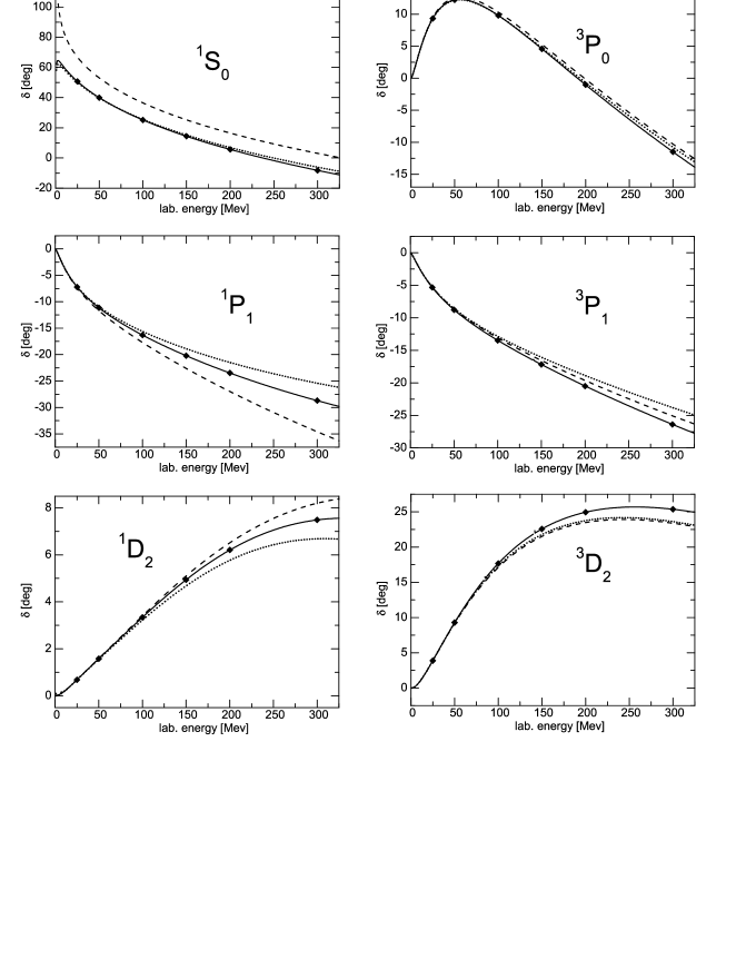
Figure 3: Neutron-proton phase parameters for the uncoupled partial waves, plotted versus the nucleon kinetic energy in the lab. system. Dashed[solid] curves calculated with Potential B parameters (Table 1) by solving Eqs. (66)[(71)]. Dotted represent the solutions of Eqs. (66) with UCT parameters (Table 1). The rhombs show original OBEP results (see Table 2).

However, a principal moment is to satisfy the requirement (86) for the Hamiltonian invariant under space inversion, time reversal and charge conjugation. A constructive consideration of the issue is given in Appendix  C.

Replacing in equations (67)–(69)

$$F^{2}_{b}[(p^{\prime}-p)^{2}]\left\{(p^{\prime}-p)^{2}-m_{b}^{2}\right\}^{-1}$$

by

$$-F^{2}_{b}[-(\vec{p}^{\prime}-\vec{p})^{2}]\left\{(\vec{p}^{\prime}-\vec{p})^{2}+m_{b}^{2}\right\}^{-1}$$

and neglecting the tensor-tensor term

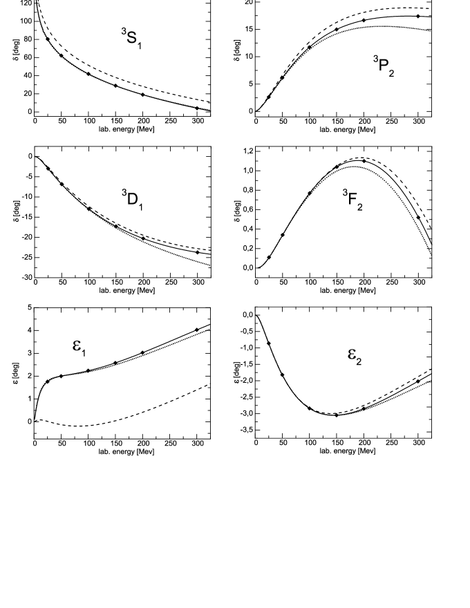
Figure 4: The same in Fig.3 but for the coupled waves.

$$\frac{{f_{\rm v}}^{2}}{4m^{2}}(E_{p^{\prime}}-E_{p})^{2}\bar{u}(\vec{p}^{\,\prime})[\gamma_{0}\gamma_{\nu}-g_{0\nu}]u(\vec{p})\\ \times\bar{u}(-\vec{p}^{\,\prime})[\gamma^{0}\gamma^{\nu}-g^{0\nu}]u(-\vec{p})$$ (70)

in (69), we obtain approximate expressions that with the common factor

$$(2\pi)^{-3}m^{2}/E_{p^{\prime}}E_{p}$$

instead of

$$(2\pi)^{-3}m/\sqrt{E_{p^{\prime}}E_{p}}$$

are equivalent to Eqs.(E.21)–(E.23) from MachHolElst87 . Such an equivalence becomes coincidence if in our formulae instead of the canonical two-nucleon basis $\left|{\vec{p}\,\mu_{1}\mu_{2}}\right\rangle$ one uses the helicity basis as in MachHolElst87 .

In parallel, we have considered the set of equations

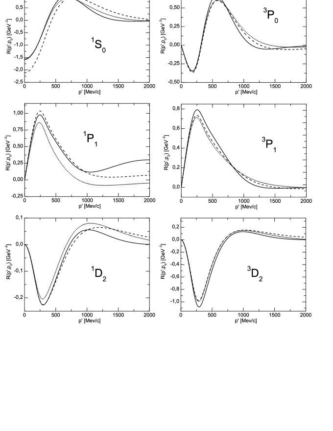
Figure 5: Half–off–shell $R$–matrices for uncoupled waves at laboratory energy equal to 150 MeV($p_{0}$=265 MeV). Other notations as in Fig.3

$${{}^{B}}R_{l^{\prime}{\rm{}}l}^{JST}(p^{\prime},p)={{}^{B}}V_{l^{\prime}{\rm{}}l}^{JST}(p^{\prime},p)\\ +m\sum\limits_{l^{\prime\prime}}\int\limits_{0}^{\infty}\frac{dq}{p^{2}-q^{2}}\left\{q^{2}\,{{}^{B}}V_{l^{\prime}l^{\prime\prime}}^{JST}(p^{\prime},q){{}^{B}}R_{l^{\prime\prime}l}^{JST}(q,p)\right.\\ \left.-p^{2}\,{{}^{B}}V_{l^{\prime}l^{\prime\prime}}^{JST}(p^{\prime},p){{}^{B}}R_{l^{\prime\prime}l}^{JST}(p,p)\right\},$$ (71)

where the superscript $B$ refers to the partial matrix elements of the potential $B$ determined in Mach89 with the just mentioned interchange of the bases. It is important to note that Eqs.(71) can be obtained from Eqs.(66) ignoring some relativistic effects. In particular, it means that the covariant OBE propagators

$$\frac{1}{{(p^{\prime}-p)^{2}-m_{b}^{2}}}=\frac{1}{(E_{p^{\prime}}-E_{p})^{2}-(\vec{p}^{\prime}-\vec{p})^{2}-m_{b}^{2}}$$ (72)

are replaced by their nonrelativistic counterparts

$$-\frac{1}{(\vec{p}^{\prime}-\vec{p})^{2}+m_{b}^{2}}$$ (73)

Such an approximation is a key point that gives rise to the potential $B$ from Mach89 .

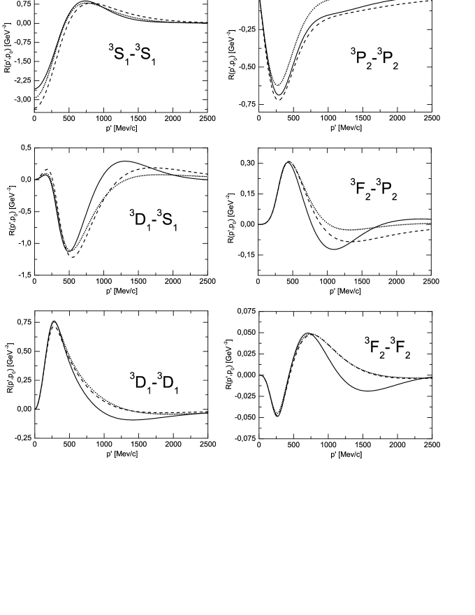
Figure 6: The same in Fig.5 but for the coupled waves.

However, the transition from (72) to (73), being valid on the energy shell

$$E_{p^{\prime}}=E_{p}=\frac{1}{2}E_{cms},$$ (74)

cannot be a priori justified when finding the $R$ matrix even on the shell. Thus our calculations of the $R$ matrices that meet the equations (66) and (71) are twofold. On the one hand, we will check reliability of our numerical procedure (in particular, its code). On the other hand, we would like to show similarities and discrepancies between our results and those by the Bonn group both on the energy shell and beyond it. These results are depicted in Figs. 3–8 and collected in Table 2.

As seen in Figs. 3–4, the most appreciable distinctions between the UCT and OBEP curves take place for the phase shifts with the lowest $l-$values. As the orbital angular momentum increases the difference between the solid and dashed curves decreases. Such features may be explained if one takes

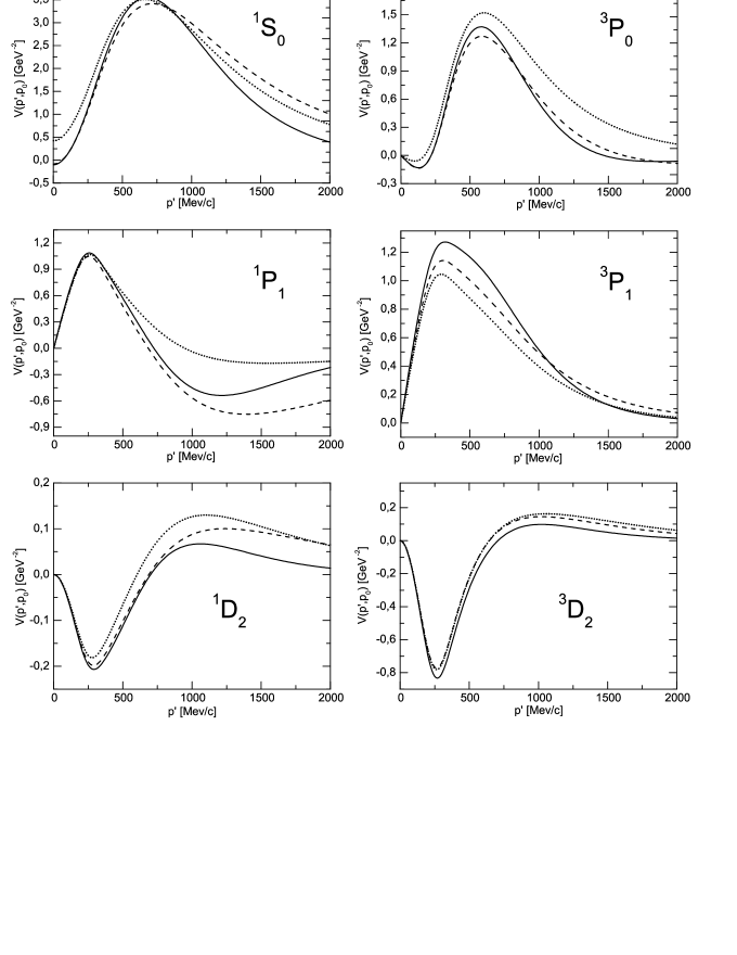
Figure 7: Potentials for the uncoupled partial waves with the momentum $p_{0}$ fixed as in Fig. 5. Other notations in Fig. 3.

into account that the approximations under consideration affect mainly high–momentum components of the UCT quasipotentials (their behavior at ”small” distances). With the $l$–increase the influence of small distances is suppressed by the centrifugal barrier repulsion.

Of course, it would be more instructive to compare the corresponding half–off–energy–shell $R$–matrices (see definition (51)). Their $p^{\prime}$–dependencies shown in Fig.5–6 are necessary to know when calculating the $\psi^{(\pm)}$ scattering states for a two–nucleon system. Such states may be expressed through the partial–wave functions $\varphi^{a}_{ll^{\prime}}\,\,a={J,S,T}$ that have the asymptotic of standing waves (see, for example, KorchinShebeko90 ). Within the MIM every $\varphi$ can be represented as

$$\varphi^{a}_{ll^{\prime}}(p)=\sum\limits_{j=1}^{N+1}B^{a}_{ll^{\prime}}(j)\delta(p-p_{j})/p^{2}_{j},$$

where the coefficients $B^{a}_{ll^{\prime}}(j)$ are the solutions of the set of linear algebraic equations

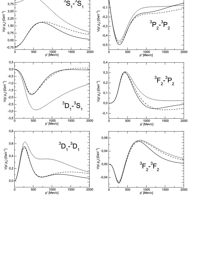
Figure 8: The same as in Fig.7 for the coupled waves.

approximately equivalent to the integral equation for the corresponding $R$–matrix; $N$ is the dimension of the set, $p_{j}$ are the grid points associated with the Gaussian nodes on the interval $[-1,1]$, $p_{N+1}=p_{0}$ (details can be found in KorchinShebeko90 ; LadyShe04 ). Meanwhile, our computations presented here have been done with $N=32$ (we do not talk about tests with other $N$-values to get the results stable with respect to $N$).

Completing the comparison of the UCT and Bonn results we display in Figs. 7–8 some interactions in relevant partial states. Appreciable distinctions between dotted and solid curves in these figures mean that the UCT and Bonn parameters from Table 1, ensuring a fair treatment of such on–energy–shell quantities as the phase shifts, may be inadequate in constructing model nucleon–nucleon potentials. It seems to be especially prominent in case of the ${}^{3}S_{1}-^{3}D_{1}$ potentials responsible for the formation of the tensor part of nuclear forces.

In addition, one should emphasize that hitherto we have explored the OBEP and UCT $R$–matrices in the c.m.s., where the both approaches yield the most close results. It is not the case in those situations when the c.m.s. cannot be referred to everywhere (e.g., in the reactions $NN\rightarrow\gamma NN$ and $\gamma d\rightarrow pn$). In this respect our studies of the differences between UCT and OBE approaches are under way.

5 Summary, Conclusions and Prospects

The present work has been made to develop a consistent field-theoretical approach in the theory of nucleon-nucleon scattering. It has been shown that the method of UCT’s, based upon the notion of clothed particles, is proved to be appropriate in achieving this purpose.

Starting from a primary Lagrangian for interacting meson and nucleon fields, we come to the corresponding Hamiltonian whose interaction part $K_{I}$ consists of new relativistic interactions responsible for physical (not virtual) processes in the system of the bosons ($\pi-$, $\eta-$, $\rho-$, $\omega-$, $\delta-$ and $\sigma-$mesons) and the nucleon. Proceeding with the CPR we have confined ourselves to constructing the four-legs interaction operators $K_{I}^{(2)}$ in the two-nucleon sector of the Hilbert space of hadronic states. The corresponding quasipotentials (these essentially nonlocal objects) for binary processes $NN\rightarrow NN$, $\bar{N}N\rightarrow\bar{N}N$, etc. are Hermitian and energy–independent. It makes them attractive for various applications in nuclear physics. They embody the off–shell effects in a natural way without addressing to any off–shell extrapolations of the $S-$matrix for the $NN$ scattering.

Using the unitary equivalence of the CPR to the BPR, we have seen how in the approximation $K_{I}=K_{I}^{(2)}$ the extremely complicated scattering problem in QFT can be reduced to the three –dimensional $LS$–type equation for the $T-$matrix in momentum space. The equation kernel is given by the clothed two-nucleon interaction of the class [2.2]. Such a conversion becomes possible owing to the property of $K_{I}^{(2)}$ to leave the two–nucleon sector and its separate subsectors to be invariant.

Special attention has been paid to the elimination of auxiliary field components. We encounter such a necessity for interacting vector and fermion fields when in accordance with the canonical formalism the interaction Hamiltonian density embodies not only a scalar contribution but nonscalar terms too. It has proved (at least, for the primary $\rho N$ and $\omega N$ couplings) that the UCT method allows us to remove such noncovariant terms directly in the Hamiltonian. To what extent this result will take place in higher orders in coupling constants it will be a subject of further explorations.

Being concerned with constructing the two–nucleon states from $\mathcal{H}$ and their angular–momentum decomposition we have not used the so–called separable ansatz, where every such state is a direct product of the corresponding one– nucleon (particle) states. The clothed two–nucleon partial waves have been built up as common eigenstates of the field total angular–momentum generator and its polarization (fermionic) part expressed through the clothed creation/destruction operators and their derivatives in momentum space.

We have not tried to attain a global treatment of modern precision data. But a fair agreement with the earlier analysis by the Bonn group makes sure that our approach may be useful for a more advanced analysis. In the context, to have a more convincing argumentation one needs to do at least the following. First, show the low-energy scattering parameters and the deuteron wave function calculated within the UCT method. Second, consider triple commutators $[R,[R,[R,V_{b}]]]$ to extract the two–boson–two–nucleon interaction operators of the same class [2.2] in the fourth order in the coupling constants. Third, extend our approach for describing the $NN$ scattering above the pion production threshold. All the things are in progress.

As a whole, the persistent clouds of virtual particles are no longer explicitly contained in the CPR, and their influence is included in the properties of the clothed particles (these quasiparticles of the UCT method). In addition, we would like to stress that the problem of the mass and vertex renormalizations is intimately interwoven with constructing the interactions between the clothed nucleons. The renormalized quantities are calculated step by step in the course of the clothing procedure unlike some approaches, where they are introduced by ”hands”.

6 Acknowledgements

We are thankful to V.Korda, who has allowed us to use an original code based upon a genetic algorithm for our best–fit procedure.

Appendix A Model Lagrangians and Hamiltonians within Canonical Formalism. Transition to Clothed Particle Representation

We will focused upon three boson fields (pseudoscalar, scalar and vector) that are coupled with the nucleon by means of the often employed interaction Lagrangians,

$$\mathscr{L}_{s}=-g_{s}^{0}\bar{\Psi}\Psi\Phi_{s},$$ (75)

$$\mathscr{L}_{ps}=-ig_{ps}^{0}\bar{\Psi}\gamma_{5}\Psi\Phi_{ps},$$ (76)

$$\mathscr{L}_{\rm{v}}=-g_{\rm{v}}^{0}\bar{\Psi}\gamma_{\mu}\Psi\Phi_{\rm{v}}^{\mu}-\frac{f_{\rm{v}}^{0}}{4m}\bar{\Psi}\sigma_{\mu\nu}\Psi\Phi_{\rm{v}}^{\mu\nu},$$ (77)

where $\sigma_{\mu\nu}=\frac{i}{2}(\gamma_{\mu}\gamma_{\nu}-\gamma_{\nu}\gamma_{\mu})$ and $\Phi_{\rm{v}}^{\mu\nu}=\partial^{\mu}\Phi_{\rm{v}}^{\nu}-\partial^{\nu}\Phi_{\rm{v}}^{\mu}$. As in Refs. (SheShi01 , KorCanShe07 ), throughout this paper we use the definitions and notations of BD , so, e.g., $\gamma_{\mu}\gamma_{\nu}+\gamma_{\nu}\gamma_{\mu}=2g_{\mu\nu}$ ($g_{00}=1$, $g_{11}=g_{22}=g_{33}=-1$), $\gamma_{\mu}^{{\dagger}}=\gamma_{0}\gamma_{\mu}\gamma_{0}$, $\gamma_{5}=i\gamma^{0}\gamma^{1}\gamma^{2}\gamma^{3}$. In addition, following Ref. WeinbergBook1995 we shall distinguish via upper(lower) case letters between the Heisenberg and Dirac picture field operators ($\Psi$ and $\Phi$ vs $\psi$ and $\varphi$, respectively, for fermions and bosons).

Of course, we could incorporate the so–called pseudovector (pv) coupling

$$\mathscr{L}_{pv}=-\frac{f_{pv}^{0}}{m_{ps}}\bar{\Psi}\gamma^{5}\gamma^{\mu}\Psi\partial_{\mu}\Phi_{ps}.$$ (78)

Since in this paper all used model interactions are suggested to be modified by introducing some cutoff factors, it has no matter that couplings (77) and (78) with derivatives are nonrenormalizable (cf. an instructive discussion of this subject in Subsect 3.4 of the survey Mach89 ). In the context, starting from couplings (75)–(77) with ”bare” constants $g_{ps}^{0}$, $g_{s}^{0}$, $g_{\rm{v}}^{0}$ and $f_{\rm{v}}^{0}$, we have tried to reproduce some results obtained in Refs. MachHolElst87 , Mach01 , where such constants from the beginning are replaced by effective parameters $g_{ps}$, $g_{s}$, $g_{\rm{v}}$ and $f_{\rm{v}}$. It explains (at least, ad hoc) our restriction to these Lagrangian densities. Recall also that for isospin 1 bosons one needs to write $\vec{\tau}\vec{\Phi}_{b}$ instead of $\Phi_{b}$, where $\vec{\tau}$ is the Pauli vector in isospin space.

In constructing the Hamiltonians with Lagrangian densities (75)–(77) as a departure point, we have first used the equations of motion for the $\rm{H}$ fields and the so–called Legendre transformation (from $L$ to $H$) to express the total Hamiltonian $H$ in terms of the independent canonical variables and their conjugates. Then, passing to the D picture (interaction representation) the Hamiltonian has been split into a physically satisfactory free–field part $H_{0}$ and an interaction $V$. Int. al., since the component $\Phi_{\rm{v}}^{0}$ has no canonical conjugate, we have resorted to a trick prompted by Eq.(7.5.22) from WeinbergBook1995 to introduce a proper component $\varphi_{\rm{v}}^{0}$ in the Dirac picture. As a result, we arrive to the interaction Hamiltonian densities:

$$\mathscr{H}_{s}(x)=g_{s}^{0}\bar{\psi}(x)\psi(x)\varphi_{s}(x),$$ (79)

$$\mathscr{H}_{ps}(x)=ig_{ps}^{0}\bar{\psi}(x)\gamma_{5}\psi(x)\varphi_{ps}(x),$$ (80)

$$\mathscr{H}_{\rm{v}}(x)=\mathscr{H}_{\rm{cov}}(x)+\mathscr{H}_{\rm{ncov}}(x),$$ (81)

where

$$\mathscr{H}_{\rm{cov}}(x)=g_{\rm{v}}^{0}\bar{\psi}(x)\gamma_{\mu}\psi(x)\varphi_{\rm{v}}^{\mu}(x)+\frac{f_{\rm{v}}^{0}}{4m}\bar{\psi}(x)\sigma_{\mu\nu}\psi(x)\varphi_{\rm{v}}^{\mu\nu}(x)$$ (82)

and

$$\mathscr{H}_{\rm{ncov}}(x)=\frac{g_{\rm{v}}^{0\,2}}{2m_{\rm{v}}^{2}}\bar{\psi}(x)\gamma_{0}\psi(x)\bar{\psi}(x)\gamma_{0}\psi(x)\\ +\frac{f_{\rm{v}}^{0\,2}}{4m^{2}}\bar{\psi}(x)\sigma_{0i}\psi(x)\bar{\psi}(x)\sigma_{0i}\psi(x).$$ (83)

It is implied that the total Hamiltonian of interest $H=H_{0}+V$ consists of the sum $H_{0}=H_{0,f}+\sum\limits_{b}H_{0,b}$, where $H_{0,f}$ the free–fermion Hamiltonian, $H_{0,b}$ separate free–boson contribution, and the space integral

$$V=\int d\vec{x}\mathscr{H}(\vec{x})$$ (84)

of the interaction density $\mathscr{H}(x)$ in the D picture

$$\mathscr{H}(x)=\mathscr{H}_{s}(x)+\mathscr{H}_{ps}(x)+\mathscr{H}_{\rm{v}}(x),$$ (85)

taken at $t=0$, i.e., in the Schrödinger (S) picture. In other words, $\mathscr{H}(\vec{x})=\mathscr{H}(0,\vec{x})$.

Expressions (79)-(84) exemplify that for a Lorentz–invariant Lagrangian it is not necessarily to have ”… the interaction Hamiltonian as the integral over space of a scalar interaction density; we also need to add non–scalar terms to the interaction density …” (quoted from p.292 of Ref. WeinbergBook1995 ). It is the case with derivative couplings and/or spin $\geq 1$.

In this connection, let us recall the property of the density $\mathscr{H}(x)$ to be scalar, viz.,

$$U_{F}(\Lambda,a)\mathscr{H}(x)U_{F}^{-1}(\Lambda,a)=\mathscr{H}(\Lambda x+a),$$ (86)

where the operators $U_{F}(\Lambda,a)$ realize a unitary irreducible representation of the Poincaré group in the Hilbert space of states for free (non–interacting) fields. Other comments will be given in Appendix B.

Moreover, it is well known that this property is a key point of covariant perturbation theory of the $S$–matrix (see, e.g., Chapter V of WeinbergBook1995 and refs. therein). In the respect, the division (81) is not accidental.

Further, the BPR form (1) and its comparison with Eq. (84) give rise to the interactions (3)–(5) between the bare bosons and fermions with physical masses. The next step is to apply the clothing procedure exposed in SheShi01 (see also KorCanShe07 ), where the first clothing transformation $W^{(1)}=\exp[R^{(1)}]$ (${R^{(1)}}^{{\dagger}}=-R^{(1)}$) eliminates all interactions linear in the coupling constants. Its generator $R^{(1)}$ obeys the equation

$$\left[R^{(1)},H_{F}\right]+V^{(1)}=0$$ (87)

with

$$V^{(1)}=V_{s}+V_{ps}+V_{\rm{v}}^{(1)},$$

where

$$V_{\rm{v}}^{(1)}=\int d\vec{x}\left\{g_{\rm{v}}\bar{\psi}(\vec{x})\gamma_{\mu}\psi(\vec{x})\varphi_{\rm{v}}^{\mu}(\vec{x})\phantom{\frac{f_{\rm{v}}}{4m}}\right.\\ \left.+\frac{f_{\rm{v}}}{4m}\bar{\psi}(\vec{x})\sigma_{\mu\nu}\psi(\vec{x})\varphi_{\rm{v}}^{\mu\nu}(\vec{x})\right\}.$$ (88)

Following SheShi01 Eq.(87) is satisfied with

$$R^{(1)}=-i\lim\limits_{\varepsilon\rightarrow 0+}\int\limits_{0}^{\infty}V_{D}^{(1)}(t)e^{-\varepsilon t}dt$$ (89)

if $m_{b}<2m$.

The corresponding interaction operator in the CPR (see relation (13) of the text) can be written as

$$K_{I}^{(2)}=\frac{1}{2}\left[R^{(1)},V^{(1)}\right]+V^{(2)},$$ (90)

where we have kept only the contributions of the second order in coupling constants, so

$$V^{(2)}=\int d\vec{x}\left\{\frac{g_{\rm{v}}^{2}}{2m_{\rm{v}}^{2}}\bar{\psi}(x\vec{)}\gamma_{0}\psi(\vec{x})\bar{\psi}(\vec{x})\gamma_{0}\psi(\vec{x})\right.\\ \left.+\frac{f_{\rm{v}}^{2}}{4m^{2}}\bar{\psi}(\vec{x})\sigma_{0i}\psi(\vec{x})\bar{\psi}(\vec{x})\sigma_{0i}\psi(\vec{x})\right\}$$ (91)

that coincides with the space integral of the non–scalar density $\mathscr{H}_{ncov}(x)$ at $t=0$. It is implied that all operators in the r.h.s. of Eq.(90) depend on the clothed–particle creation(destruction) operators $\alpha_{c}={W^{(1)}}^{{\dagger}}\alpha W^{(1)}$, for example, involved in the Fourier expansions

$$\psi(\vec{x})=(2\pi)^{-3/2}\int d\vec{p}\sqrt{\frac{m}{E_{\vec{p}}}}\sum\limits_{\mu}\left[u(\vec{p}\mu)b_{c}(\vec{p}\mu)\right.\\ \left.+v(-\vec{p}\mu)d_{c}^{{\dagger}}(-\vec{p}\mu)\right]\exp(i\vec{p}\vec{x}),$$

$$\varphi_{\rm{v}}^{\mu}(\vec{x})=(2\pi)^{-3/2}\int\frac{d\vec{k}}{\sqrt{2\omega_{\vec{k}}}}\sum\limits_{s}\left[e^{\mu}(\vec{k},s)a_{c}(\vec{k},s)\right.\\ \left.+e^{\mu}(-\vec{k},s)a_{c}^{{\dagger}}(-\vec{k},s)\right]\exp(i\vec{k}\vec{x}),$$

where the $e^{\mu}(\vec{k},s)$ for $s=+1,0,-1$ are three independent vectors, being transverse $k_{\mu}e^{\mu}(\vec{k},s)=0$, and normalized so that

$$\sum\limits_{s}e_{\mu}(\vec{k},s)e_{\nu}^{*}(\vec{k},s)=-g_{\mu\nu}+k_{\mu}k_{\nu}/m^{2}.$$

In this paper we do not intend to derive all interactions between the clothed mesons and nucleons, allowed by formula (90). Our aim is more humble, viz., to find in the r.h.s. of Eq.(90) terms of the type (18), responsible for the N–N interaction. Along the guideline the commutators $\frac{1}{2}[R^{(1)}_{s},V_{s}]$ and $\frac{1}{2}[R^{(1)}_{ps},V_{ps}]$ generate the scalar– and pseudoscalar–meson contributions $K_{b}(NN\rightarrow NN)$ with coefficients (20)–(21). In case of the vector mesons we encounter an interplay between the commutator $\frac{1}{2}[R^{(1)}_{\rm{v}},V_{\rm{v}}^{(1)}]$ and the integral (91).

To show it explicitly, let us write

$$V_{\rm{v}}^{(1)}=-\frac{1}{(2\pi)^{3/2}}\sum\limits_{\mu s}\int d\vec{k}d\vec{p}^{\prime}d\vec{p}\frac{m}{\sqrt{2\omega_{\vec{k}}E_{\vec{p}^{\prime}}E_{\vec{p}}}}e^{\rho}(\vec{k},s)\\ \times\delta\left(\vec{p}^{\,\prime}-\vec{p}-\vec{k}\right)\bar{u}(\vec{p}^{\,\prime}\mu^{\prime})\left\{{g_{\rm{v}}\gamma_{\rho}-\frac{f_{\rm{v}}}{2m}i\sigma_{\nu\rho}k^{\nu}}\right\}u(\vec{p}\mu)\\ \times b_{c}^{\dagger}(\vec{p}^{\prime}\mu^{\prime})b_{c}(\vec{p}\mu)a_{c}(\vec{k},s)+{\rm{H}}{\rm{.c}}.,$$ (92)

$$R_{\rm{v}}^{(1)}=-\frac{1}{(2\pi)^{3/2}}\sum\limits_{\mu s}\int d\vec{k}d\vec{p}^{\prime}d\vec{p}\frac{m}{\sqrt{2\omega_{\vec{k}}E_{\vec{p}^{\prime}}E_{\vec{p}}}}e^{\rho}(\vec{k},s)\\ \times\frac{\delta\left({\vec{p}^{\,\prime}-\vec{p}-\vec{k}}\right)}{E_{\vec{p}^{\prime}}-E_{\vec{p}}-\omega_{\vec{k}}}\bar{u}(\vec{p}^{\prime}\mu^{\prime})\left\{g_{\rm{v}}\gamma_{\rho}-\frac{f_{\rm{v}}}{2m}i\sigma_{\nu\rho}k^{\nu}\right\}u(\vec{p}\mu)\\ \times b_{c}^{\dagger}(\vec{p}^{\prime}\mu^{\prime})b_{c}(\vec{p}\mu)a_{c}(\vec{k},s)-{\rm{H}}{\rm{.c}}.,$$ (93)

retaining only those parts of $V^{(1)}$ and $R^{(1)}$, which are necessary for deriving $K_{\rm{v}}(NN\rightarrow NN)$. After a simple algebra we find

$$\frac{1}{2}\left[R^{(1)},V^{(1)}\right]_{\rm{v}}(NN\rightarrow NN)\\ =K_{\rm{v}}(NN\rightarrow NN)+K_{cont}(NN\rightarrow NN)$$

with

$$K_{\rm{v}}(NN\rightarrow NN)=\frac{1}{2(2\pi)^{3}}\sum\limits_{\mu}\int d\vec{p}^{\prime}_{1}d\vec{p}^{\prime}_{2}d\vec{p}_{1}d\vec{p}_{2}\\ \times\frac{m^{2}}{\sqrt{E_{\vec{p}^{\prime}_{1}}E_{\vec{p}^{\prime}_{2}}E_{\vec{p}_{1}}E_{\vec{p}_{2}}}}\frac{\delta\left({\vec{p}^{\,\prime}_{1}+\vec{p}^{\,\prime}_{2}-\vec{p}_{1}-\vec{p}_{2}}\right)}{(p_{1}^{\,\prime}-p_{1})^{2}-m_{b}^{2}}\\ \times\left[\bar{u}(\vec{p}_{1}^{\,\prime}\mu^{\prime}_{1})\left\{(g_{\rm{v}}+f_{\rm{v}})\gamma_{\nu}-\frac{f_{\rm{v}}}{2m}(p^{\prime}_{1}+p_{1})_{\nu}\right\}u(\vec{p}_{1}\mu_{1})\right.\\ \times\bar{u}(\vec{p}_{2}^{\,\prime}\mu^{\prime}_{2})\left\{(g_{\rm{v}}+f_{\rm{v}})\gamma^{\nu}-\frac{f_{\rm{v}}}{2m}(p^{\prime}_{2}+p_{2})^{\nu}\right\}u(\vec{p}_{2}\mu_{2})\\ -(E_{p^{\prime}_{1}}+E_{p^{\prime}_{2}}-E_{p_{1}}-E_{p_{2}})\\ \times\bar{u}(\vec{p}_{1}^{\,\prime}\mu^{\prime}_{1})\left\{(g_{\rm{v}}+f_{\rm{v}})\gamma_{\nu}-\frac{f_{\rm{v}}}{2m}(p^{\prime}_{1}+p_{1})_{\nu}\right\}u(\vec{p}_{1}\mu_{1})\\ \left.\times\bar{u}(\vec{p}_{2}^{\,\prime}\mu^{\prime}_{2})\frac{f_{\rm{v}}}{2m}\left\{\gamma^{0}\gamma^{\nu}-g^{0\nu}\right\}u(\vec{p}_{2}\mu_{2})\right]\\ \times b_{c}^{\dagger}(\vec{p}^{\,\prime}_{1}\mu^{\prime}_{1})b_{c}^{\dagger}(\vec{p}^{\prime}_{2}\mu^{\prime}_{2})b_{c}(\vec{p}_{1}\mu_{1})b_{c}(\vec{p}_{2}\mu_{2})$$

and

$$K_{cont}(NN\rightarrow NN)=\frac{1}{2(2\pi)^{3}}\sum\limits_{\mu}\int d\vec{p}^{\prime}_{1}d\vec{p}^{\prime}_{2}d\vec{p}_{1}d\vec{p}_{2}\\ \times\frac{m^{2}}{\sqrt{E_{\vec{p}^{\prime}_{1}}E_{\vec{p}^{\prime}_{2}}E_{\vec{p}_{1}}E_{\vec{p}_{2}}}}\delta\left(\vec{p}^{\,\prime}_{1}+\vec{p}^{\,\prime}_{2}-\vec{p}_{1}-\vec{p}_{2}\right)\\ \times\left[\frac{g_{\rm{v}}^{2}}{m_{\rm{v}}^{2}}\bar{u}(\vec{p}^{\,\prime}_{1}\mu^{\prime}_{1})\gamma_{0}u(\vec{p}_{1}\mu_{1})\bar{u}(\vec{p}^{\,\prime}_{2}\mu^{\prime}_{2})\gamma_{0}u(\vec{p}_{2}\mu_{2})\right.\\ \left.-\frac{f_{\rm{v}}^{2}}{4m^{2}}\bar{u}(\vec{p}^{\,\prime}_{1}\mu^{\prime}_{1})\gamma_{0}\vec{\gamma}u(\vec{p}_{1}\mu_{1})\bar{u}(\vec{p}^{\,\prime}_{2}\mu^{\prime}_{2})\gamma_{0}\vec{\gamma}u(\vec{p}_{2}\mu_{2})\right]\\ \times b_{c}^{\dagger}(\vec{p}^{\,\prime}_{1}\mu^{\prime}_{1})b_{c}^{\dagger}(\vec{p}^{\prime}_{2}\mu^{\prime}_{2})b_{c}(\vec{p}_{1}\mu_{1})b_{c}(\vec{p}_{2}\mu_{2})$$

The latter may be associated with a contact interaction since it does not contain any propagators (cf. the approach by the Osaka group TamuraSato88 ). It is easily seen that this operator cancels completely the non–scalar operator $V^{(2)}$. In other words the first UCT enables us to remove the non–invariant terms directly in the Hamiltonian. It gives an opportunity to work with the Lorentz scalar interaction only (at least, in the second order in the coupling constants). In our opinion, such a cancellation, first discussed here, is a pleasant feature of the CPR.

The remaining vector–meson contribution $K_{\rm{v}}(NN\rightarrow NN)$ is determined by coefficients (22) and gives us one more relativistic interaction in the boson–fermion system under consideration.

Appendix B Partial Wave Expansion of Two–Particles States in the CPR

We will show how one can proceed without the separable ansatz

$$\left|{\vec{p}_{1}\vec{p}_{2}\mu_{1}\mu_{2}}\right\rangle=\left|{\vec{p}_{1}\mu_{1}}\right\rangle\left|{\vec{p}_{2}\mu_{2}}\right\rangle$$

often exploited in relativistic quantum mechanics (RQM) (see, e.g., Werle66 and KeisPoly91 ) in getting expansions similar to Eq.(47). Unlike this, our consideration with particle creation/destruction as a milestone, where the clothed two–nucleon state is given by 

$$\left|{\vec{p}_{1}\mu_{1};\vec{p}_{2}\mu_{2}}\right\rangle=b_{c}^{\dagger}(p_{1}\mu_{1})b_{c}^{\dagger}(p_{2}\mu_{2})\left|\Omega\right\rangle$$ (94)

By definition, it belongs to the two–nucleon sector of $\mathscr{H}$ being the $K_{F}$ eigenstate with energy $E=p_{1}^{0}+p_{2}^{0}$. Moreover, it is assumed that vector $\left|\Omega\right\rangle$, being the single clothed no–particle state, has the property

$$U_{F}(\Lambda,a)\left|\Omega\right\rangle=\mathscr{P}\left|\Omega\right\rangle=\ldots=\left|\Omega\right\rangle$$ (95)

$$\forall\,\,\Lambda\in L_{+}\mbox{ and arbitrary spacetime shifts }a=(a^{0},\vec{a})$$

to be invariant with regard to the Poincaré group $\Pi$ , space inversion and other symmetries. Here $L_{+}$ is the homogeneous (proper) orthochronous Lorentz group. In turn, every $U_{F}(\Lambda,a)$ is expressed through the clothed free–particle generators of space–time translations

$$P_{F}^{\mu}(\alpha_{c})=\left\{{K_{F}(\alpha_{c}),\vec{P}_{F}(\alpha_{c})}\right\},$$

space rotations

$$\vec{J}_{F}(\alpha_{c})=\left\{{M_{F}^{23}(\alpha_{c}),M_{F}^{31}(\alpha_{c}),M_{F}^{12}(\alpha_{c})}\right\}$$

and the Lorentz boosts

$$\vec{B}_{F}(\alpha_{c})=\left\{{M_{F}^{01}(\alpha_{c}),M_{F}^{02}(\alpha_{c}),M_{F}^{03}(\alpha_{c})}\right\}$$

viz.,

$$U_{F}\left({\Lambda,a}\right)=\exp\left[{ia_{\rho}P_{F}^{\rho}(\alpha_{c})+\frac{i}{2}\omega_{\rho\nu}M_{F}^{\rho\nu}(\alpha_{c})}\right],$$ (96)

where the antisymmetric tensor $\omega_{\mu\nu}=-\omega_{\nu\mu}$ with $(\mu,\nu=0,1,2,3)$ has six independent components.

Now, let us remind of the following transformation property:

$$U_{F}\left({\Lambda,a}\right)b_{c}^{\dagger}\left({p\mu}\right)U_{F}^{-1}\left({\Lambda,a}\right)=e^{i\Lambda p\cdot a}b_{c}^{\dagger}\left({\Lambda p\mu^{\prime}}\right)D_{\mu^{\prime}\mu}^{(1/2)}\left({W\left({\Lambda,p}\right)}\right)$$ (97)

with the $D^{(1/2)}$ function whose argument is the Wigner rotation $W(\Lambda,p)$. The latter has the property $W(R,p)=R$ for any three–dimensional rotation $R$. In other words, from Eq.(97) it follows that under such a rotation, when $U_{F}(\Lambda,a)=U_{F}(R,0)\equiv U_{F}(R)$, one has

$$U_{F}\left({R}\right)b_{c}^{\dagger}\left({p\mu}\right)U_{F}^{-1}\left({R}\right)=b_{c}^{\dagger}\left({Rp\,\mu^{\prime}}\right)D_{\mu^{\prime}\mu}^{(1/2)}\left(R\right)$$ (98)

In addition, we need to have an analytic expression for the operator $\vec{J}_{ferm}$ to be expressed in terms of $b^{{\dagger}}_{c}$ and $b_{c}$. To do it we recur to the well known result:

$$\vec{J}_{ferm}=\int{d\vec{x}\psi^{\dagger}}(\vec{x})\left[{-i\vec{x}\times\frac{\partial}{{\partial\vec{x}}}+\frac{1}{2}\vec{\Sigma}}\right]\psi(\vec{x})$$ (99)

with $\vec{\Sigma}=\left({\begin{array}[]{*{20}c}{\vec{\sigma}}&0\\ 0&{\vec{\sigma}}\\ \end{array}}\right)$, where $\vec{\sigma}$ the Pauli vector.

After modest effort one can see that

$$\vec{J}_{ferm}=\vec{L}_{ferm}+\vec{S}_{ferm},$$ (100)

where $\vec{L}_{ferm}$ ($\vec{S}_{ferm}$) the orbital (spin) momentum of the fermion field, that are given by

$$\vec{L}_{ferm}=\frac{i}{2}\sum\limits_{\mu}{\int{d\vec{p}\,\,\vec{p}\times\left[\frac{\partial b_{c}^{\dagger}(\vec{p}\mu)}{\partial\vec{p}}b_{c}(\vec{p}\mu)-b_{c}^{\dagger}(\vec{p}\mu)\frac{{\partial b_{c}(\vec{p}\mu)}}{{\partial\vec{p}}}\right.}}\\ \left.+\frac{\partial d_{c}^{\dagger}(\vec{p}\mu)}{\partial\vec{p}}d_{c}(\vec{p}\mu)-d_{c}^{\dagger}(\vec{p}\mu)\frac{\partial d_{c}(\vec{p}\mu)}{\partial\vec{p}}\right]$$ (101)

and

$$\vec{S}_{ferm}=\frac{1}{2}\sum\limits_{\mu\mu^{\prime}}\int d\vec{p}\,\frac{m}{E_{\vec{p}}}\left[\left\{u^{\dagger}(\vec{p},\mu^{\prime})\vec{\Sigma}u(\vec{p},\mu)\phantom{\frac{1}{2}}\right.\right.\\ -\left.i\vec{p}\times\left(u^{\dagger}(\vec{p},\mu^{\prime})\frac{\partial u(\vec{p},\mu)}{\partial\vec{p}}-\frac{\partial u^{\dagger}(\vec{p},\mu^{\prime})}{\partial\vec{p}}u(\vec{p},\mu)\right)\right\}b_{c}^{\dagger}(\vec{p}\mu^{\prime})b_{c}(\vec{p}\mu)\\ -\left\{\upsilon^{\dagger}(\vec{p},\mu^{\prime})\vec{\Sigma}\upsilon(\vec{p},\mu)-i\vec{p}\times\left(\upsilon^{\dagger}(\vec{p},\mu^{\prime})\frac{\partial\upsilon(\vec{p},\mu)}{\partial\vec{p}}\phantom{\frac{1}{2}}\right.\right.\\ \left.\left.\left.-\frac{\partial\upsilon^{\dagger}(\vec{p},\mu^{\prime})}{\partial\vec{p}}\upsilon(\vec{p},\mu)\right)\right\}d_{c}^{\dagger}(\vec{p}\mu^{\prime})d_{c}(\vec{p}\mu)\right],$$

or

$$\vec{S}_{ferm}=\frac{1}{2}\sum\limits_{\mu\mu^{\prime}}\int d\vec{p}\,\,\chi^{{\dagger}}_{\mu^{\prime}}\vec{\sigma}\chi_{\mu}\left\{b_{c}^{\dagger}(\vec{p}\mu^{\prime})b_{c}(\vec{p}\mu)-d_{c}^{\dagger}(\vec{p}\mu^{\prime})d_{c}(\vec{p}\mu)\right\},$$ (102)

since

$${u^{\dagger}(\vec{p},\mu^{\prime})\frac{{\partial u(\vec{p},\mu)}}{{\partial\vec{p}}}-\frac{{\partial u^{\dagger}(\vec{p},\mu^{\prime})}}{{\partial\vec{p}}}u(\vec{p},\mu)}\\ ={\upsilon^{\dagger}(\vec{p},\mu^{\prime})\frac{{\partial\upsilon(\vec{p},\mu)}}{{\partial\vec{p}}}-\frac{{\partial\upsilon^{\dagger}(\vec{p},\mu^{\prime})}}{{\partial\vec{p}}}\upsilon(\vec{p},\mu)}\\ =\frac{i}{m(E_{p}+m)}\chi^{{\dagger}}_{\mu^{\prime}}\vec{\sigma}\chi_{\mu}\times\vec{p},$$

if one uses the Dirac spinors defined in BD . In these formulae we see the Pauli spinors $\chi_{\mu}$. It is important to keep in mind that

$$\vec{L}_{ferm}\neq-i\int{d^{3}x\psi^{\dagger}}(\vec{x})\vec{x}\times\frac{\partial}{{\partial\vec{x}}}\psi(\vec{x})$$

and

$$\vec{S}_{ferm}\neq\frac{1}{2}\int{d^{3}x\psi^{\dagger}(\vec{x})}\vec{\Sigma}\psi(\vec{x})$$

In fact, the operator $\vec{S}_{ferm}$ stems from a destructive interplay between orbital and spin parts of decomposition (99). In our opinion, such an interpretation differs from the definition below Eq.(13.48) in BD .

Hitherto, we have preserved the $\alpha_{c}$–dependence of the relevant operators although, as shown in Sect. 3 of SheShi01 , in the instant form of relativistic dynamics the operator $\vec{P}_{F}(\alpha_{c})(\vec{J}_{F}(\alpha_{c}))$ coincides with the total linear momentum $\vec{P}\equiv\vec{P}_{F}(\alpha)$ (the total angular momentum $\vec{J}\equiv\vec{J}_{F}(\alpha)$). Such an observation allows us to omit the label $c$ if it does not lead to confusion.

After these preliminaries we prefer to proceed sufficiently straightforwardly repeating the well known steps (cf. Werle66 and refs. therein). First, when handling the c.m.s. two–nucleon state

$$\left|{\vec{p}\mu_{1}\mu_{2}}\right\rangle=\left|{\vec{p}\mu_{1};-\vec{p}\mu_{2}}\right\rangle$$ (103)

let us consider the vector

$$\left|{\vec{p}SM_{S}}\right\rangle={\left({\left.\frac{1}{2}\mu_{1}\frac{1}{2}\mu_{2}\right|SM_{S}}\right)}\left|{\vec{p}\mu_{1}\mu_{2}}\right\rangle,$$ (104)

so

$$\left|{\vec{p}\mu_{1}\mu_{2}}\right\rangle={\left({\left.\frac{1}{2}\mu_{1}\frac{1}{2}\mu_{2}\right|SM_{S}}\right)}\left|{\vec{p}SM_{S}}\right\rangle$$ (105)

Second, one introduces

$$\left|{pJ(lS)M_{J}}\right\rangle=\int{d\hat{\vec{p}}}\,Y_{lm_{l}}\left(\hat{\vec{p}}\right)\left|{\vec{p}SM_{S}}\right\rangle\left({lm_{l}SM_{S}\left|{JM_{J}}\right.}\right)$$ (106)

or, reversely,

$$\left|{\vec{p}SM_{S}}\right\rangle=\left({lm_{l}SM_{S}\left|{JM_{J}}\right.}\right)Y_{lm_{l}}^{*}\left(\hat{\vec{p}}\right)\left|{pJ(lS)M_{J}}\right\rangle$$ (107)

with the unit vector $\hat{\vec{p}}=\vec{p}/p$.

Third, substituting (107) into the r.h.s. of Eq.(105) we arrive to the desired expansion,

$$\left|{\vec{p}\mu_{1}\mu_{2}}\right\rangle\\ ={\left({\left.\frac{1}{2}\mu_{1}\frac{1}{2}\mu_{2}\right|SM_{S}}\right)}\left({lm_{l}SM_{S}\left|{JM_{J}}\right.}\right)Y_{lm_{l}}^{*}\left(\hat{\vec{p}}\right)\left|{pJ(lS)M_{J}}\right\rangle$$ (108)

From the physical viewpoint it is important to know that

$${\vec{J}}^{\,2}\left|{pJ(lS)M_{J}}\right\rangle=J(J+1)\left|{pJ(lS)M_{J}}\right\rangle$$ (109)

$$J^{3}\left|{pJ(lS)M_{J}}\right\rangle=M_{J}\left|{pJ(lS)M_{J}}\right\rangle$$

and

$${\vec{S}}^{\,2}_{ferm}\left|{\vec{p}SM_{S}}\right\rangle=S(S+1)\left|{\vec{p}SM_{S}}\right\rangle$$ (110)

$$S_{ferm}^{3}\left|{\vec{p}SM_{S}}\right\rangle=M_{S}\left|{\vec{p}SM_{S}}\right\rangle$$

A simple way of deriving these relations is to use the transformation

$$U_{F}(R)|\vec{p}SM_{S}\rangle=|R\vec{p}SM_{S}^{\prime}\rangle D_{M_{S}^{\prime}M_{S}}^{(S)}(R)$$ (111)

$$\forall\,R\,\in\,\mbox{the rotation group}$$

and its consequence

$$U_{F}(R)|pJ(lS)M_{J}\rangle=|pJ(lS)M_{J}^{\prime}\rangle D_{M_{J}^{\prime}M_{J}}^{(J)}(R)$$ (112)

for infinitisemal rotations. With the help of (110) it is easily seen that

$${\vec{S}}^{\,2}_{ferm}\left|{pJ(lS)M_{J}}\right\rangle=S(S+1)\left|{pJ(lS)M_{J}}\right\rangle$$ (113)

Thus we have built up in the CPR the common eigenvectors of operators $\vec{J}^{2}$ and $\vec{S}_{ferm}^{2}$. Probably, one should note that $S$ is not any eigenvalue of the so–called invariant (or internal) spin operator $I=(0,\vec{I})$ introduced by M. Shirokov ChShir58 . While the latter involves internal orbital motion and polarization contributions, the quantum number $S$, whose values are regulated by Clebsch–Gordan coefficient in definition (104), characterizes rather the total spin of the two–nucleon system. Coming to the end, we allow ourselves to write the parity operator of the fermion (nucleon) field in the CPR (cf. Eq.(15.93) from BD ):

$$\mathscr{P}_{ferm}=exp[i\pi_{ferm}],$$

$$\pi_{ferm}=-\frac{\pi}{2}\int d^{3}p\left[b_{c}^{{\dagger}}(\vec{p}\mu)b_{c}(\vec{p}\mu)-b_{c}^{{\dagger}}(\vec{p}\mu)b_{c}(-\vec{p}\mu)\right.\\ \left.+d_{c}^{{\dagger}}(\vec{p}\mu)d_{c}(\vec{p}\mu)+d_{c}^{{\dagger}}(\vec{p}\mu)d_{c}(-\vec{p}\mu)\right]$$ (114)

with the relations

$$\mathscr{P}_{ferm}b_{c}(\vec{p}\mu)\mathscr{P}_{ferm}^{-1}=b_{c}(-\vec{p}\mu),$$

$$\mathscr{P}_{ferm}d^{{\dagger}}_{c}(\vec{p}\mu)\mathscr{P}_{ferm}^{-1}=-d^{{\dagger}}_{c}(-\vec{p}\mu)$$

that extend the rules (97) for the clothed particle operators to such an improper transformation as the space inversion.

Appendix C The Regularized Quasipotentials and their Angular–Momentum Decomposition

Trying to overcome ultraviolet divergences inherent in solving equation (50), we will regularize their driving terms by introducing some cutoff factors. It can be achieved if instead of Eq.(19) one assumes

$$V_{b}^{reg}(p_{1}^{\prime}\mu_{1}^{\prime},p_{2}^{\prime}\mu_{2}^{\prime};p_{1}\mu_{1},p_{2}\mu_{2})=\frac{\delta\left(\vec{p}_{1}^{\,\prime}+\vec{p}_{2}^{\,\prime}-\vec{p}_{1}-\vec{p}_{2}\right)}{\sqrt{p_{01}^{\prime}p_{02}^{\prime}p_{01}p_{02}}}\\ v_{b}^{reg}(p_{1}^{\prime}\mu_{1}^{\prime},p_{2}^{\prime}\mu_{2}^{\prime};p_{1}\mu_{1},p_{2}\mu_{2})$$ (115)

omitting for the moment isospin indices, so

$$K_{b}(NN\rightarrow NN)\rightarrow K_{b}^{reg}(NN\rightarrow NN)\\ =\int\delta\left(\vec{p}_{1}^{\,\prime}+\vec{p}_{2}^{\,\prime}-\vec{p}_{1}-\vec{p}_{2}\right)\frac{d\vec{p}_{1}^{\,\prime}}{p_{01}^{\prime}}\frac{d\vec{p}_{2}^{\,\prime}}{p_{02}^{\prime}}\frac{d\vec{p}_{1}}{p_{01}}\frac{d\vec{p}_{2}}{p_{02}}\\ \sum\limits_{\mu}v_{b}^{reg}(p_{1}^{\prime}\mu_{1}^{\prime},p_{2}^{\prime}\mu_{2}^{\prime};p_{1}\mu_{1},p_{2}\mu_{2})\\ b_{c}^{{\dagger}}(p_{1}^{\prime}\mu_{1}^{\prime})b_{c}^{{\dagger}}(p_{2}^{\prime}\mu_{2}^{\prime})b_{c}(p_{1}\mu_{1})b_{c}(p_{2}\mu_{2})$$ (116)

Here the new (regularized) coefficients $v_{b}^{reg}$ are given by

$$v_{b}^{reg}=F_{b}(p_{1}^{\prime},p_{2}^{\prime};p_{1},p_{2})v_{b},$$ (117)

where the old ones $v_{b}$ are determined by Eq.(20)–(22) and empirical cutoff functions $F_{b}$ should not violate the known symmetries of interactions. In particular, if one writes

$$K_{b}^{reg}(NN\rightarrow NN)=\int K_{b}^{reg}(\vec{x})d\vec{x}$$ (118)

with

$$K_{b}^{reg}(\vec{x})=\frac{1}{(2\pi)^{3}}\int\frac{d\vec{p}_{1}^{\,\prime}}{p_{01}^{\prime}}\frac{d\vec{p}_{2}^{\,\prime}}{p_{02}^{\prime}}\frac{d\vec{p}_{1}}{p_{01}}\frac{d\vec{p}_{2}}{p_{02}}d\vec{x}e^{i\left(\vec{p}_{1}^{\,\prime}+\vec{p}_{2}^{\,\prime}-\vec{p}_{1}-\vec{p}_{2}\right)\vec{x}}\\ \sum\limits_{\mu}v_{b}^{reg}(p_{1}^{\prime}\mu_{1}^{\prime},p_{2}^{\prime}\mu_{2}^{\prime};p_{1}\mu_{1},p_{2}\mu_{2})\\ b_{c}(p_{1}^{\prime}\mu_{1}^{\prime})b_{c}(p_{2}^{\prime}\mu_{2}^{\prime})b_{c}^{{\dagger}}(p_{1}\mu_{1})b_{c}^{{\dagger}}(p_{2}\mu_{2})$$ (119)

then the RI implies the property of the operator

$$K_{b}^{reg}(x)\equiv\exp\left(iK_{F}t\right)K_{b}^{reg}(\vec{x})\exp\left(-iK_{F}t\right)$$ (120)

to be a scalar, viz.,

$$U_{F}(\Lambda,\lambda)K_{b}^{reg}(x)U_{F}^{-1}(\Lambda,\lambda)=K_{b}^{reg}(\Lambda x+\lambda)$$ (121)

But accordingly (97) it imposes the following restrictions

$$D_{\eta_{1}^{\prime}\mu_{1}^{\prime}}^{\left(\frac{1}{2}\right)}\left(W(\Lambda,p_{1}^{\prime})\right)D_{\eta_{2}^{\prime}\mu_{2}^{\prime}}^{\left(\frac{1}{2}\right)}\left(W(\Lambda,p_{2}^{\prime})\right)\\ \times D_{\eta_{1}\mu_{1}}^{\left(\frac{1}{2}\right)\ast}\left(W(\Lambda,p_{1})\right)D_{\eta_{2}\mu_{2}}^{\left(\frac{1}{2}\right)\ast}\left(W(\Lambda,p_{2})\right)\\ \times v_{b}^{reg}(p_{1}^{\prime}\mu_{1}^{\prime},p_{2}^{\prime}\mu_{2}^{\prime};p_{1}\mu_{1},p_{2}\mu_{2})=\\ v_{b}^{reg}(\Lambda p_{1}^{\prime}\eta_{1}^{\prime},\Lambda p_{2}^{\prime}\eta_{2}^{\prime};\Lambda p_{1}\eta_{1},\Lambda p_{2}\eta_{2})$$ (122)

to the coefficients $v_{b}^{reg}$. In this connection, before going on, one needs to verify that the old (non–regularized) ones satisfy relation (122) themselves. It can be done with the help of the property

$$S(\Lambda)u(p\mu)=D_{\mu^{\prime}\mu}^{(1/2)}(W(\Lambda,p))u(\Lambda p\mu^{\prime}),$$

where $S(\Lambda)=exp\left[-\frac{1}{2}\omega_{\mu\nu}\sigma^{\mu\nu}\right]$ the matrix of the nonunitary representation $\Lambda\rightarrow S(\Lambda)$ in the space of spinor indices. Indeed, recalling more the relations

$$S(\Lambda)^{-1}\gamma^{\rho}S(\Lambda)=\gamma^{\mu}\Lambda^{\rho}_{\,\,\mu},$$

one can easily seen that the quantities $v_{b}(p_{1}^{\prime}\mu_{1}^{\prime},p_{2}^{\prime}\mu_{2}^{\prime};p_{1}\mu_{1},p_{2}\mu_{2})=v_{b}(1^{\prime},2^{\prime};1,2)$ by Eqs.(20)–(22) obey Eq.(122). Also, let us remind (see, e.g., MelShe ) that for a Lorentz boost $\Lambda=L(\vec{v})$ with the velocity $\vec{v}$, the Wigner transformation $W(\Lambda,p)$ is the rotation about the $\vec{v}\times\vec{p}$ –direction by an angle $\psi$, which can be represented as

$$m\left(1+\gamma+\frac{p_{0}^{\star}}{m}+\frac{p_{0}}{m}\right)\tan\frac{\psi}{2}=\gamma\left|\vec{v}\times\vec{p}\right|,$$

where $p_{0}^{\star}$ the zeroth component of the nucleon momentum $p^{\star}=(p_{0}^{\star},\vec{p}^{\,\star})=L(\vec{v})p$ in the moving frame and $\gamma$ the corresponding Lorentz factor. As noted, $W(R,p)=R$ for a pure rotation $R$.

Now, keeping in mind the relation (117) we need to deal with a Lorentz–invariant cutoff,

$$F_{b}(p_{1}^{\prime},p_{2}^{\prime};p_{1},p_{2})=F_{b}(\Lambda p_{1}^{\prime},\Lambda p_{2}^{\prime};\Lambda p_{1},\Lambda p_{2})$$ (123)

in our model regularization,

$$V_{b}^{reg}(p_{1}^{\prime}\mu_{1}^{\prime},p_{2}^{\prime}\mu_{2}^{\prime};p_{1}\mu_{1},p_{2}\mu_{2})=\frac{\delta\left(\vec{p}_{1}^{\,\prime}+\vec{p}_{2}^{\,\prime}-\vec{p}_{1}-\vec{p}_{2}\right)}{\sqrt{p_{01}^{\prime}p_{02}^{\prime}p_{01}p_{02}}}\\ F_{b}(p_{1}^{\prime},p_{2}^{\prime};p_{1},p_{2})v_{b}(p_{1}^{\prime}\mu_{1}^{\prime},p_{2}^{\prime}\mu_{2}^{\prime};p_{1}\mu_{1},p_{2}\mu_{2})$$ (124)

Further, assuming that $F_{b}$ depends on the two invariants $(p_{1}-p_{1}^{\prime})^{2}$ and $(p_{2}-p_{2}^{\prime})^{2}$,

$$F_{b}(p_{1}^{\prime},p_{2}^{\prime};p_{1},p_{2})=f_{b}\left((p_{1}-p_{1}^{\prime})^{2},(p_{2}-p_{2}^{\prime})^{2}\right)$$

we have on the momentum shell,

$$(p_{1}-p_{1}^{\prime})^{2}=(E_{1}-E_{1}^{\prime})^{2}-(\vec{p}_{1}-\vec{p}_{1}^{\,\prime})^{2}$$

$$(p_{2}-p_{2}^{\prime})^{2}=(E_{2}-E_{2}^{\prime})^{2}-(\vec{p}_{1}-\vec{p}_{1}^{\,\prime})^{2}$$

so in the c.m.s. one has to deal with the function $f_{b}[(p-p^{\prime})^{2}]$ ($F^{2}_{b}\left[(p^{\prime}-p)^{2}\right]$ in the main text) of one invariant $(p-p^{\prime})^{2}=(E_{\vec{p}}-E_{\vec{p}^{\,\prime}})^{2}-(\vec{p}-\vec{p}^{\,\prime})^{2}$.

Of course, a similar regularization could be implemented if the vertices

$$\bar{u}(p^{\prime}\mu^{\prime})\Gamma_{b}(k)u(p\mu)$$

(see, e.g., Eq.(92)) would be at the beginning modified by introducing cutoff factors $g_{++}^{b}(p^{\prime},p)$ with the bosons and fermions on their mass shells $k^{2}=m_{b}^{2}$, $p^{\prime 2}=p^{2}=m^{2}$ and the momentum conservation $\vec{k}=\vec{p}^{\prime}-\vec{p}$. Neglecting a possible dependence of such factors on particle polarizations, we preserve the subscript $++$ keeping in mind a more symmetrical consideration, where some factors $g_{\varepsilon^{\prime}\varepsilon}^{b}(p^{\prime},p)$ could be introduced with the proper energy–sign labels $\varepsilon^{\prime}$ and $\varepsilon$ for separate three–legs contributions to a given boson–fermion Yukawa–type interaction. Then the corresponding regularized quasipotentials would be contained factors

$$F_{b}(p_{1}^{\prime},p_{2}^{\prime};p_{1},p_{2})=g_{++}^{b}(p_{1}^{\prime},p_{1})g_{++}^{b}(p_{2},p_{2}^{\prime})$$ (125)

in the quadrilinear terms.

As noted below Eq.(66) our choice of the phenomenological cutoff $F_{b}[(p^{\prime}-p)^{2}]$ has been prompted by those investigations MachHolElst87 of the Bonn group. Of course, recent developments in studying the structure of meson–baryon interaction vertices are of great interest. Among certain achievements in this area we find a microscopic derivation of the strong $\pi NN$ and $\pi N\Delta$ FFs within the quark model developed by the Graz group (see, e.g., Graz ). Being free of any phenomenological input (fit parameters) the corresponding prediction for the FF $G_{\pi NN}$ (e.g., in an analytic form put forward in Graz ) could be employed as the bare factor $g^{\pi}_{++}(p^{\prime},p)$. The latter has the property $g^{\pi}_{++}(\Lambda p^{\prime},\Lambda p)=g^{\pi}_{++}(p^{\prime},p)$, i.e., it should be dependent upon the Lorentz scalar $p^{\prime}p$ or $(p^{\prime}-p)^{2}$ to fulfill condition (86). Other vertex cutoffs $g^{\pi}_{+-}$, $g^{\pi}_{-+}$ and $g^{\pi}_{--}$ are also desirable to be introduced on the same physical footing.

By the way, along with properties $g^{b}_{\pm\pm}(\Lambda p^{\prime},\Lambda p)=g^{b}_{\pm\pm}(p^{\prime},p)$ condition (86) means that the crossed cutoffs $g^{b}_{+-}(p^{\prime},p)$ and $g^{b}_{-+}(p^{\prime},p)$ should be some functions of the four–product $p^{\prime}_{-}p=p^{\prime}p_{-}$. In turn, other symmetries, mentioned below Eq.(69), yield the following links $g^{b}_{\varepsilon^{\prime}\varepsilon}(p^{\prime},p)=g^{b}_{\varepsilon^{\prime}\varepsilon}(p,p^{\prime})$, $g^{b}_{++}(p^{\prime},p)=g^{b}_{--}(p^{\prime},p)$, $g^{b}_{+-}(p^{\prime},p)=g^{b}_{-+}(p,p^{\prime})$ for the real functions. All the things are extremely important for constructing a relativistic nonlocal QFT, where the boosts operators are determined as elements of the Lie algebra of the Poincaré group. It will be presented somewhere else.

In addition, let us address the matrix elements $\langle p^{\prime}\mid j_{b}(0)\mid p\rangle$ that are closely connected with the FFs in question (see, e.g., Gas66 ) since we handle the corresponding baryon current density $j_{b}(x)$ at $x=0$ sandwiched between physical (clothed) one–nucleon states. Such matrix elements might be evaluated in terms of the cutoffs and other physical inputs using some idea from SheShi00 (cf. the clothed particle representation of a current operator therein). From the constructive point of view, it means the use of definitions $\mid p\rangle=b_{c}^{{\dagger}}(p\mu)\mid\Omega\rangle$ and $\mid p^{\prime}\rangle=b_{c}^{{\dagger}}(p^{\prime}\mu^{\prime})\mid\Omega\rangle$, adopted at the beginning of Appendix B, and the similarity transformation

$$j_{b}(0)=e^{R(\alpha_{c})}j_{b}^{c}(0)e^{-R(\alpha_{c})}\\ =j_{b}^{c}(0)+\left[R(\alpha_{c}),j_{b}^{c}(0)\right]+\frac{1}{2!}\left[R(\alpha_{c}),\left[R(\alpha_{c}),j_{b}^{c}(0)\right]\right]\\ +\frac{1}{3!}\left[R(\alpha_{c}),\left[R(\alpha_{c}),\left[R(\alpha_{c}),j_{b}^{c}(0)\right]\right]\right]+\cdots,$$

where $j_{b}^{c}(0)$ is the same current density but expressed through the clothed operators. The nonperturbative expansion in the commutators gives an opportunity for a systematic evaluation of corrections to matrix elements

$$\langle\Omega\mid b_{c}j_{b}^{c}(0)b_{c}^{{\dagger}}\mid\Omega\rangle=\langle\Omega_{0}\mid bj_{b}(0)b^{{\dagger}}\mid\Omega_{0}\rangle.$$

Some simplifications originate from the well–known fact that similar expectations of the commutators that involve odd number of meson operators are equal to zero.

In general, one can elaborate a recursive procedure of calculations, like that by Kharkov-Padova group, for manipulations with the multiple commutators $[V]^{n}$ ($n=2,3,\cdots$) (see KorCanShe07 ). Doing so, one can find corrections to formula (125) obtained from the commutator $[V]^{1}=[R,V]$. This work is in progress.

After this prelude we note that the partial–wave matrix elements of interest are defined by

$$\bar{V}_{l^{\prime}l}^{JS}=\sum\limits_{b}{{}^{b}}\bar{V}_{l^{\prime}l}^{JS}=\frac{1}{2J+1}\sum\limits_{b}\int d\hat{\vec{p}^{\prime}}\int d\hat{\vec{p}}\,\,Y_{l^{\prime}m_{l}^{\prime}}^{\ast}(\hat{\vec{p}^{\prime}})Y_{lm_{l}}(\hat{\vec{p}})\\ \left(l^{\prime}m_{l}^{\prime}SM_{S}^{\prime}\left|JM_{J}\right.\right)\left(lm_{l}SM_{S}\left|JM_{J}\right.\right)\langle\left.\vec{p}^{\,\prime}SM_{S}^{\prime}\right|\bar{V}_{b}\left|\vec{p}SM_{S}\right.\rangle$$ (126)

with

$$\langle\left.\vec{p}^{\,\prime}SM_{S}^{\prime}\right|\bar{V}_{b}\left|\vec{p}SM_{S}\right.\rangle=\\ \bar{V}_{dir}^{b}(\vec{p}^{\,\prime}SM_{S}^{\prime},\vec{p}SM_{S})-\bar{V}_{exc}^{b}(\vec{p}^{\,\prime}SM_{S}^{\prime},\vec{p}SM_{S}),$$ (127)

$$\bar{V}_{dir(exc)}^{b}(\vec{p}^{\,\prime}SM_{S}^{\prime},\vec{p}SM_{S})=-\frac{1}{2(2\pi)^{3}}\frac{m^{2}}{E_{p^{\prime}}E_{p}}\\ \left(\frac{1}{2}\mu_{1}^{\prime}\frac{1}{2}\mu_{2}^{\prime}\left|SM_{S}^{\prime}\right.\right)\left(\frac{1}{2}\mu_{1}\frac{1}{2}\mu_{2}\left|SM_{S}\right.\right)v_{b}^{dir(exc)}(\vec{p}^{\,\prime}\mu_{1}^{\prime}\mu_{2}^{\prime},\vec{p}\mu_{1}\mu_{2}),$$ (128)

where we have employed formula (45) and property (48).
In turn, the matrices $v_{b}^{dir}(\vec{p}^{\,\prime}\mu_{1}^{\prime}\mu_{2}^{\prime},\vec{p}\mu_{1}\mu_{2})$ can be represented as

$$v_{b}^{dir}=\Gamma_{b}(\vec{p}^{\,\prime}\mu_{1}^{\prime};\vec{p}\mu_{1})D_{b}(p^{\prime},p)\Gamma_{b}(-\vec{p}^{\,\prime}\mu_{2}^{\prime};-\vec{p}\mu_{2}),$$ (129)

$$D_{b}(p^{\prime},p)=\frac{F^{2}_{b}\left[(p^{\prime}-p)^{2}\right]}{(p^{\prime}-p)^{2}-m_{b}^{2}}.$$ (130)

Recall that

$$v_{b}^{exc}(\vec{p}^{\,\prime}\mu_{1}^{\prime}\mu_{2}^{\prime},\vec{p}\mu_{1}\mu_{2})=v_{b}^{dir}(\vec{p}^{\,\prime}\mu_{1}^{\prime}\mu_{2}^{\prime},-\vec{p}\mu_{2}\mu_{1}),$$

so

$$\bar{V}_{exc}^{b}(\vec{p}^{\,\prime}SM_{S}^{\prime},\vec{p}SM_{S})=(-1)^{S+1}\bar{V}_{dir}^{b}(\vec{p}^{\,\prime}SM_{S}^{\prime},-\vec{p}SM_{S}).$$ (131)

Further, taking into account the completeness of the matrices ${1,\vec{\sigma}}$ in $2\times 2$ space, the non–regularized vertices from Eqs.(20)–(22) can be written as

$$\Gamma_{b}(\vec{p}^{\,\prime}\mu^{\prime};\vec{p}\mu)=A_{b}(\vec{p}^{\,\prime};\vec{p})\delta_{\mu^{\prime}\mu}+\mbox{ a linear functional of }\vec{\sigma}$$

Now, to get the matrix $\langle\left.\vec{p}^{\,\prime}SM_{S}^{\prime}\right|\bar{V}_{b}\left|\vec{p}SM_{S}\right.\rangle$ we could do all summations in formula (128) over $\mu$ projections directly. However, we prefer the following way putting formally

$$\langle\mu_{1}^{\prime}|\vec{\sigma}|\mu_{1}\rangle=\langle\mu_{1}^{\prime}|\hat{\vec{\sigma}}(1)|\mu_{1}\rangle\,\,\,\,\mbox{and}\,\,\,\,\langle\mu_{2}^{\prime}|\vec{\sigma}|\mu_{2}\rangle=\langle\mu_{2}^{\prime}|\hat{\vec{\sigma}}(2)|\mu_{2}\rangle$$

to obtain

$$\bar{V}_{dir}^{b}(\vec{p}^{\,\prime}SM_{S}^{\prime},\vec{p}SM_{S})=\langle\left.SM_{S}^{\prime}\right|G_{b}(\vec{p}^{\,\prime},\vec{p};\hat{\vec{\sigma}}(1),\hat{\vec{\sigma}}(2))\left|SM_{S}\right.\rangle$$ (132)

with the $SM_{S}$ eigenvalue equations,

$$\hat{\vec{S}}^{2}|SM_{S}\rangle=S(S+1)|SM_{S}\rangle$$

$$\hat{S}_{3}|SM_{S}\rangle=M_{S}|SM_{S}\rangle,$$

where $\hat{\vec{S}}=\frac{1}{2}\left[\hat{\vec{\sigma}}(1)+\hat{\vec{\sigma}}(2)\right]$. The operators $G_{b}$ can be expressed through the operator $\hat{\vec{S}}$ with the help of the relations

$$\hat{\vec{\sigma}}(1)\cdot\vec{n}\,\,\,\hat{\vec{\sigma}}(2)\cdot\vec{n}=2\left(\hat{\vec{S}}\cdot\vec{n}\right)^{2}-\vec{n}^{2}$$

$$\hat{\vec{\sigma}}(1)\times\vec{n}\,\,\,\hat{\vec{\sigma}}(2)\times\vec{n}=\hat{\vec{\sigma}}(1)\cdot\hat{\vec{\sigma}}(2)\,\,\,\vec{n}^{2}-\hat{\vec{\sigma}}(1)\cdot\vec{n}\,\,\,\hat{\vec{\sigma}}(2)\cdot\vec{n}$$

for any vector $\vec{n}$.
As a result, we find with the models (20)–(22)

$$G_{s}=\frac{g_{s}^{2}}{2(2\pi)^{3}}CD_{s}(p^{\prime},p)\left\{U_{1}^{2}+\vec{V}_{3}^{2}-2(\vec{V}_{3}\vec{S})\left[iU_{1}+(\vec{V}_{3}\vec{S})\right]\right\},$$ (133)

$$G_{ps}=\frac{g_{ps}^{2}}{2(2\pi)^{3}}CD_{ps}(p^{\prime},p)\left\{\vec{V}_{1}^{2}-2(\vec{V}_{1}\vec{S})^{2}\right\},$$ (134)

$$G_{\rm{v}}=G_{\rm{v}}^{vv}+G_{\rm{v}}^{vt}+G_{\rm{v}}^{tt},$$ (135)

$$G_{\rm{v}}^{vv}=\frac{g_{\rm{v}}^{2}}{2(2\pi)^{3}}CD_{\rm{v}}(p^{\prime},p)G_{1},$$ (136)

$$G_{\rm{v}}^{vt}=\frac{1}{2(2\pi)^{3}}\frac{f_{\rm{v}}g_{\rm{v}}}{2m}CD_{\rm{v}}(p^{\prime},p)\left\{4mG_{1}\right.\\ \left.-2\left[(E_{p^{\prime}}+E_{p})G_{2}+G_{3}+(E_{p^{\prime}}-E_{p})G_{4}\right]\right\},$$ (137)

$$G_{\rm{v}}^{tt}=\frac{1}{2(2\pi)^{3}}\frac{f_{\rm{v}}^{2}}{4m^{2}}CD_{\rm{v}}(p^{\prime},p)\left\{4m^{2}G_{1}\right.\\ -4m\left[(E_{p^{\prime}}+E_{p})G_{2}+G_{3}+(E_{p^{\prime}}-E_{p})G_{4}\right]\\ \left.+G_{5}+2(E_{p^{\prime}}-E_{p})G_{6}\right\},$$ (138)

with

$$G_{1}=U_{2}^{2}+\vec{V}_{3}^{2}+\vec{V}_{2}^{2}-2(\vec{S}^{2}-1)\vec{V}_{1}^{2}\\ +2(\vec{V}_{3}\vec{S})\left[iU_{2}-(\vec{V}_{3}\vec{S})\right]+2(\vec{V}_{1}\vec{S})^{2}+2i(\vec{V}_{2}\times\vec{V}_{1})\vec{S},$$

$$G_{2}=U_{1}U_{2}-\vec{V}_{3}^{2}+2(\vec{V}_{3}\vec{S})\left[i(U_{1}-U_{2})+2(\vec{V}_{3}\vec{S})\right],$$

$$G_{3}=U_{1}\vec{B}\vec{V}_{2}+i(\vec{B}\vec{V}_{2})(\vec{V}_{3}\vec{S})+iU_{1}(\vec{B}\times\vec{V}_{1})\vec{S}\\ -(\vec{B}\times\vec{V}_{1})\left[2\vec{S}(\vec{V}_{3}\vec{S})-\vec{V}_{3}-i(\vec{V}_{3}\times\vec{S})\right],$$

$$G_{4}=(5-2\vec{S}^{2})\vec{V}_{1}\vec{V}_{2}+(\vec{V}_{1}\vec{S})(\vec{V}_{2}\vec{S})+(\vec{V}_{2}\vec{S})(\vec{V}_{1}\vec{S}),$$

$$G_{5}=\vec{B}^{2}\left\{U_{1}^{2}+\vec{V}_{3}^{2}+2(\vec{V}_{3}\vec{S})\left[iU_{1}-(\vec{V}_{3}\vec{S})\right]\right\},$$

$$G_{6}=U_{1}\vec{B}\vec{V}_{1}+i(\vec{B}\vec{V}_{1})(\vec{V}_{3}\vec{S})+iU_{1}(\vec{B}\times\vec{V}_{2})\vec{S}\\ -(\vec{B}\times\vec{V}_{2})\left[2\vec{S}(\vec{V}_{3}\vec{S})-\vec{V}_{3}-i(\vec{V}_{3}\times\vec{S})\right],$$

where we use the notations

$$U_{1}(\vec{p}^{\,\prime},\vec{p})=(E_{p^{\prime}}+m)(E_{p}+m)-\vec{p}^{\,\prime}\vec{p}\equiv U_{1},$$

$$U_{2}(\vec{p}^{\,\prime},\vec{p})=(E_{p^{\prime}}+m)(E_{p}+m)+\vec{p}^{\,\prime}\vec{p}\equiv U_{2},$$

$$\vec{V}_{1}(\vec{p}^{\,\prime},\vec{p})=\vec{p}(E_{p^{\prime}}+m)-\vec{p}^{\,\prime}(E_{p^{\prime}}+m)\equiv\vec{V}_{1},$$

$$\vec{V}_{2}(\vec{p}^{\,\prime},\vec{p})=\vec{p}(E_{p^{\prime}}+m)+\vec{p}^{\,\prime}(E_{p}+m)\equiv\vec{V}_{2},$$

$$\vec{V}_{3}(\vec{p}^{\,\prime},\vec{p})=\vec{p}^{\,\prime}\times\vec{p}\equiv\vec{V}_{3},{\,\,\,\,\,\,\,\,}\vec{B}(\vec{p}^{\,\prime},\vec{p})=\vec{p}^{\,\prime}+\vec{p}\equiv\vec{B}$$

and

$$C=\left[4E_{p^{\prime}}E_{p^{\prime}}(E_{p^{\prime}}+m)(E_{p}+m)\right]^{-1}.$$

These expressions were used by us to evaluate the matrix elements of interest,

$${{}^{b}}\bar{V}_{l^{\prime}l}^{JS}=\frac{1}{2J+1}\int d\hat{\vec{p}^{\,\prime}}\int d\hat{\vec{p}}\\ \times\langle\textit{Y}_{JM_{J}}^{\,l^{\prime}S}(\hat{\vec{p}^{\,\prime}})|G_{b}(\vec{p}^{\,\prime},\vec{p};\vec{S})+(-1)^{S}G_{b}(\vec{p}^{\,\prime},-\vec{p};\vec{S})|\textit{Y}_{JM_{J}}^{\,lS}(\hat{\vec{p}})\rangle\\ =\frac{\left[1+(-1)^{S+l}\right]}{2J+1}\int d\hat{\vec{p}^{\,\prime}}\int d\hat{\vec{p}}\\ \times\langle\textit{Y}_{JM_{J}}^{\,l^{\prime}S}(\hat{\vec{p}^{\,\prime}})|G_{b}(\vec{p}^{\,\prime},\vec{p};\vec{S})|\textit{Y}_{JM_{J}}^{\,lS}(\hat{\vec{p}})\rangle,$$ (139)

where

$$|\textit{Y}_{JM_{J}}^{\,lS}(\hat{\vec{n}})\rangle=Y_{lm_{l}}(\hat{\vec{n}})\left(l^{\prime}m_{l}^{\prime}SM_{S}^{\prime}\left|JM_{J}\right.\right)|SM_{S}\rangle$$

the so–called spin–angular states.

A simple extension to the states with the isospin $T$ yields the factor $I_{b}(T)\left[1-(-1)^{S+l+T}\right]$ instead of $\left[1+(-1)^{S+l}\right]$ in the r.h.s. of Eq.(139). Its appearance results in the well–known selection rule for the nucleon–nucleon scattering. Here

$$I_{b}(T)=\left\{{\begin{array}[]{*{20}c}1&\mbox{for neutral bosons,}\\ {2T(T+1)-3}&\mbox{for charged bosons}\\ \end{array}}\right..$$ (140)

The operators $G_{b}(\vec{p}^{\,\prime},\vec{p};\vec{S})$ depend on the scalars $({\vec{p}^{\,\prime}}{\vec{p}})$, $(\vec{S}{\vec{p}^{\,\prime}})^{2}$, $(\vec{S}{\vec{p}})^{2}$, $(\vec{S}{\vec{p}^{\,\prime}})(\vec{S}{\vec{p}})$, $(\vec{S}{\vec{p}})(\vec{S}{\vec{p}^{\,\prime}})$, so all we need is to calculate the following integrals:

$${{}^{b}}I_{l^{\prime}l}^{JS}(p^{\prime},p)\\ =\int d\hat{\vec{p}^{\,\prime}}\int d\hat{\vec{p}}\langle\textit{Y}_{JM_{J}}^{\,l^{\prime}S}(\hat{\vec{p}^{\,\prime}})|D_{b}(p^{\prime},p)I(\vec{p}^{\,\prime},\vec{p};\vec{S})|\textit{Y}_{JM_{J}}^{\,lS}(\hat{\vec{p}})\rangle,$$

where $I(\vec{p}^{\,\prime},\vec{p};\vec{S})$ is a polynomial of these scalars.

After a lengthy calculation we arrive to our working formulae. In particular, in case of the tensor–tensor interaction in the $\rho$–exchange channel we have for uncoupled waves

$${}^{\rho,tt}V^{J0}_{JJ}(p^{\prime},p)=-\frac{f^{2}_{\rm{v}}}{4\pi}\frac{1}{8\pi^{2}E^{\prime}Em^{2}}\\ \left\{\left[p^{2}p^{\prime\,2}+(p^{2}+p^{\prime\,2})(E^{\prime}E-2m^{2})+6m^{2}(E^{\prime}E-m^{2})\right]{{}^{\rho}}\widetilde{Q}_{J}(p^{\prime},p)\right.\\ -pp^{\prime}(p^{2}+p^{\prime\,2}+4m^{2}){{}^{\rho}}\widetilde{Q}^{(1)}_{J}(p^{\prime},p)-p^{2}p^{\prime\,2}{{}^{\rho}}\widetilde{Q}^{(4)}_{J}(p^{\prime},p)\\ \left.-(E^{\prime}-E)^{2}\left[(E^{\prime}E-5m^{2}){{}^{\rho}}\widetilde{Q}_{J}(p^{\prime},p)-pp^{\prime}{{}^{\rho}}\widetilde{Q}^{(1)}_{J}(p^{\prime},p)\right]\right\},$$ (141)

$${}^{\rho,tt}V^{J1}_{JJ}(p^{\prime},p)=-\frac{f^{2}_{\rm{v}}}{4\pi}\frac{1}{8\pi^{2}E^{\prime}Em^{2}}\\ \left\{\left[p^{2}p^{\prime\,2}+(p^{2}+p^{\prime\,2})(E^{\prime}E-2m^{2})+2m^{2}(E^{\prime}E-m^{2})\right]{{}^{\rho}}\widetilde{Q}_{J}(p^{\prime},p)\right.\\ +pp^{\prime}(E^{\prime}E+m^{2}){{}^{\rho}}\widetilde{Q}^{(1)}_{J}(p^{\prime},p)\\ -pp^{\prime}(E^{\prime}E+m^{2}p^{2}+p^{\prime\,2}){{}^{\rho}}\widetilde{Q}^{(2)}_{J}(p^{\prime},p)-p^{2}p^{\prime\,2}{{}^{\rho}}\widetilde{Q}^{(5)}_{J}(p^{\prime},p)\\ \left.-(E^{\prime}-E)^{2}\left[(E^{\prime}E-m^{2}){{}^{\rho}}\widetilde{Q}_{J}(p^{\prime},p)-pp^{\prime}{{}^{\rho}}\widetilde{Q}^{(2)}_{J}(p^{\prime},p)\right]\right\},$$ (142)

with

$${{}^{\rho}}\widetilde{Q}^{(1)}_{J}(p^{\prime},p)=\frac{1}{2J+1}\left\{J{{}^{\rho}}\widetilde{Q}_{J-1}(p^{\prime},p)+(J+1){{}^{\rho}}\widetilde{Q}_{J+1}(p^{\prime},p)\right\},$$ (143)

$${{}^{\rho}}\widetilde{Q}^{(2)}_{J}(p^{\prime},p)=\frac{1}{2J+1}\left\{(J+1){{}^{\rho}}\widetilde{Q}_{J-1}(p^{\prime},p)+J{{}^{\rho}}\widetilde{Q}_{J+1}(p^{\prime},p)\right\},$$ (144)

$${{}^{\rho}}\widetilde{Q}^{(4)}_{J}(p^{\prime},p)=\frac{1}{2J+1}\left\{\frac{J(J-1)}{2J-1}{{}^{\rho}}\widetilde{Q}_{J-2}(p^{\prime},p)\right.\\ \left.\frac{2J^{2}(2J+3)-1}{(2J-1)(2J+3)}{{}^{\rho}}\widetilde{Q}_{J}(p^{\prime},p)+\frac{(J+1)(J+2)}{2J+3}{{}^{\rho}}\widetilde{Q}_{J+2}(p^{\prime},p)\right\},$$ (145)

$${{}^{\rho}}\widetilde{Q}^{(5)}_{J}(p^{\prime},p)=\frac{1}{2J+1}\left\{\frac{J^{2}-1}{2J-1}{{}^{\rho}}\widetilde{Q}_{J-2}(p^{\prime},p)\right.\\ \left.\frac{2J(J+1)(2J+1)}{(2J-1)(2J+3)}{{}^{\rho}}\widetilde{Q}_{J}(p^{\prime},p)+\frac{J(J+2)}{2J+3}{{}^{\rho}}\widetilde{Q}_{J+2}(p^{\prime},p)\right\}.$$ (146)

In these formulae

$${{}^{b}}\widetilde{Q}_{n}(p^{\prime},p)=2\pi\int\limits_{-1}^{1}d(\cos\theta)P_{n}(\cos\theta)D_{b}(p^{\prime},p),$$

where $P_{n}(\cos\theta)$ is the Legendre polynomial. Using the Neumann integral representation for the Legendre function of second kind $Q_{n}(x)$ one can write for any $n_{b}$

$$\widetilde{Q}_{n}^{b}(p^{\prime},p)=2\pi\int\limits_{-1}^{1}d(\cos\theta)\frac{P_{n}(\cos\theta)}{(p^{\prime}-p)^{2}-m_{b}^{2}}\left[\frac{\Lambda_{b}^{2}-m_{b}^{2}}{(p^{\prime}-p)^{2}-\Lambda_{b}^{2}}\right]^{2n_{b}}\\ =-4\pi\frac{\left[\Lambda_{b}^{2}-m_{b}^{2}\right]^{2n_{b}}}{(2p^{\prime}p)^{2n_{b}+1}}\left\{\frac{Q_{n}(x)}{(y-x)^{n_{b}}}\right.\\ \left.+\sum\limits_{m=0}^{2n_{b}-1}(-1)^{m+1}\frac{1}{m!(y-x)^{n_{b}-m}}\frac{d^{m}}{dy^{m}}Q_{n}(y)\right\},$$

$$x=\frac{p^{2}+p^{\prime 2}+m_{b}^{2}-(E_{p^{\prime}}-E_{p})^{2}}{2p^{\prime}p},$$

$$y=\frac{p^{2}+p^{\prime 2}+\Lambda_{b}^{2}-(E_{p^{\prime}}-E_{p})^{2}}{2p^{\prime}p}$$

and

$$\widetilde{Q}_{n<0}^{b}(p^{\prime},p)\equiv 0.$$

.

References

• (1) Lacombe, M., et al.: Phys. Rev. C21 861 (1980)
• (2) Machleidt, R., Holinde, K., Elster, C.: Phys. Rep. 149 1 (1987)
• (3) Stocks, V.G.J., et al.: Phys. Rev. C49 2950 (1994)
• (4) Wiringa, R.B., Stocks, V.G.J., Schiavilla, R.: Phys. Rev. C51 38 (1995)
• (5) Machleidt, R.: Phys. Rev. C63 024001 (2001)
• (6) Gross, F., Stadler, A.: Few Body Syst. 44 295 (2008)
• (7) Ordonez, C., Ray, L., van Kolck, U.: Phys. Rev. Lett. 72 1982 (1994)
• (8) Epelbaum, E., Glöckle, W., Meissner, U.-G.: Nucl. Phys. A671 295 (2000)
• (9) Epelbaum, E.: Prog. Part. Nucl. Phys. 57 654 (2006)
• (10) Shebeko, A.V., Shirokov, M.I.: Phys. Part. Nucl. 32 31 (2001)
• (11) Korda, V., Canton L., Shebeko, A.: Ann. Phys. 322 736 (2007)
• (12) Weinberg, S.: The Quantum Theory of Fields. University Press, Cambridge, Vol.1 (1995)
• (13) Machleidt, R.: Adv. Nucl. Phys. 19 189 (1989)
• (14) Gasiorowicz, S.: Elementary Particle Physics. John Wiley & Sons, New York (1966)
• (15) Schütte, D.A.: Nucl. Phys. A221 450 (1974)
• (16) Holinde, K.: Phys. Rep. 68 121 (1981)
• (17) Schweber, S.S.: An Introduction to Relativistic Quantum Field Theory. Row, Peterson & Co., New York (1961)
• (18) Korchin, A.Yu., Shebeko, A.V.: Phys. At. Nucl. 56 (1993) 1663
• (19) Fuda, M., Zhang, Y.: Phys. Rev. C51 23 (1995)
• (20) Shebeko, A.V.: In: Proc. the 16th International Baldin Seminar on High Energy Physics Problems (10-15 June 2002, Dubna, Russia)
• (21) Shebeko, A.V.: Nucl. Phys. A737 252 (2004)
• (22) Goldberger, L., Watson, M.: Collision theory. John Wiley & Sons, New York (1964)
• (23) Werle, J.: Relativistic Theory of Reactions. PWN–Polish Scientific Publishers, Warszawa (1966)
• (24) Keister, B.D., Polyzou, W.N.: Adv. Nucl. Phys. v.20 266 (1991)
• (25) Bjorken, J.D., Drell, S.D.: Relativistic Quantum Mechanics. McGraw–Hill, New York (1964)
• (26) Chao, C.G., Shirokov, M.I.: JETP 34 1230 (1958)
• (27) Mel’nik, Yu., Shebeko, A.: Few–Body Syst. 13 59 (1992)
• (28) Blatt, J., Biedenharn, L.: Phys. Rev. 86 399 (1952)
• (29) Stapp, H., et al.: Phys. Rev. 105 302 (1957)
• (30) Brown, G.E., Jackson, A.D., Kuo, T.T.S.: Nucl. Phys. A133, 481 (1969)
• (31) Haftel, M.I., Tabakin, F.: Nucl. Phys. A158, 1 (1970)
• (32) Brown, G.E., Jackson, A.D.: Nucleon–Nucleon Interaction. Amsterdam: North–Holland Publ. Co. (1976)
• (33) Korchin, A.Yu., Shebeko, A.V.: Preprint KFTI 77–35. Kharkov (1977)
• (34) Korchin, A.Yu., Mel’nik, Yu.P., Shebeko, A.V.: Few–Body Syst. 9, 211 (1990)
• (35) Ladygina, N.B., Shebeko, A.V.: Few–Body Syst. 33, 49 (2003)
• (36) Holland, J.H.: Adaptation in Natural and Artificial Systems. The University of Michigan Press, Ann Arbor (1975)
• (37) Korda, V.Yu.: Phys. Rev. C72 014611 (2005)
• (38) Arndt, R.A., et al.: Phys. Rev. C76, 025209 (2007)
• (39) Tamura, K., Niva, T., Sato, T., Ohtsubo, H.: Prog. Theor. Phys. 80, 138 (1988)
• (40) Melde, T., Canton, L., Plessas, W.: Pys. Rev. Lett. 102, 132002 (2009)
• (41) Shebeko, A.V., Shirokov, M.I.: Prog. Part. Nucl. Phys. 44, (2000) 75