A New Method to Study the Origin of the EGB
and the First Application on AT20G

Abstract

In this letter, we introduce a new method of image stacking to directly study the undetected but possible $\gamma$-ray point sources. Applying the method to the Australia Telescope 20 GHz Survey (AT20G) sources which have not been detected by Large Area Telescope (LAT) on Fermi Gamma-ray Space Telescope (Fermi) , we find that the sources contribute (10.5$\pm$1.1) % and (4.3$\pm$0.9) % of the extragalactic gamma-ray background (EGB) and have a very soft spectrum with the photon indexes of 3.09$\pm$0.23 and 2.61$\pm$0.26, in the 1–3 and 3–300 GeV energy ranges. In the 0.1–1 GeV range, they probably contribute more large faction to the EGB, but it is not quite sure. It maybe not appropriate to assume that the undetected sources have the similar property to the detected sources.

1 Introduction

The EGB was first detected by the SAS-2 mission (Fichtel et al., 1975), and its spectrum was measured with good accuracy by Fermi (also called isotropic diffuse background, Abdo et al., 2010d). It has been found to be consistent with a featureless power law with a photon index of $\sim$2.4 in the 0.2–100 GeV energy range and an integrated flux (E$\geq$100 MeV) of 1.03$\times 10^{-5}$ ph cm^-2 s^-1 sr^-1.

The origin of the EGB is one of the fundamental unsolved problems in astrophysics, and it has been a subject of study for a long time (see Kneiske, 2008, for a review). The EGB could originate from either truly diffuse processes or from unresolved point sources. Truly diffuse emission can arise from numerous processes such as the annihilation of dark matter (Ahn er al., 2007; Cuoco et al., 2010; Belikov & Hooper, 2010), particle acceleration by intergalactic shocks produced during large scale structure formation (Gabici & Blasii,, 2003) etc.

Blazars (including BL Lac objects, flat spectrum radio quasars, or unidentiffed flat spectrum radio sources) represent the most numerous population detected by the Energetic Gamma Ray Experiment Telescope (EGRET) on Compton Gamma Ray Observatory (Hartman et al., 1999) and Fermi (Abdo et al., 2010a). Therefore, the blazars which have not been detected by the EGRET or LAT are the most likely candidates for the origin of the bulk of the EGB emission. Many authors have studied the luminosity function of blazars and showed that the contribution of blazars to the EGRET EGB could be in the range from 20 % to 100 % (Stecker & Salamon, 1996; Narumoto & Totani, 2006; Dermer, 2007; Cao & Bai, 2008; Kneiske & Mannheim, 2008; Inoue & Totani, 2009). Nevertheless, starburst galaxy and non-blazar radio loud active galactic nuclei can also contribute a fairly large fraction of the EGB (Thompson et al., 2007; Bhattacharya & Sreekumar, 2009; Bhattacharya et al., 2009).

Recently, Abdo et al. (2010b) built a source count distribution at GeV energy and yielded that point sources which had not been detected by the LAT can contribute 23 % of the EGB. At the fluxes currently reached by the LAT, they ruled out the hypothesis that point-like sources (i.e. blazars) produce a large fraction of the EGB.

However, if the property of undetected sources is not similar to the detected sources, these conclusions maybe not correct. Therefore, we apply an image stacking method to directly study the undetected point sources. For a sample of possible $\gamma$-ray point sources which have not been detected by the Fermi due to their faint fluxes or soft spectra (Abdo et al., 2010c), we can stack a large number of them to improve the statistics (Ando & Kusenko, 2010). If their fluxes are not too faint, we can derive their mean flux and photon index by Maximum Likelihood (ML) method.

2 Sample

The AT20G (Murphy et al., 2010) is the largest catalog of high frequency radio sources and contains 5890 sources with the flux at 20 GHz exceeding 40 mJy in the whole sky south of declination 0^∘. In the south sky, about 60 % (230 sources) of Fermi 1–year LAT AGN Catalogue (1LAC) sources are associated with the AT20G sources (Ghirlanda et al., 2010a). Through studying the correlation between the $\gamma$-ray and radio flux density of AT20G sources, Ghirlanda et al. (2010b) yielded that AT20G sources not detected by the LAT can contribute 17 % of the EGB. Therefore, we apply our methods to study them firstly.

We exclude the sources identified as Galactic H_II regions, Galactic Planetary Nebulas and parts of the Magellanic Clouds in AT20G, then the majority of sources (5808) we obtain are quasi-stellar objects (see Murphy et al., 2010, but the optical properties of these objects have not been published). In order to minimize the influence of strong sources, we only use the sources that are at least $2^{\circ}$ away from the nearest First Fermi-LAT catalog (1FGL) source and locate at high Galactic latitudes, $|b|>15^{\circ}$. Finally, we obtain 2900 sources to analyze their contribution to the EGB.

3 Method

The photons we used in our analysis are same as that used by Abdo et al. (2010c) to construct the 1FGL, but ours in the 1–300 GeV energy range have small 68 % containment radius (better than 1^∘) and little source confusion (see Atwood et al., 2009; Abdo et al., 2009). In this procedure, the tools of gtselect and gtmktime are used.

For stacking the images of all sources, we collect all photons that are at most $1^{\circ}$ away from any source of our sample and then record their energies ($E_{i}$, in units of GeV) and angular distances ($\theta_{i}$, in units of deg) between the photon and the source. The overlaping of sources have little influence on our method because these sources are very faint and can be regard as parts of diffuse background source, especially in stacked image.

After that, we apply a ML method to derive the flux and photon index of the stacked point source. For simplicity, in our model there are only two sources, e.g. the diffuse background source and stacked point source. We assume that they all have power-law spectra, and the photon indexes are $\gamma_{1}$ and $\gamma_{2}$, respectively. The fluxes density are $f_{1}$ (in units of [ph cm^-2 s^-1 GeV^-1 deg^-2]) and $f_{2}$ (in units of [ph cm^-2 s^-1 GeV^-1]), respectively. The emission can be described by

$$\frac{dN(\theta,E)}{2\pi\theta d\theta dE}=[f_{1}(\frac{E}{1\,\rm GeV})^{-\gamma_{1}}+f_{2}(\frac{E}{1\,\rm GeV})^{-\gamma_{2}}PSF(\theta,E)]exposure(E),$$ (1)

where $dN(\theta,E)$ is the photon number in the ranges of ($\theta$–$\theta\!+\!d\theta$) and ($E$–$E\!+\!dE$), PSF is the point spread function (in the units of deg^-2), exposure is the integral of effective area over time (in units of [cm² s]). PSF and exposure are derived from the tool of gtpsf. The emission must meet the relationship of

$$\int_{0}^{1}\int_{E_{1}}^{E_{2}}[f_{1}(\frac{E}{1\,\rm GeV})^{-\gamma_{1}}+f_{2}(\frac{E}{1\,\rm GeV})^{-\gamma_{2}}PSF(\theta,E)]exposure(E)2\pi\theta d\theta dE=N_{0},$$ (2)

where $N_{0}$ is the total number of photons in the $E_{1}$–$E_{2}$ energy range. Therefore, there are only three free parameters. In the practical calculation, we use $\gamma_{1}$, $\gamma_{2}$ and $M$. $M$ is the number of photons contributed by the stacked source. Then $f_{1}$ and $f_{2}$ can be described by $\gamma_{1}$, $\gamma_{2}$ and $M$.

The probability for a photon with ($\theta_{i}$,$E_{i}$) is

$$P_{i}=\frac{exposure(E_{i})2\pi\theta_{i}}{N_{0}}[f_{1}(\frac{E_{i}}{1\,\rm GeV})^{-\gamma_{1}}+f_{2}(\frac{E_{i}}{1\,\rm GeV})^{-\gamma_{2}}PSF(\theta_{i},E_{i})].$$ (3)

The likelihood is the probability of the observed data for a specific model. For our case, it is defined as:

$$L=\prod_{i=1}^{N_{0}}P_{i}.$$ (4)

The logarithm of the likelihood is much conveniently calculated

$$\ln{L}=\sum_{i=1}^{N_{0}}\ln[f_{1}(\frac{E_{i}}{1\,\rm GeV})^{-\gamma_{1}}+f_{2}(\frac{E_{i}}{1\,\rm GeV})^{-\gamma_{2}}PSF(\theta_{i},E_{i})]+\sum_{i=1}^{N_{0}}\ln\frac{exposure(E_{i})2\pi\theta_{i}}{N_{0}}.$$ (5)

Because the last term is model independent, it is not useful for ML method. Neglecting the last term, we get

$$\ln{L}=\sum_{i=1}^{N_{0}}\ln[f_{1}(\frac{E_{i}}{1\,\rm GeV})^{-\gamma_{1}}\\ +f_{2}(\frac{E_{i}}{1\,\rm GeV})^{-\gamma_{2}}PSF(\theta_{i},E_{i})].$$ (6)

We maximize numerically L to obtain the most probable parameters ($f_{1}$, $f_{2}$ and $\gamma_{1}$, $\gamma_{2}$) of these sources.

We use the likelihood ratio to test the hypothesis. The point source “test statistic” (TS) is defined as

$$TS=-2(\ln{L_{0}}-\ln{L_{1}}),$$ (7)

where $L_{0}$ and $L_{1}$ is the likelihood without and with point source. The detected significance of a point source is approximately $\sqrt{TS}\sigma$ (see Mattox et al., 1996).

4 Result & Discussion

The stacked source is estimated to has a photon index of 2.81 and integrated flux of 1.07$\times 10^{-7}$ ph cm^-2 s^-1. The TS is 129, corresponding to a significance of $\sim$11$\sigma$. The mean flux of these sources is 3.69$\times 10^{-11}$ ph cm^-2 s^-1, it is fainter than the faintest 1FGL source by a factor of 10. It can contribute 8.4 % of the EGB in the 1–300 GeV energy range. We also apply our method to a subsample of flat spectrum radio sources (i.e. $\alpha_{\rm(5-20GHz)}<$0.5, with $F_{\nu}\propto\nu^{-\alpha}$, 1780 sources). Its photon index is 2.79, only slightly harder than the former. Its mean flux is 3.79$\times 10^{-11}$ ph cm^-2 s^-1, and the TS is 88. This subsample has not distinct characteristic from the other sources in $\gamma$-ray energy range.

In order to test a more complicated spectral shape of the stacked source, we analyze the spectrum in the 1–10 GeV energy range . We expect that the spectrum would be harder in this energy range. However, the estimated photon index is 3.01. Therefore, we analyze the spectrum in 2–10 GeV, 3–10 GeV energy range, respectively. The results are summarized in Table 1. We find that the spectrum is very soft in 1–3 GeV energy range and becomes harder above 3 GeV. It is indicated that two types of sources exist, in which one with softer and another with harder spectrum in GeV range. The former will dominate in lower energies, and latter in higher energies. Therefore, the spectrum of stacked source shows very soft in the 1–3 GeV energy range. We will study this further if the optical properties of these objects can be obtained.

Finally we obtain the properties of the spectrum as follows. In the 1–3 GeV, the photon index is 3.12, the mean integrated flux is 3.89 $\times 10^{-11}$ ph cm^-2 s^-1, and the TS is 92. Obviously the flux is larger than that in the 1–300 GeV energy range. It could be caused by that the spectrum in the 1–300 GeV is not well fitted with a single power-law. In the 3–300 GeV, the photon index is 2.66, the mean integrated flux is 3.72 $\times 10^{-12}$ ph cm^-2 s^-1, and the TS is 38.

An decrease in $\ln{L}$ of 0.5 from its maximum value corresponds to the 68% confidence (1 $\sigma$) region for each parameter (see Mattox et al., 1996). We use this variance to estimate the error of each parameter. In three parameters ($\gamma_{1}$, $\gamma_{2}$ and $M$), we take two ones to be the values with maximal likelihood, and allow third one to change around its best value, we then test the deviation of $\ln{L}$ from its maximum value shown in figure 1. The 1 $\sigma$ errors of $\gamma_{2}$ are 0.25 and 0.22, the ones of $M$ are 270 and 53, in 1–3 and 3–300 GeV respectively. The 1 $\sigma$ relative errors of fluxes are 10.5 % and 17.3 %, in 1–3 and 3–300 GeV.

In order to verify the effectiveness and accuracy of our method, we do the Monte Carlo (MC) simulations using the tool gtobssim. The simulating time is 26 Ms, equaling to the time of real data we used. We simulate the Galactic and isotropic diffuse backgrounds using the models (e. g. gll_iem_v02.fit, isotropic_iem_v02.txt) recommended by the LAT team, in which 3913 sources are generated each time, but only 2900 sources isotropically distribute on the sky with $|b|>15^{\circ}$. We complete one thousand MC simulations in 1–3 and 3–300 GeV energy range using the obtained parameters. The diffuse source is simulated only once due to long run time, but its effect on the result is not remarkable because the source is random distribution and its photons are various.

The distributions of the photon index, flux and TS for different energy ranges are shown in figure 2. They are compatible with Gaussian distributions. In the 1–3 and 3–300  GeV, the mean fluxes are 4.30 and 0.364 (in the unit of [$10^{-11}$ ph cm^-2 s^-1]), their relative errors are 10.3 % and 20.7 %; the photon indexes are 3.15 and 2.71 with the errors of 0.23 and 0.26. The errors estimated here are similar to that found in the fourth paragraph. Comparing the input parameters, we find that the systematic errors occur, especially for the flux in the 1–3 GeV energy range. They could be caused by that diffuse background source can not be described by a single power-law spectrum.

Because the MC method can obtain the systematic errors, we use this method to correct our results as follows: in the 1–3 and 3–300 GeV, the fluxes are 3.48$\pm$0.36 and 0.380$\pm$0.080 (in unit of [$10^{-11}$ ph cm^-2 s^-1]), and the photon indexes are 3.09$\pm$0.23 and 2.61$\pm$ 0.26 respectively, while the contribution to the EGB is (10.5$\pm$1.1) % and (4.3$\pm$0.9) %, which are much smaller than the result (17 %) of Ghirlanda et al. (2010b). If the soft spectrum in 1–3 GeV is caused by the spectral broken of some sources, the photon index would not be extrapolated to lower energy range. However, as long as the spectrum of stacked source is not harder than the EGB, the contribution to the EGB in 0.1–1 GeV will be larger than that in 1–3 GeV. Our result is compatible with the result (23 %) of Abdo et al. (2010b) because other point sources could contribute to the EGB.

In this letter, we introduce a new method of images stacking to directly study the contribution of undetected point sources to the EGB. Our method is more direct than the methods used by many authors. Those methods involve the $\gamma$-ray luminosity of undetected sources which is estimated through the properties of a few detected sources. They include many uncertainties and lead the result to be questionable validity.

Applying our method, we find that the undetected sources in AT20G can contribute (10.5$\pm$1.1) % and (4.3$\pm$0.9) % to the EGB in the 1–3 and 3–300 GeV energy range respectively. Their $\gamma$-ray spectrum is very soft, implying that the emissive property is different for undetected and detected sources.

Applying our method to estimate the contribution of all point sources to the EGB, we need a complete sample of possible $\gamma$-ray point sources which is not easily constructed. In this letter, we only estimate the contribution of AG20G to the EGB. We will study more samples of possible $\gamma$-ray point sources in the future.

Table 1: The results in different energy ranges.

Energy Ranges	Photon Indexes	Mean Fluxes	TS
(GeV)		($10^{-12}$ ph cm-2 s-1)
1–300	2.81	36.9	129
1–10	3.02	38.4	108
2–10	2.95	7.49	37
3–10	2.64	2.84	19
1–3	3.12	38.7	92
3–300	2.66	3.72	38

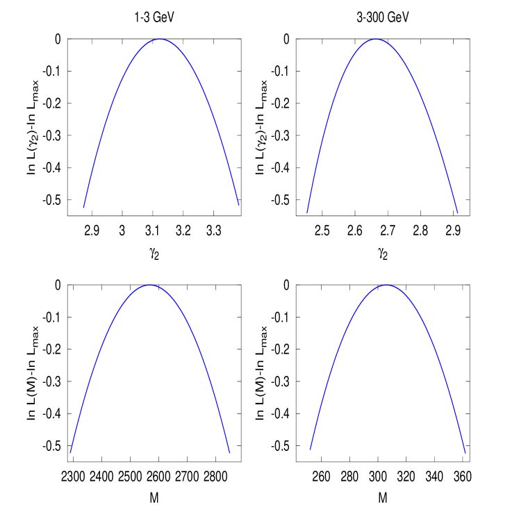
Figure 1: The change of likelihood from its maximum with $\gamma_{2}$ (top) or $M$ (bottom) around their best value when other parameters are fixed on their highest likelihood value. Right and left panels are for 1–3 GeV and 3–300 GeV bands, respectively.

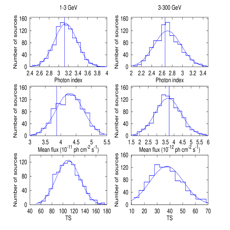
Figure 2: Distributions of photon indexes (top), mean fluxes (middle) and TS (bottom). Right and left panels are for 1–3 GeV and 3–300 GeV bands, respectively. The distribution can be represented by Gaussian functions (dashed line) with central values $\mu$=3.15 (2.71), 4.30 (0.364) $\times 10^{-11}$, 110 (37), respectively, standard deviations $\sigma$=0.23 (0.26), 4.44 (0.755)$\times 10^{-12}$, 21 (13), in the 1–3 (3–300)  GeV. The input photon indexes are 3.12, 2.66, fluxes are 3.87, 0.372 (in unit of [$10^{-11}$ ph cm^-2 s^-1]), respectively, which are indicated by vertical line

References

- Abdo et al. (2009) Abdo A. A., et al., 2009, ApJS, 183, 46
- Abdo et al. (2010a) Abdo A. A., et al., 2010a, ApJ, 715, 429
- Abdo et al. (2010b) Abdo A. A., et al., 2010b, ApJ, 720, 435
- Abdo et al. (2010c) Abdo A. A., et al., 2010c, ApJS, 188, 405
- Abdo et al. (2010d) Abdo A. A., et al., 2010d, Physical Review Letters, 104, 101101
- Ahn er al. (2007) Ahn E. J. er al., 2007, Phys. Rev. D, 76 023517
- Ando & Kusenko (2010) Ando S.& Kusenko A., 2010, ApJ, 2010, 722, L39
- Atwood et al. (2009) Atwood W. B., et al., 2009, ApJ, 697, 1071
- Belikov & Hooper (2010) Belikov A. V. & Hooper D., 2010, Phys. Rev. D, 81, 043505
- Bhattacharya & Sreekumar (2009) Bhattacharya D. & Sreekumar P., 2009, RAA, 9, 509
- Bhattacharya et al. (2009) Bhattacharya D., Sreekumar P. & Mukherjee R., 2009, RAA, 9, 1205
- Cao & Bai (2008) Cao X. W. & Bai J. M., 2008, ApJ, 673, L131
- Cuoco et al. (2010) Cuoco A. et al., 2010, submitted to MNRAS (arXiv:1005.0843)
- Dermer (2007) Dermer C. D., 2007, ApJ, 659, 958
- Fichtel et al. (1975) Fichtel C. E.et al., 1975, ApJ, 198, 163
- Gabici & Blasii, (2003) Gabici S. & Blasi P., 2003, APh, 19, 679
- Ghirlanda et al. (2010a) Ghirlanda G., et al., 2010a, submitted to MNRAS, (arXiv:1003.5163)
- Ghirlanda et al. (2010b) Ghirlanda G., et al., 2010b, submitted to MNRAS, (arXiv:1007.2751)
- Hartman et al. (1999) Hartman R. C., et al. 1999, ApJS, 123, 79
- Inoue & Totani (2009) Inoue Y., & Totani T. 2009,ApJ, 702, 523
- Kneiske & Mannheim (2008) Kneiske T. M. & Mannheim K., 2008, A&A, 479, 41
- Kneiske (2008) Kneiske T.M., 2008, ChJAS, 8, 219
- Mattox et al. (1996) Mattox J. R., et al., 1996, ApJ, 461, 396
- Murphy et al. (2010) Murphy T., at al., 2010, MNRAS, 2010, 402, 2403
- Narumoto & Totani (2006) Narumoto T. & Totani T. 2006, ApJ, 643, 81
- Stecker & Salamon (1996) Stecker F.W. & Salamon M. H. 1996, ApJ, 464, 600
- Thompson et al. (2007) Thompson T. A., Quataert E., & Waxman, E., 2007, ApJ, 654, 219