The contact homology of Legendrian knots with maximal Thurston-Bennequin invariant

Abstract

We show that there exists a Legendrian knot with maximal Thurston-Bennequin invariant whose contact homology is trivial. We also provide another Legendrian knot which has the same knot type and classical invariants but nonvanishing contact homology.

1 Introduction

The Chekanov-Eliashberg invariant [2, 4], which assigns to each Legendrian knot $K$ a differential graded algebra $(Ch(K),\partial)$ over $\mathbb{F}=\mathbb{Z}/2\mathbb{Z}$, has been a powerful tool for classifying Legendrian knots in the standard contact $S^{3}$. The closely related characteristic algebra $\mathcal{C}(K)$ was defined by Ng [12] to be the quotient of $Ch(K)$ by the two-sided ideal $\langle\mathrm{Im}(\partial)\rangle$; if two knots $K$ and $K^{\prime}$ are Legendrian isotopic, then we can add some free generators to $\mathcal{C}(K)$ and $\mathcal{C}(K^{\prime})$ to make them tamely isomorphic. Both of these invariants only provide information about nondestabilizable knots: if $K$ is a stabilized knot, then both the Legendrian contact homology $H_{*}(Ch(K))$ and the characteristic algebra $\mathcal{C}(K)$ vanish. For an introduction to Legendrian knots, see [6].

Shonkwiler and Vela-Vick [17] gave the first examples of Legendrian knots with nonvanishing contact homology which do not have maximal Thurston-Bennequin invariant, representing the knot types $m(10_{161})$ and $m(10_{145})$. Conversely, there are conjecturally nondestabilizable knots of type $m(10_{139})$, $10_{161}$, and $m(12n_{242})$ with non-maximal $tb$ and vanishing contact homology [3, 17]. On the other hand, it is an open question whether there is a Legendrian knot $K$ for which $tb(K)$ is maximal but the contact homology of $K$ vanishes. We will answer this question and show that it is not determined solely by the classical invariants $tb$ and $r$ of $K$:

Theorem.

There are distinct $tb$-maximizing Legendrian representatives $K_{1}$ and $K_{2}$ of $m(10_{132})$ with the same classical invariants such that $K_{1}$ has trivial contact homology, even with $\mathbb{Z}[t,t^{-1}]$ coefficients, while $K_{2}$ does not.

These Legendrian knots, found in Chongchitmate and Ng’s atlas of Legendrian knots [3], can be specified as plat diagrams by the following braid words:

$$K_{1}: 6,7,4,3,7,5,3,6,4,2,5,1,3,2,5,2,4,6,2$$

$$K_{2}: 4,5,3,5,3,2,4,1,3,2,4,2,5,1,3,2,4,4,3,5,4,2$$

Indeed, both knots have classical invariants $tb=-1$ and $r=0$, and Ng [14] showed that $\overline{tb}(m(10_{132}))=-1$ by bounding $\overline{tb}$ for an appropriate cable of $m(10_{132})$. We will prove this theorem in Section 2.

Finally, the proof that $K_{2}$ has nonvanishing contact homology uses an action of $\mathcal{C}(K_{2})$ on an infinite-dimensional vector space, just as the nonvanishing examples in [17] did. In Section 3 we will show that this is necessary in the sense that $\mathcal{C}(K_{2})$ does not have any finite-dimensional representations. It is completely understood when a characteristic algebra $\mathcal{C}$ does not have any $1$-dimensional representations, but we will ask if such a $\mathcal{C}$ can admit maps $\mathcal{C}\to\mathrm{Mat}_{n}(\mathbb{F})$ for some finite $n\geq 2$. We will show that this is possible in general by constructing $2$-dimensional representations for specific Legendrian representatives of negative torus knots.

Acknowledgement.

I would like to thank Ana Caraiani, Tom Mrowka, Lenny Ng, Clayton Shonkwiler, and David Shea Vela-Vick for helpful comments. This work was supported by an NSF Graduate Research Fellowship.

2 The $m(10_{132})$ examples

2.1 The vanishing example

Let $K_{1}$ be the Legendrian representative of $m(10_{132})$ in Figure 1. Its Chekanov-Eliashberg algebra is generated freely over $\mathbb{Z}[t,t^{-1}]$ by elements $x_{1},\dots,x_{23}$ with differentials specified in Appendix A.

Figure 1: The representative $K_{1}$ of $m(10_{132})$, defined by the braid word $6,7,4,3,7,5,3,6,4,2,5,1,3,2,5,2,4,6,2$.

To show that $K_{1}$ has vanishing contact homology, we need to find a relation $\partial x=1$ in $Ch(K_{1})$. Recall that $Ch(K_{1})$ uses a signed Leibniz rule $\partial(vw)=(\partial v)w+(-1)^{|v|}v(\partial w)$, where $|v|$ is the grading of the homogeneous element $v$, and note that the generators with odd grading are

$$x_{2},x_{3},x_{5},x_{9},x_{11},x_{12},x_{13},x_{15},x_{20},x_{21},x_{22},x_{23}.$$

Let $a=x_{12}(x_{4}(1+x_{2}x_{5})-x_{8})+x_{14}x_{5}$ and $b=\partial a$; then $b=x_{10}x_{4}(1+x_{2}x_{5})-x_{10}x_{8}+x_{13}x_{5}$ and $\partial b=0$. Now

$$\partial(x_{22}+x_{12}-ax_{18}) = 1+x_{17}x_{7}+bx_{18}-(bx_{18}+ax_{15}x_{7})$$

$$= 1+(x_{17}-ax_{15})x_{7};$$

let $c=x_{22}+x_{12}-ax_{18}$. Since

$$\partial(x_{17}-ax_{15})=\partial(x_{6}-x_{4}x_{1})=\partial(1+x_{16}x_{19})=0,$$

and $\partial x_{20}=1+(x_{6}-x_{4}x_{1})(1+x_{16}x_{19})$, we can compute

$$\partial\left(x_{20}-c(x_{6}-x_{4}x_{1})(1+x_{16}x_{19})\right)=1-(x_{17}-ax_{15})x_{7}(x_{6}-x_{4}x_{1})(1+x_{16}x_{19}).$$

Finally, we have $-x_{7}(x_{6}-x_{4}x_{1})=\partial(x_{9}+x_{2})$, so we conclude that

$$\partial\left(x_{20}-\left(c(x_{6}-x_{4}x_{1})+(x_{17}-ax_{15})(x_{9}+x_{2})\right)(1+x_{16}x_{19})\right)=1,$$

and so $K_{1}$ has trivial contact homology over $\mathbb{Z}[t,t^{-1}]$ as desired.

2.2 The nonvanishing example

Let $K_{2}$ be the Legendrian representative of $m(10_{132})$ in Figure 2. The algebra $Ch(K_{2})$ is generated freely over $\mathbb{F}=\mathbb{Z}/2\mathbb{Z}$ by $x_{1},\dots,x_{25}$ with differentials specified in Appendix B. In order to show that $K_{2}$ has nontrivial contact homology, it will suffice to show that the characteristic algebra $\mathcal{C}_{2}=\mathcal{C}(K_{2})$ is nonvanishing [17].

Figure 2: The representative $K_{2}$ of $m(10_{132})$, defined by the braid word $4,5,3,5,3,2,4,1,3,2,4,2,5,1,3,2,4,4,3,5,4,2$.

The differential in $\mathcal{C}_{2}$ immediately gives us $x_{1}=x_{6}=0$, and

$$x_{12}=\partial(x_{12}x_{23}+x_{15}x_{22}+x_{17}x_{18})$$

gives $x_{12}=0$, hence $\partial x_{24}=0$ becomes $(1+x_{5}(x_{2}+x_{3}))x_{20}=1$. Then we can use $(\partial x_{13})x_{20}=0$ and $(\partial x_{17})x_{20}=0$ to get $x_{11}=0$ and $x_{15}=0$, so

$$x_{1}=x_{6}=x_{11}=x_{12}=x_{15}=0.$$

Furthermore, $\partial x_{21}=0$ becomes $x_{14}=cx_{20}$, so $\partial x_{25}=0$ gives us $x_{14}=x_{20}$.

Consider the quotient of $\mathcal{C}_{2}$ by the two-sided ideal

$$\mathcal{I}=\langle x_{3},x_{7},x_{8},x_{9},x_{10},x_{13}+1+x_{2}x_{5},x_{17},x_{19},x_{21},\dots,x_{25}\rangle.$$

The quotient $\mathcal{C}_{2}/\mathcal{I}$ is generated by $x_{2},x_{4},x_{5},x_{14},x_{16},x_{18}$, and its nontrivial relations are $c=x_{2}+x_{14}(1+x_{2}x_{5})+x_{16}(1+x_{5}x_{2})=1$ and

$$x_{4} = x_{5}(1+x_{2}x_{4})$$

$$x_{18} = 1+x_{2}x_{4}$$

$$0 = (1+x_{5}x_{2})x_{18}$$

$$1 = (1+x_{2}x_{5})x_{18}$$

$$1 = (1+x_{5}x_{2})x_{14}.$$

Note that the pair of relations $x_{4}=x_{5}(1+x_{2}x_{4})$ and $x_{18}=1+x_{2}x_{4}$ are equivalent to $x_{4}=x_{5}x_{18}$ and $(1+x_{2}x_{5})x_{18}=1$, the latter of which is already known, so we can replace the pair with $x_{4}=x_{5}x_{18}$. Furthermore, multiplying the $c=1$ equation on the right by $x_{18}$ gives $x_{14}=(1+x_{2})x_{18}$, hence the last relation becomes $(1+x_{5}x_{2})x_{2}x_{18}=1$. Then the $c=1$ equation becomes

$$x_{16}(1+x_{5}x_{2})=(1+x_{2})(1+x_{18}(1+x_{2}x_{5}))$$

so we multiply on the right by $x_{2}x_{18}$ and get

$$x_{16}=(1+x_{2})(x_{2}x_{18}+x_{18}x_{2}(1+x_{5}x_{2})x_{18})=(1+x_{2})x_{2}x_{18}.$$

Thus we see that $x_{4}$, $x_{14}$, and $x_{16}$ can be expressed in terms of $x_{2}$, $x_{5}$, and $x_{18}$, and $c=1$ can be rewritten as

$$0=(1+x_{2})\left(1+x_{18}(1+x_{2}x_{5})+x_{2}x_{18}(1+x_{5}x_{2})\right).$$

Relabeling $x_{2},x_{5},x_{18}$ as $a,b,c$ respectively, we have a homomorphism from $\mathcal{C}_{2}/\mathcal{I}$ to the quotient $R$ of the free algebra $\mathbb{F}\langle a,b,c\rangle$ by the two-sided ideal generated by the relations

$$0 = 1+c(1+ab)+ac(1+ba)$$

$$0 = (1+ba)c$$

$$1 = (1+ab)c$$

$$1 = (1+ba)ac.$$

Proposition 2.1.

The algebra $R$ is nontrivial.

Proof.

We will construct an infinite-dimensional representation of $R$, following ideas from [17]. Let $\mathcal{H}$ be a countable-dimensional $\mathbb{F}$-vector space, with basis $\{v_{0},v_{1},v_{2},\dots\}$, and write $\mathcal{H}=\mathcal{H}_{1}\oplus\mathcal{H}_{2}$ where each $\mathcal{H}_{i}$ summand is isomorphic to $\mathcal{H}$. Let $f,g:\mathcal{H}\to\mathcal{H}$ be homomorphisms defined by $f(v_{i})=v_{2i}$ and $g(v_{i})=v_{2i+1}$, so that the diagrams

represent isomorphisms $\mathcal{H}\stackrel{{\scriptstyle\sim}}{{\to}}\mathcal{H}_{1}$ and $\mathcal{H}\stackrel{{\scriptstyle\sim}}{{\to}}\mathcal{H}_{2}$, respectively. We also define homomorphisms $p,s:\mathcal{H}\to\mathcal{H}$ by $p(v_{i})=v_{i-1}$ for $i\geq 1$, $p(v_{0})=0$ and $s(v_{i})=v_{i+1}+v_{2(i+1)}$. It is straightforward to check the identities

$$s\circ p=f+1, p\circ g=f, p\circ s=g+1.$$

We define a right action of $a$ and $b$ on $\mathcal{H}\cong\mathcal{H}_{1}\oplus\mathcal{H}_{2}$ by the diagrams

respectively. Then we can compute the action of $ab$ and $ba$ by concatenating the $a$ and $b$ diagrams to get

respectively, hence by the above identities $1+ab$ and $1+ba$ are exactly the specified isomorphisms $\mathcal{H}\stackrel{{\scriptstyle\sim}}{{\to}}\mathcal{H}_{1}$ and $\mathcal{H}\stackrel{{\scriptstyle\sim}}{{\to}}\mathcal{H}_{2}$. Finally, let $c$ act on $\mathcal{H}$ as the map

where the indicated isomorphism is the inverse of $\mathcal{H}\stackrel{{\scriptstyle\sim}}{{\to}}\mathcal{H}_{1}$. Then the composition $ac$ is the homomorphism

where the isomorphism is inverse to $\mathcal{H}\stackrel{{\scriptstyle\sim}}{{\to}}\mathcal{H}_{2}$. It is now easy to check that $(1+ab)c=1$, $(1+ba)c=0$, and $(1+ba)ac=1$. Finally, we note that $c(1+ab)$ is the projection of $\mathcal{H}$ onto $\mathcal{H}_{1}\subset\mathcal{H}$ and likewise $ac(1+ba)$ is the projection onto $\mathcal{H}_{2}$, hence

$$1=c(1+ab)+ac(1+ba).$$

Therefore the action which we have constructed satisfies all of the defining relations of $R$. ∎

Since $R$ is nonvanishing and we have a homomorphism $\mathcal{C}_{2}\to\mathcal{C}_{2}/\mathcal{I}\to R$, we conclude that $\mathcal{C}_{2}$ (and hence the contact homology of $K_{2}$) is nonvanishing as well.

3 Finite-dimensional representations of $\mathcal{C}(K)$

Although the Legendrian knot $K_{2}$ of Section 2.2 is now known to have nontrivial contact homology and characteristic algebra, one can ask for a simpler proof of this fact; in particular, one can ask if $\mathcal{C}_{2}$ has any finite-dimensional representations. The answer in this case is no.

Lemma 3.1.

Suppose that an $\mathbb{F}$-algebra $\mathcal{A}$ has a relation of the form $ab=1$. If the quotient of $\mathcal{A}$ by the two-sided ideal $\langle ba-1\rangle$ is trivial, i.e. if $0=1$ in $\mathcal{A}/\langle ba-1\rangle$, then there is no representation $\mathcal{A}\to\mathrm{Mat}_{n}(\mathbb{F})$ for any $n$.

Proof.

Suppose there is a homomorphism $\varphi:\mathcal{A}\to\mathrm{Mat}_{n}(\mathbb{F})$, so in particular $\varphi(1)=1$. The equation $\varphi(ab-1)=0$ implies that $\varphi(a)$ and $\varphi(b)$ are inverse matrices, so they commute and $\varphi(ba-1)=0$ as well. Then $\varphi$ factors through the quotient $\mathcal{A}/\langle ba-1\rangle$ in which $0=1$, hence $\varphi(1)=\varphi(0)=0$, which is a contradiction. ∎

Now in $\mathcal{C}_{2}$, we showed in Section 2.2 that $x_{11}=x_{12}=0$ and $(1+x_{5}(x_{2}+x_{3}))x_{20}=1$. If we impose the relation $x_{20}(1+x_{5}(x_{2}+x_{3}))=1$, then $x_{18}=x_{20}(\partial x_{22})=0$ as well and so $0=\partial x_{23}=1$, hence $\mathcal{C}_{2}$ has no finite-dimensional representations by Lemma 3.1.

Lemma 3.1 can also be used to prove that the characteristic algebra of the Legendrian $m(10_{161})$ studied in [17] has no finite-dimensional representations, by adding $x_{28}x_{13}=1$ to the relations $\partial x_{i}=0$ in [17, Appendix A] and showing that $0=1$ as a consequence, and similarly for the $m(10_{145})$ representative mentioned in the same article. Neither one of these knots has maximal Thurston-Bennequin invariant.

On the other hand, it is interesting to ask when the characteristic algebra $\mathcal{C}$ of a Legendrian knot $K$ has $n$-dimensional representations. For $n=1$ the answer depends only on $tb$ and the topological knot type:

Proposition 3.2.

There is a homomorphism $\mathcal{C}\to\mathrm{Mat}_{1}(\mathbb{F})\cong\mathbb{F}$ if and only if the Kauffman bound

$$tb(K)\leq\textrm{\emph{min-deg}}_{a}F_{K}(a,x)-1$$

(see [10]) is sharp.

Proof.

The Kauffman bound for $K$ is achieved if and only if a front diagram for $K$ admits an ungraded normal ruling [15], which happens if and only if $Ch(K)$ admits an ungraded augmentation [8, 9, 16]. An augmentation is an algebra homomorphism $Ch(K)\stackrel{{\scriptstyle\epsilon}}{{\to}}\mathbb{F}$ which satisfies $\epsilon\circ\partial=0$, and these correspond bijectively to algebra homomorphisms $\mathcal{C}\to\mathbb{F}$, so the latter exists if and only if the Kauffman bound is sharp. ∎

In particular, the Kauffman bound is known to be sharp for all knots with at most 9 crossings except for $m(8_{19})$ and $m(9_{42})$ (see [13]); for all 10-crossing knots except $m(10_{124})$, $m(10_{128})$, $m(10_{132})$, and $m(10_{136})$ [1]; and for all alternating knots [15]. Thus the characteristic algebra of a Legendrian representative of one of these knot types has a 1-dimensional representation if and only if it is $tb$-maximizing.

We will now demonstrate the existence of infinitely many Legendrian knots whose characteristic algebras have $n$-dimensional representations for $n=2$ but not for $n=1$. For convenience, we will use the following presentation of $\mathrm{Mat}_{2}(\mathbb{F})$.

Lemma 3.3.

The ring $\mathrm{Mat}_{2}(\mathbb{F})$ has a presentation of the form

$$\frac{\mathbb{F}\langle a,b\rangle}{\langle a^{2}=b^{2}=0,ab+ba=1\rangle}.$$

Proof.

Let $R$ be the $\mathbb{F}$-algebra with the given presentation, and consider a map $\varphi:R\to\mathrm{Mat}_{2}(\mathbb{F})$ of the form

$$a \mapsto A=\left(\begin{array}[]{cc}0&1\\ 0&0\end{array}\right)$$

$$b \mapsto B=\left(\begin{array}[]{cc}0&0\\ 1&0\end{array}\right).$$

It is easy to check that $A^{2}=B^{2}=0$ and $AB+BA=I$, so $\varphi$ is a valid homomorphism, and since $A,B,AB,BA$ form an additive basis of $\mathrm{Mat}_{2}(\mathbb{F})$ it is surjective. To check that $\varphi$ is also injective, we note that any nonzero monomial in $R$ is equal to one of $1,a,b,ab,$ or $ba=1+ab$, and so $1,a,b,ab$ span $R$ as an $\mathbb{F}$-vector space; since the image of $\varphi$ has order $|\mathrm{Mat}_{2}(\mathbb{F})|=16\geq|R|$ it follows that $\varphi$ is injective. ∎

Let $T_{p,-q}$ be the Legendrian representative of the $(p,-q)$-torus knot as in Figure 3, where $q>p\geq 3$; there are $p$ numbered left cusps at the leftmost edge of the diagram, $q-p$ left cusps in the innermost region of the diagram, and $q$ right cusps. The algebra $Ch(T_{p,-q})$ can be computed following [12]: the front projection is simple, so $Ch(T_{p,-q})$ is generated by crossings and right cusps and the differential counts admissible embedded disks in the diagram.

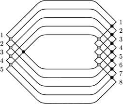
Figure 3: A Legendrian representative $T_{5,-8}$ of the $(5,-8)$-torus knot.

We label the generators of $Ch(T_{p,-q})$ as follows. On the left half of the diagram, $x_{ij}$ is the intersection of the strands through the numbered left cusps $i$ and $j$ for $1\leq i<j\leq p$. On the right half, $y_{ij}$ denotes the intersection of strands through the numbered right cusps $i$ and $j$ for $1\leq i<j\leq\max(q,i+p-1)$, and $z_{i}$ is the $i$th right cusp.

We define an algebra homomorphism $f:Ch(T_{p,-q})\to\mathrm{Mat}_{2}(\mathbb{F})$ by sending all generators to $0$ except

$$x_{i,i+1},y_{j,j+p-1} \mapsto a$$

$$x_{1,p},y_{j,j+1} \mapsto b.$$

In Figure 3, $f$ is equal to $a$ on the crossings marked with gray dots, $b$ on the crossings marked with black dots, and $0$ on all other crossings and right cusps. If we can show that $f(\partial v)=0$ for all generators $v$, then $f$ is a morphism of DGAs (where $\mathrm{Mat}_{2}(\mathbb{F})$ has trivial differential) and it induces a representation $\mathcal{C}(T_{p,-q})\to\mathrm{Mat}_{2}(\mathbb{F})$.

Proposition 3.4.

The homomorphism $f:Ch(T_{p,-q})\to\mathrm{Mat}_{2}(\mathbb{F})$ satisfies $f(\partial v)=0$ for all $v$.

Proof.

Call an admissible disk nontrivial if none of its corners are in $\ker(f)$. Then it is easy to see that any nontrivial disk has exactly two corners, and if both corners have the same color (in the sense of Figure 3, i.e. if they are sent to the same element of $\mathrm{Mat}_{2}(\mathbb{F})$) then the contribution of this disk to $f(\partial v)$ is either $a^{2}=0$ or $b^{2}=0$. Thus we can determine $f(\partial v)$ by only counting disks with initial vertex at $v$ and having exactly one gray corner and one black corner.

If $v$ is the right cusp $z_{i}$, then there are two nontrivial disks contributing $ab$ and $ba$ to the differential, so $f(\partial z_{i})=1+ab+ba=0$. For all crossings $v$, however, the only possible black corner for a nontrivial disk is $x_{1,p}$. Such a disk must include either the first or the $p$th numbered left cusp on its boundary depending on whether the interior of the disk is immediately above or below $x_{1,p}$, but then the boundary of the disk must pass through either $z_{1}$ or $z_{q}$, which in particular is to the right of $v$, and so it cannot contribute to $f(\partial v)$. We conclude that $f(\partial v)=0$ for all generators $v$ of $Ch(T_{p,-q})$, as desired. ∎

We can compute $tb(T_{p,-q})=-pq$ for all $p$ and $q$, hence $T_{p,-q}$ is $tb$-maximizing by the classification of Legendrian torus knots [7], but for odd $p$ the Kauffman bound is $tb(K)\leq-pq+q-p$ [5]. Using Proposition 3.2, we conclude:

Corollary 3.5.

Let $p\geq 3$ be odd and $q>p$. Then the characteristic algebra $\mathcal{C}(T_{p,-q})$ admits an $n$-dimensional representation for $n=2$ but not for $n=1$.

Remark 3.6.

The knots $T_{3,-4}$ and $T_{3,-5}$ are the unique $tb$-maximizing representatives of $m(8_{19})$ and $m(10_{124})$ up to change of orientation [7], so if any $tb$-maximizing Legendrian representative of a knot with at most 10 crossings has vanishing contact homology or characteristic algebra (such as the $m(10_{132})$ of Section 2.1) then it must represent one of $m(9_{42})$, $m(10_{128})$, $m(10_{132})$, or $m(10_{136})$. The characteristic algebra of the known $tb$-maximizing Legendrian $m(9_{42})$, which has a plat diagram with braid word

$$2,1,1,4,5,3,5,3,2,4,3,3,2,4,$$

can also be shown to have a $2$-dimensional representation, so it does not vanish.

It is not known whether there are Legendrian knots whose characteristic algebras have representations of minimal dimension $n\geq 3$, or whether this minimal dimension can be used to distingush any Legendrian knots with nontrivial characteristic algebras and the same classical invariants. We leave open the question of which Legendrian knots $K$ admit representations $\mathcal{C}(K)\to\mathrm{Mat}_{n}(\mathbb{F})$ for fixed $n\geq 2$ or even for any finite $n$.

Appendix A The differential of the vanishing $m(10_{132})$

Let $K_{1}$ be the representative of $m(10_{132})$ with braid word

$$6,7,4,3,7,5,3,6,4,2,5,1,3,2,5,2,4,6,2.$$

Then $Ch(K_{1})$ has generators $x_{1},\dots,x_{23}$ over $\mathbb{Z}[t,t^{-1}]$ with the following nonzero differentials [11]:

$$\partial x_{2} = -x_{1}$$

$$\partial x_{4} = x_{3}$$

$$\partial x_{6} = x_{3}x_{1}$$

$$\partial x_{8} = x_{3}+x_{3}x_{2}x_{5}-x_{6}x_{5}$$

$$\partial x_{9} = x_{1}+x_{7}x_{4}x_{1}-x_{7}x_{6}$$

$$\partial x_{11} = 1+x_{2}x_{5}+x_{7}x_{4}+x_{7}x_{4}x_{2}x_{5}-x_{7}x_{8}+x_{9}x_{5}$$

$$\partial x_{12} = x_{10}$$

$$\partial x_{13} = x_{10}x_{4}x_{1}-x_{10}x_{6}$$

$$\partial x_{14} = -x_{12}x_{4}x_{1}+x_{12}x_{6}+x_{13}$$

$$\partial x_{17} = x_{10}x_{4}x_{15}+x_{10}x_{4}x_{2}x_{5}x_{15}-x_{10}x_{8}x_{15}+x_{13}x_{5}x_{15}$$

$$\partial x_{18} = -x_{15}x_{7}$$

$$\partial x_{20} = 1-x_{4}x_{1}+x_{6}-x_{4}x_{1}x_{16}x_{19}+x_{6}x_{16}x_{19}$$

$$\partial x_{21} = 1-x_{12}x_{4}x_{15}-x_{12}x_{4}x_{2}x_{5}x_{15}+x_{12}x_{8}x_{15}-x_{14}x_{5}x_{15}+x_{17}$$

$$-x_{19}x_{5}x_{15}-x_{19}x_{16}x_{12}x_{4}x_{15}-x_{19}x_{16}x_{12}x_{4}x_{2}x_{5}x_{15}$$

$$+x_{19}x_{16}x_{12}x_{8}x_{15}-x_{19}x_{16}x_{14}x_{5}x_{15}+x_{19}x_{16}x_{17}$$

$$\partial x_{22} = 1-x_{10}+x_{17}x_{7}+x_{10}x_{4}x_{18}+x_{10}x_{4}x_{2}x_{5}x_{18}-x_{10}x_{8}x_{18}+x_{13}x_{5}x_{18}$$

$$\partial x_{23} = t^{-1}+x_{15}x_{2}+x_{15}x_{7}x_{4}x_{2}+x_{15}x_{9}-x_{18}x_{3}x_{2}+x_{18}x_{6}.$$

Appendix B The differential of the nonvanishing $m(10_{132})$

Let $K_{2}$ be the representative of $m(10_{132})$ with braid word

$$4,5,3,5,3,2,4,1,3,2,4,2,5,1,3,2,4,4,3,5,4,2.$$

Then $Ch(K_{2})$ has generators $x_{1},\dots,x_{25}$ over $\mathbb{Z}/2\mathbb{Z}$ with the following nonzero differentials [11]:

$$\partial x_{2}=\partial x_{3} = x_{1}$$

$$\partial x_{7} = x_{4}+x_{5}(1+(x_{2}+x_{3})x_{4})$$

$$\partial x_{8} = x_{6}$$

$$\partial x_{9} = x_{6}(1+(x_{2}+x_{3})x_{4})$$

$$\partial x_{10} = x_{9}+x_{8}(1+(x_{2}+x_{3})x_{4})$$

$$\partial x_{13} = x_{6}(x_{2}+x_{3})+x_{11}(1+x_{5}(x_{2}+x_{3}))$$

$$\partial x_{14} = (1+(x_{2}+x_{3})x_{4})x_{12}$$

$$\partial x_{15} = x_{12}x_{11}$$

$$\partial x_{16} = x_{14}x_{11}+(1+(x_{2}+x_{3})x_{4})x_{15}$$

$$\partial x_{17} = x_{12}(x_{13}+x_{8}(x_{2}+x_{3}))+x_{15}(1+x_{5}(x_{2}+x_{3}))$$

$$\partial x_{19} = (1+(x_{2}+x_{3})x_{4})+cx_{18}$$

$$\partial x_{20} = x_{18}x_{12}$$

$$\partial x_{21} = x_{14}+x_{19}x_{12}+cx_{20}$$

$$\partial x_{22} = (1+x_{5}(x_{2}+x_{3}))x_{18}$$

$$\partial x_{23} = 1+x_{11}x_{22}+(x_{13}+x_{8}(x_{2}+x_{3}))x_{18}$$

$$\partial x_{24} = 1+x_{22}x_{12}+(1+x_{5}(x_{2}+x_{3}))x_{20}$$

$$\partial x_{25} = 1+c$$

where

$$c=x_{2}+x_{3}+(1+(x_{2}+x_{3})x_{4})x_{17}+x_{14}(x_{13}+x_{8}(x_{2}+x_{3}))+x_{16}(1+x_{5}(x_{2}+x_{3})).$$

References

• [1] J. C. Cha and C. Livingston, KnotInfo: Table of Knot Invariants, http://www.indiana.edu/~knotinfo, December 3, 2010.
• [2] Yuri Chekanov, Differential algebra of Legendrian links, Invent. Math. 150 (2002), no. 3, 441–483.
• [3] Wutichai Chongchitmate and Lenhard Ng, An atlas of Legendrian knots, arXiv:1010.3997.
• [4] Yakov Eliashberg, Invariants in contact topology, Proceedings of the International Congress of Mathematicians, Vol. II (Berlin, 1998), Doc. Math. 1998, Extra Vol. II, 327–338 (electronic).
• [5] Judith Epstein and Dmitry Fuchs, On the invariants of Legendrian mirror torus links, Symplectic and contact topology: interactions and perspectives (Toronto, ON/Montreal, QC, 2001), 103–115, Fields Inst. Commun., 35, Amer. Math. Soc., Providence, RI, 2003.
• [6] John Etnyre, Legendrian and transversal knots, Handbook of knot theory, 105–185, Elsevier B. V., Amsterdam, 2005.
• [7] John Etnyre and Ko Honda, Knots and contact geometry. I. Torus knots and the figure eight knot, J. Symplectic Geom. 1 (2001), no. 1, 63–120.
• [8] Dmitry Fuchs, Chekanov-Eliashberg invariant of Legendrian knots: existence of augmentations, J. Geom. Phys. 47 (2003), no. 1, 43–65.
• [9] Dmitry Fuchs and Tigran Ishkhanov, Invariants of Legendrian knots and decompositions of front diagrams, Mosc. Math. J. 4 (2004), no. 3, 707–717.
• [10] Dmitry Fuchs and Serge Tabachnikov, Invariants of Legendrian and transverse knots in the standard contact space, Topology 36 (1997), no. 5, 1025–1053.
• [11] P. Melvin et al., Legendrian Invariants.nb, Mathematica program available at http://www.haverford.edu/math/jsabloff/Josh_Sabloff/Research.html.
• [12] Lenhard Ng, Computable Legendrian invariants, Topology 42 (2003), no. 1, 55–82.
• [13] Lenhard Ng, Maximal Thurston-Bennequin number of two-bridge links, Algebr. Geom. Topol. 1 (2001), 427–434 (electronic).
• [14] Lenhard Ng, On arc index and maximal Thurston-Bennequin number, arXiv:math.GT/0612356.
• [15] Dan Rutherford, Thurston-Bennequin number, Kauffman polynomial, and ruling invariants of a Legendrian link: the Fuchs conjecture and beyond, Int. Math. Res. Not. 2006, Art. ID 78591, 15 pp.
• [16] Joshua Sabloff, Augmentations and rulings of Legendrian knots, Int. Math. Res. Not. 2005, no. 19, 1157–1180.
• [17] Clayton Shonkwiler and David Shea Vela-Vick, Legendrian contact homology and nondestabilizability, J. Symplectic Geom. 9 (2011), no. 1, 1–12.