Dynamics of open quantum systems with initial system-reservoir correlations

Abstract

In this paper, the exact dynamics of open quantum systems in the presence of initial system-reservoir correlations is investigated for a photonic cavity system coupled to a general non-Markovian reservoir. The exact time-convolutionless master equation incorporating with initial system-reservoir correlations is obtained. The non-Markovian dynamics of the reservoir and the effects of the initial correlations are embedded into the time-dependent coefficients in the master equation. We show that the effects induced by the initial correlations play an important role in the non-Markovian dynamics of the cavity but they are washed out in the steady-state limit in the Markovian regime. Moreover, the initial two-photon correlation between the cavity and the reservoir can induce nontrivial squeezing dynamics to the cavity field.

I Introduction

The study of dynamics of open quantum systems continuously receives attentions because of its fundamental importance in quantum physics and also because of the rapid development of quantum technologies. Previous studies on the dynamics of open quantum systems mainly lie on the Lindblad-type master equation bm1 ; bm2 ; bm3 , where the characteristic time of the environment is sufficiently shorter than that of the system such that the non-Markovian memory effect is negligible, and so does for initial system-reservoir correlations. However, the new development in ultrafast photonics, ultracold atomic physics, nanoscience and technology as well as quantum information science strongly suggests that the non-Markovian dynamics in ultrafast and ultrasmall open systems should play an important role, and the associated effects (including the initial system-reservoir correlations) should be fully taken into account. To this end, the more rigorous approach is demanded for the study of non-Markovian dynamics of open quantum systems incorporating with the initial system-reservoir correlations.

The exact description of open quantum systems has indeed been explored extensively in the literature, mainly focusing on quantum Brown motion based on Feynman-Vernon influence functional Fey63118 ; Cal83587 ; Haa852462 ; Hu922843 ; Hal962012 ; Food01105020 and stochastic diffusion Schrödinger equation Str981699 ; Str994909 ; Yu04062107 . Extending the Feynman-Vernon influence functional to other open quantum systems has also achieved a great success recently, including the exact master equation for electron systems and the nonequilibrium quantum transport theory in various nanostructures Tu08235311 ; Tu09631 ; Jin10083013 and the exact master equation for micro- or nanocavities in photonic crystals and the quantum transport theory for photonic crystals Xio10012105 ; Wu1018407 ; Lei104570 . However, in most of these investigations, the system and the reservoir are often assumed to be initially uncorrelated with each other Leg871 . Realistically, it is possible and often unavoidable in experiments that the system and its environment are correlated closely at the beginning, especially for the cases of the system strongly coupled to the reservoir ee . Various initial-correlation induced effects have been investigated in different open quantum systems src0 ; src1 ; src2 ; src3 ; src4 ; src5 ; src7 ; src8 ; src6 ; src9 ; src10 . For example, it has been recently shown that the initial correlations between a qubit and its environment can lead to the distance growth of two quantum states over its initial value src7 ; src8 . It has also been demonstrated that the initial correlations have nontrivial differences in quantum tomography process src6 . Besides, it has been found that the initial system-reservoir correlations have significant effects on the entanglement in a two-qubit system src9 ; src10 .

In this paper, the dynamics of open quantum systems in the presence of initial system-reservoir correlations is investigated with a photonic cavity system coupled to a non-Markovian reservoir as a specific example. By solving the exact dynamics of the cavity system, the effects of the initial correlations are explicitly built into the equations of motion for the intensity and the two-photon correlation function of the cavity field. We then obtain the exact master equation incorporating with the initial correlations which induce new terms and also modify the time-dependent dissipation and fluctuation coefficients in the master equation. Taking a nanocavity coupled to a coupled resonator optical waveguide (serving as a structured reservoir) as an experimentally realizable system, we find that the effects of the initial correlations are fragile for a Markovian reservoir but play an important role in the non-Markovian regime. In fact, in the strong non-Markovian regime, the initial two-photon correlation between the cavity and the reservoir can induce oscillating squeezing dynamics in the cavity. But in the Markovian regime, the initial correlations will be washed out in the steady-state limit.

The rest of the paper is organized as follows. In Sec. II, the dynamics of open quantum systems with initial system-reservoir correlations is formulated for a photonic cavity system coupled to a general non-Markovian reservoir. In Sec. III, we construct the exact time-convolutionless master equation incorporating with the initial correlations, where the effects from the initial correlations are explicitly embedded into the time-dependent coefficients in the master equation. In Sec. IV, an experimentally realizable example is considered to analytically and numerically examine the influence of the initial correlations on the dynamics of open quantum systems. At last, a summary is given in Sec. V.

II Non-Markovian dynamics with initial system-reservoir correlations

To be specific, we consider here a single-mode photonic cavity system coupled to a general non-Markovian reservoir, where the single-mode cavity system could be a nanocavity in nanostructures or photonic crystals, and the non-Markovian environment may be a structured photonic reservoir stru-reservoir . The Hamiltonian of the system can be expressed as a Fano-type model of a localized state coupled with a continuum Fano611866 :

$$H=\omega_{c}a^{\dagger}a+\sum_{k}\omega_{k}b_{k}^{\dagger}b_{k}\ +\sum_{k}V_{k}(ab_{k}^{\dagger}+b_{k}a^{\dagger}),$$ (1)

where the first term is the Hamiltonian of the cavity field with frequency $\omega_{c}$, and $a^{\dagger}$ and $a$ are the creation and annihilation operators of the cavity field; the second term describes a general non-Markovian reservoir which is modeled as a collection of infinite photonic modes, where $b_{k}^{\dagger}$ and $b_{k}$ are the corresponding creation and annihilation operators of the $k$-th photonic mode with frequency $\omega_{k}$. The third term characterizes the system-reservoir coupling with the coupling strength $V_{k}$ between the cavity field and the $k$-th photonic mode. For convenience, we take $\hbar=1$ throughout the paper.

We shall use the equation of motion approach to solve the dynamics of the cavity system and the reservoir, from which the general initial correlations between the cavity and the reservoir can be fully taken into account. The time evolution of the cavity field operator $a(t)=e^{iHt}ae^{-iHt}$ and the reservoir field operators $b_{k}(t)=e^{iHt}b_{k}e^{-iHt}$ in the Heisenberg picture obey the equations of motion

$$\frac{d}{dt}a(t)=-i[a(t),H]=-i\omega_{c}a(t)-i\sum_{k}V_{k}b_{k}(t),$$ (2a)

$$\frac{d}{dt}b_{k}(t)=-i[b_{k}(t),H]=-i\omega_{k}b_{k}(t)-iV_{k}a(t).$$ (2b)

Solving Eq. (2b) for $b_{k}(t)$

$$b_{k}(t)=b_{k}(0)e^{-i\omega_{k}t}-iV_{k}\int_{0}^{t}d\tau a(\tau)e^{-i\omega_{k}(t-\tau)},$$ (3)

we obtain

$$\frac{d}{dt}a(t)=-i\omega_{c}a(t)-\int_{0}^{t}d\tau g(t-\tau)a(\tau)$$

$$-i\sum_{k}V_{k}b_{k}(0)e^{-i\omega_{k}t}.$$ (4)

Here, the memory kernel $g(\tau)=\sum_{k}|V_{k}|^{2}e^{-i\omega_{k}\tau}$ characterizes the non-Markovian dynamics of the reservoir. For a continuous reservoir spectrum, we have $g(\tau)=\int_{0}^{\infty}\frac{d\omega}{2\pi}J(\omega)e^{-i\omega\tau}$, where $J(\omega)=2\pi\varrho(\omega)|V(\omega)|^{2}$ is the spectral density of the reservoir, with $\varrho(\omega)$ being the density of states and $V(\omega)$ the coupling between the cavity and the reservoir in the frequency domain.

Because of the linearity of Eq.(4), the cavity field operator $a(t)$ can be expressed, in terms of the initial field operators $a(0)$ and $b_{k}(0)$ of the cavity and the reservoir, as

$$a(t)=u(t)a(0)+f(t),$$ (5)

where the time-dependent coefficient $u(t)$ and $f(t)$ are determined from Eq.(4) and given by

$$\frac{d}{dt}u(t)=-i\omega_{c}u(t)-\int_{0}^{t}d\tau g(t-\tau)u(\tau),$$ (6a)

$$\frac{d}{dt}f(t)=-i\omega_{c}f(t)-\int_{0}^{t}d\tau g(t-\tau)f(\tau)$$

$$-i\sum_{k}V_{k}b_{k}(0)e^{-i\omega_{k}\tau},$$ (6b)

subjected to the initial conditions $u(0)=1$ and $f(0)=0$. The integrodifferential equation (6a) shows that $u(t)$ is just the propagating function of the cavity field (the retarded Green function in nonequilibrium Green function theory green ). In addition, $f(t)$ is in fact an operator coefficient and its solution can be obtained analytically from the inhomogeneous equation of Eq. (6):

$$f(t)=-i\sum_{k}V_{k}b_{k}(0)\int_{0}^{t}d\tau e^{-i\omega_{k}\tau}u(t-\tau).$$ (7)

From Eqs. (5)-(7) we can determine the exact non-Markovian dynamics of the cavity field coupled to a general reservoir with arbitrary initial system-reservoir correlations, upon a given initial state $\rho_{\rm tot}(0)$ of the whole system. In the Heisenberg picture, quantum states are time-independent. Once $\rho_{\rm tot}(0)=\rho_{\rm tot}$ is given, the time evolution of any physical observable can be obtained directly from Eqs. (5)-(7) through the relation

$$\langle f(a^{\dagger}(t),a(t))\rangle={\rm tr}[f(a^{\dagger}(t),a(t))\rho_{\rm tot}].$$ (8)

For example, the time evolution of the expectation values $\langle a(t)\rangle$, $n(t)\equiv\langle a^{\dagger}(t)a(t)\rangle$, and $s(t)\equiv\langle a(t)a(t)\rangle$, which respectively describe the cavity amplitude, the cavity intensity, and the two-photon correlation of the cavity field, can be expressed explicitly by the following solution

$$\langle a(t)\rangle=u(t)\langle a(0)\rangle+\upsilon_{0}(t),$$ (9a)

$$n(t)=|u(t)|^{2}n(0)+2{\rm Re}[u^{*}(t)\nu_{1}(t)]+\upsilon_{1}(t),$$ (9b)

$$s(t)=u^{2}(t)s(0)+2u(t)\nu_{2}(t)+\upsilon_{2}(t),$$ (9c)

where $\langle a(0)\rangle,n(0)$ and $s(0)$ are the corresponding initial conditions. Other time-dependent functions in Eq. (9) are given by

$$\nu_{1}(t) =\langle a^{\dagger}(0)f(t)\rangle=-i\int_{0}^{t}\sum_{k}V_{k}\langle a^{\dagger}(0)b_{k}(0)\rangle e^{-i\omega_{k}\tau}u(t-\tau)d\tau,$$ (10a)

$$\nu_{2}(t) =\langle a(0)f(t)\rangle=-i\int_{0}^{t}\sum_{k}V_{k}\langle a(0)b_{k}(0)\rangle e^{-i\omega_{k}\tau}u(t-\tau)d\tau,$$ (10b)

$$\upsilon_{0}(t) =-i\int_{0}^{t}\sum_{k}V_{k}\langle b_{k}(0)\rangle e^{-i\omega_{k}\tau}u(t-\tau)d\tau,$$ (10c)

$$\upsilon_{1}(t) =\langle f^{\dagger}(t)f(t)\rangle=\int_{0}^{t}d\tau\int_{0}^{t}d\tau^{\prime}\sum_{kk^{\prime}}V^{*}_{k}V_{k^{\prime}}\langle b^{\dagger}_{k}(0)b_{k^{\prime}}(0)\rangle e^{-i(\omega_{k^{\prime}}\tau^{\prime}-\omega_{k}\tau)}u^{*}(t-\tau)u(t-\tau^{\prime}),$$ (10d)

$$\upsilon_{2}(t) =\langle f(t)f(t)\rangle=-\int_{0}^{t}d\tau\int_{0}^{t}d\tau^{\prime}\sum_{kk^{\prime}}V_{k}V_{k^{\prime}}\langle b_{k}(0)b_{k^{\prime}}(0)\rangle e^{-i(\omega_{k}\tau+\omega_{k^{\prime}}\tau^{\prime})}u(t-\tau)u(t-\tau^{\prime}).$$ (10e)

In these solutions, $\upsilon_{j}(t)$ ($j=0,1,2$) characterize respectively the contributions from the initial field amplitudes $\langle b_{k}(0)\rangle$, the initial photon scattering amplitudes $\langle b^{\dagger}_{k}(0)b_{k^{\prime}}(0)\rangle$ and the initial two-photon correlations $\langle b_{k}(0)b_{k^{\prime}}(0)\rangle$ of all the photonic modes in the reservoir. While $\nu_{1}(t)$ and $\nu_{2}(t)$ correspond to the contributions from the different initial system-reservoir correlations $\langle a(0)b_{k}^{\dagger}(0)\rangle$ and $\langle a(0)b_{k}(0)\rangle$, respectively.

If the initial state of the total system is uncorrelated, and the reservoir is in a thermal equilibrium state, i.e.,

$$\rho_{\rm tot}(0)=\rho(0)\times\rho_{R}(0),~{}~{}\rho_{R}(0)=\frac{e^{-\beta H_{R}}}{tre^{-\beta H_{R}}},$$ (11)

with $H_{R}=\sum_{k}\omega_{k}b_{k}^{\dagger}b_{k}$ and $\beta=1/k_{B}T$ being the initial temperature of the reservoir, it is easy to check that $\nu_{i}(t)=0,\upsilon_{i}(t)=0$ except for $v_{1}(t)$ which is given by

$$\upsilon_{1}(t)=\int_{0}^{t}d\tau\int_{0}^{t}d\tau^{\prime}u(t-\tau^{\prime})\widetilde{g}(\tau^{\prime}-\tau)u^{*}(t-\tau).$$ (12)

Here, $\widetilde{g}(\tau)=\sum_{k}|V_{k}|^{2}\bar{n}_{k}e^{-i\omega_{k}\tau}$ and $\bar{n}_{k}=\langle b^{\dagger}_{k}(0)b_{k}(0)\rangle=1/(e^{\beta\omega_{k}}-1)$ is the initial photonic distribution function of the reservoir. Then Eq. (9) reproduces the same solution solved from the exact master equation without initial system-reservoir correlations Xio10012105 . However, as we see, the exact non-Markovian dynamics in Eq.(9) derived via the equation of motion approach has explicitly included the effects induced by the initial correlations between the system and the reservoir.

III Exact master equation with initial system-reservoir correlations

To further understand the effects of the initial system-reservoir correlations on the dynamics of open quantum systems, we shall attempt to derive the exact master equation for the reduced density matrix of the cavity system $\rho(t)$. In the literature, exact master equations for open systems are mostly derived without initial correlations, such as the systems associated with quantum Brown motions Hu922843 ; Hal962012 ; Food01105020 , quantum dot systems in various nanostructures Tu08235311 ; Tu09631 and cavity systems coupled to structured reservoirs as well as general non-Markovian reservoirs An07042127 ; Xio10012105 ; Wu1018407 . Here, we concentrate the exact master equation for the photonic system in the presence of initial Gaussian correlated states. Based on the bilinear operator structure of the system as well as the techniques in deriving exact master equation for the cavity system described by Eq. (1) Xio10012105 ; Wu1018407 , the master equation with the initial system-reservoir correlations would have a general time-convolutionless form as follows:

$$\dot{\rho}(t)= -i\Delta(t)[a^{\dagger}a,\rho]$$

$$+\gamma_{1}(t)(2a\rho a^{\dagger}-a^{\dagger}a\rho-\rho_{a}a^{\dagger}a)$$

$$+\gamma_{2}(t)(a\rho a^{\dagger}+a^{\dagger}\rho a-a^{\dagger}a\rho-\rho aa^{\dagger})$$

$$+\gamma_{3}^{*}(t)(2a\rho a-aa\rho-\rho aa)$$

$$+\gamma_{3}(t)(2a^{\dagger}\rho a^{\dagger}-a^{\dagger}a^{\dagger}\rho-\rho a^{\dagger}a^{\dagger}),$$ (13)

where the coefficient $\Delta(t)$ is the renormalized cavity frequency, $\gamma_{1}(t)$ and $\gamma_{2}(t)$ usually denote respectively the dissipation (damping) and fluctuation (noise) due to the back-reactions between the system and the reservoir, and $\gamma_{3}(t)$ is related to a two-photon decoherence process. As we see, the first three terms have the standard form as the exact master equation for the Hamiltonian in Eq. (1) without the initial correlations Xio10012105 ; Wu1018407 , but with the coefficients modified by the initial correlation $\langle a(0)b^{\dagger}_{k}(0)\rangle$. The last two terms are contributed from the two-photon correlation $\langle b_{k}(0)b_{k^{\prime}}(0)\rangle$ in the reservoir as well as by the initial system-reservoir two-photon correlation $\langle a(0)b_{k}(0)\rangle$.

To figure out the time-convolutionless coefficients in Eq. (13), we compute the physical observables in Eq. (9) from the above master equation. From Eq. (13), it is easy to find that

$$\frac{d}{dt}\langle a(t)\rangle=-[\gamma_{1}(t)+i\Delta(t)]\langle a(t)\rangle,$$ (14a)

$$\frac{d}{dt}n(t)=-2\gamma_{1}(t)n(t)+2\gamma_{2}(t),$$ (14b)

$$\frac{d}{dt}s(t)=-2[\gamma_{1}(t)+i\Delta(t)]s(t)-2\gamma_{3}(t).$$ (14c)

On the other hand, with Eq.(5) we obtain

$$\frac{d}{dt}a(t)=\frac{\dot{u}(t)}{u(t)}a(t)-\frac{\dot{u}(t)}{u(t)}f(t)+\dot{f}(t).$$ (15)

Note that the photonic modes in the reservoir usually cannot be a coherent state so that $\langle b_{k}(0)\rangle=0$. Then using Eq. (15), we find that

$$\frac{d}{dt}\langle a(t)\rangle=\frac{\dot{u}(t)}{u(t)}\langle a(t)\rangle,$$ (16a)

$$\frac{d}{dt}n(t)=2{\rm Re}\Big{[}\frac{\dot{u}(t)}{u(t)}\Big{]}n(t)+\dot{\upsilon}_{1}(t)-2{\rm Re}\Big{[}\frac{\dot{u}(t)}{u(t)}\Big{]}\upsilon_{1}(t)$$

$$~{}~{}~{}~{}~{}~{}~{}~{}~{}~{}~{}~{}~{}~{}~{}~{}+2{\rm Re}\Big{[}u^{*}(t)\dot{\nu}_{1}(t)-\frac{\dot{u}(t)u^{*}(t)}{u(t)}\nu_{1}(t)\Big{]},$$ (16b)

$$\frac{d}{dt}s(t)=2\frac{\dot{u}(t)}{u(t)}s(t)+\dot{\upsilon}_{2}(t)-2\frac{\dot{u}(t)}{u(t)}\upsilon_{2}(t)$$

$$~{}~{}~{}~{}~{}~{}~{}~{}~{}~{}~{}~{}~{}~{}~{}~{}~{}~{}~{}~{}~{}~{}~{}~{}~{}+2u(t)\dot{\nu}_{2}(t)-2\dot{u}(t)\nu_{2}(t).$$ (16c)

By comparing Eq. (14) with Eq. (16), the coefficients $\Delta(t)$ and $\gamma_{j}(t)$ in the master equation can be uniquely determined and given by

$$\Delta(t)=-{\rm Im}\Big{[}\frac{\dot{u}(t)}{u(t)}\Big{]},~{}~{}\gamma_{1}(t)=-{\rm Re}\Big{[}\frac{\dot{u}(t)}{u(t)}\Big{]},$$ (17a)

$$\gamma_{2}(t)=\dot{\upsilon}_{1}(t)+2{\rm Re}\Big{[}u(t)\dot{\nu}_{1}^{*}(t)-\frac{\dot{u}(t)}{u(t)}[\upsilon_{1}(t)+u^{*}(t)\nu_{1}(t)]\Big{]},$$ (17b)

$$\gamma_{3}(t)=-\frac{1}{2}\dot{\upsilon}_{2}(t)+\frac{\dot{u}(t)}{u(t)}\upsilon_{2}(t)-u(t)\dot{\nu}_{2}(t)+\dot{u}(t)\nu_{2}(t),$$ (17c)

which shows that the coefficients $\gamma_{2}(t)$ and $\gamma_{3}(t)$ in the master equation depend explicitly on the initial correlations $\langle a(0)b_{k}^{\dagger}(0)\rangle$ and $\langle a(0)b_{k}(0)\rangle$ in the presence of the initial Guassian correlated states of the whole system.

If the reservoir is initially in a thermal state uncorrelated to the system, we have $\langle a(0)b^{\dagger}_{k}(0)\rangle=\langle a(0)b_{k}(0)\rangle=\langle b_{k}(0)b_{k^{\prime}}(0)\rangle=0$ except for $\langle b^{\dagger}_{k}(0)b_{k^{\prime}}(0)=\bar{n}_{k}$. Accordingly, from Eq.(10) we have $\upsilon_{2}(t)=0=\nu_{1}(t)=\nu_{2}(t)$ so that $\gamma_{3}(t)=0$ and

$$\gamma_{2}(t)=\dot{\upsilon}_{1}(t)-2{\rm Re}\Big{[}\frac{\dot{u}(t)}{u(t)}\Big{]}\upsilon_{1}(t),$$ (18)

where $\upsilon_{1}(t)$ is then given by Eq. (12). Consequently, the master equation (13) in this situation is reduced to the exact master equation for the cavity system coupled with a general non-Markovian reservoir presented recently in Ref. Xio10012105 ; Wu1018407 , which is obtained originally using the Feynman-Vernon influence functional. In addition, if there are no initial correlations but the reservoir involves initially two-photon correlation, namely, $\langle a(0)b^{\dagger}_{k}(0)\rangle=\langle a(0)b_{k}(0)\rangle=0$ but $\langle b_{k}(0)b_{k^{\prime}}(0)\rangle\neq 0$, then we have $\nu_{1}(t)=0=\nu_{2}(t)$ but $\upsilon_{2}(t)\neq 0$. As a result, the coefficient $\gamma_{3}(t)\neq 0$, which induces a two-photon decoherence process in the cavity TMSS1 . However, if the initial states of the whole system only contains the two-photon correlation $\langle a(0)b_{k}(0)\rangle$ but the reservoir itself stays in an initial thermal state, then we have $\nu_{1}(t)=0=\upsilon_{2}(t)$ but $\nu_{2}(t)\neq 0$. This situation also leads to a non-zero $\gamma_{3}(t)$ which is essentially equivalent to the situation in which the reservoir involves initially two-photon correlation but without the initial system-reservoir correlations.

Therefore, the master equation, Eq. (13) with the time-dependent coefficients in Eq. (17), describes the exact non-Markovian dynamics of a cavity system coupled with a general reservoir involving two-photon correlation in the presence of the quadratic-type initial correlations between the system and reservoir. It shows explicitly that the initial correlation $\langle a(0)b_{k}^{\dagger}(0)\rangle$ modifies the fluctuation coefficient $\gamma_{2}(t)$ but without altering the damping (dissipation) rate $\gamma_{1}(t)$, which in turn changes the cavity field intensity given by Eq. (9b) without changing the cavity field amplitude of Eq. (9a). The initial correlation $\langle a(0)b_{k}(0)\rangle$ affects on the two-photon decoherence process which leads to a two-photon process $s(t)=\langle a(t)a(t)\rangle$ of the cavity field. It should be pointed out that if the system and the reservoir are initially in non-Gaussian correlated states, the form of Eq. (13) may need to be modified further. Nevertheless, the master equation of Eq. (13) is exact for the initial Gaussian correlated states of the whole system, and it remains in a time-convolutionless form in which the non-Markovain memory dynamics is fully embedded into the time-dependent coefficients. As we see, all these time-dependent coefficients are determined by a unique function, the cavity field propagating function $u(t)$, through the relations given by Eqs. (17) and (10). While the propagating function $u(t)$ is determined by Eq. (6a) in which the integral kernel contains all the non-Markovian memory effects characterizing the back-reactions between the system and the reservoir.

IV Examples with initial system-reservoir correlations

In this section, we shall take two different initial correlated states to examine the effects of the initial correlation on the non-Markovian dynamics in such an open system. To be more specific, we consider an experimentally realizable nanocavity system. Fig. 1 is a schematic plot for a single-mode nanocavity coupled to a coupled resonator optical waveguide (CROW) structure. The nanocavity could be a point defect created in photonic crystals and the waveguide consists of a linear defects in which light propagates due to the coupling of the adjacent defects. The CROW is called as a structured reservoir which possess strong non-Markovian effects FanoAnderson-2 ; Wu1018407 . The Hamiltonian of the whole system is given by

$$H = \omega_{c}a^{\dagger}a+\sum_{n}\omega_{0}b_{n}^{\dagger}b_{n}+\lambda(ab_{1}^{\dagger}+b_{1}a^{\dagger})$$ (19)

$$-\sum_{n}\lambda_{0}(b_{n}b_{n+1}^{\dagger}+b_{n+1}b_{n}^{\dagger}),$$

where $a$ and $a^{\dagger}$ are the annihilation and creation operators of the nanocavity field with frequency $\omega_{c}$, and the annihilation and creation operators $b_{n}$ and $b_{n}^{\dagger}$ describe the resonators at site $n$ in the waveguide with identical frequency $\omega_{0}$. The frequencies $\omega_{c}$ and $\omega_{0}$ are tunable by changing the size of the relevant defects. The third terms describes the coupling of the nanocavity field to the resonator at the first site in the waveguide with the coupling strength $\lambda$ which is also controllable experimentally by adjusting the distance between defects. The last term characterizes the photon hopping between two consecutive resonators in the waveguide structure with the controllable hopping amplitude $\lambda_{0}$.

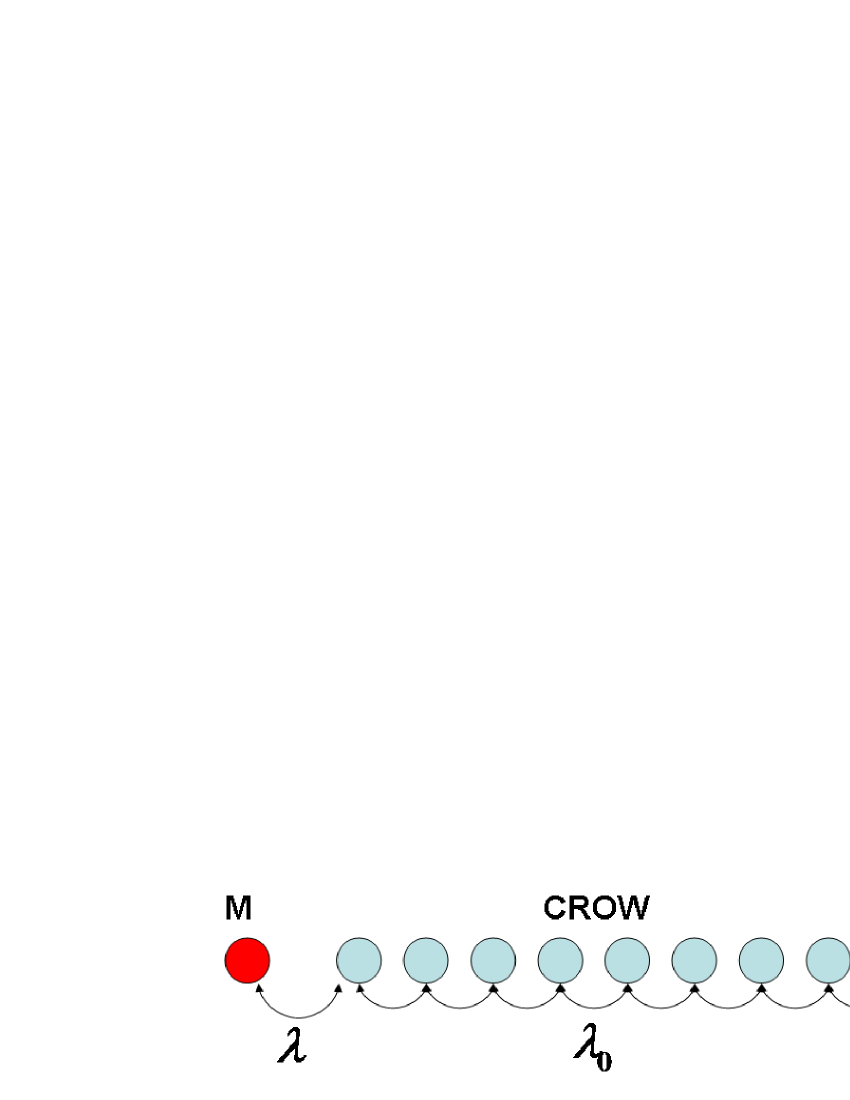
Figure 1: A schematic plot of a nanocavity (M) coupled to a CROW structure.

Consider the waveguide is semi-infinite long, then performing the following Fourier transformation $b_{k}=\sqrt{2/\pi}\sum_{n=1}^{\infty}\sin(nk)b_{n}$, where the operators $b_{k}$ and $b_{k}^{\dagger}$ correspond to the Bloch modes of the waveguide, the Hamiltonian of Eq. (19) becomes

$$H = \omega_{c}a^{\dagger}a+\sum_{k}\omega_{k}b_{k}^{\dagger}b_{k}+\sum_{k}g_{k}(ab_{k}^{\dagger}+b_{k}a^{\dagger}),$$ (20)

where

$$\omega_{k}=\omega_{0}-2\lambda_{0}\cos k~{},~{}~{}g_{k}=\sqrt{\frac{2}{\pi}}\lambda\sin k.$$ (21)

with $0\leq k\leq\pi$. As we see, Eq. (20) is reduced to the same form of Eq. (1) for the system considered in Secs. II-III.

IV.1 Initially system-reservoir correlated squeezed state

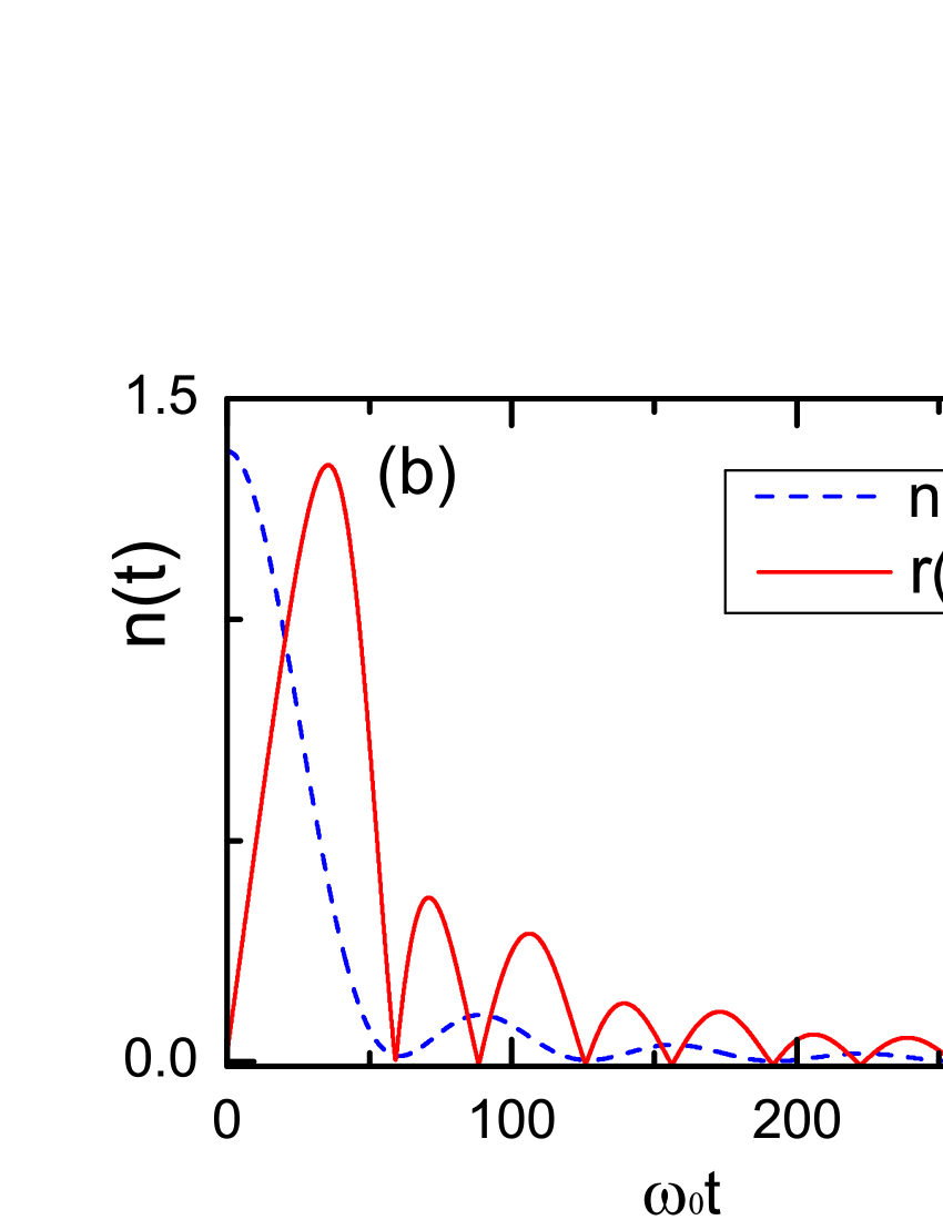
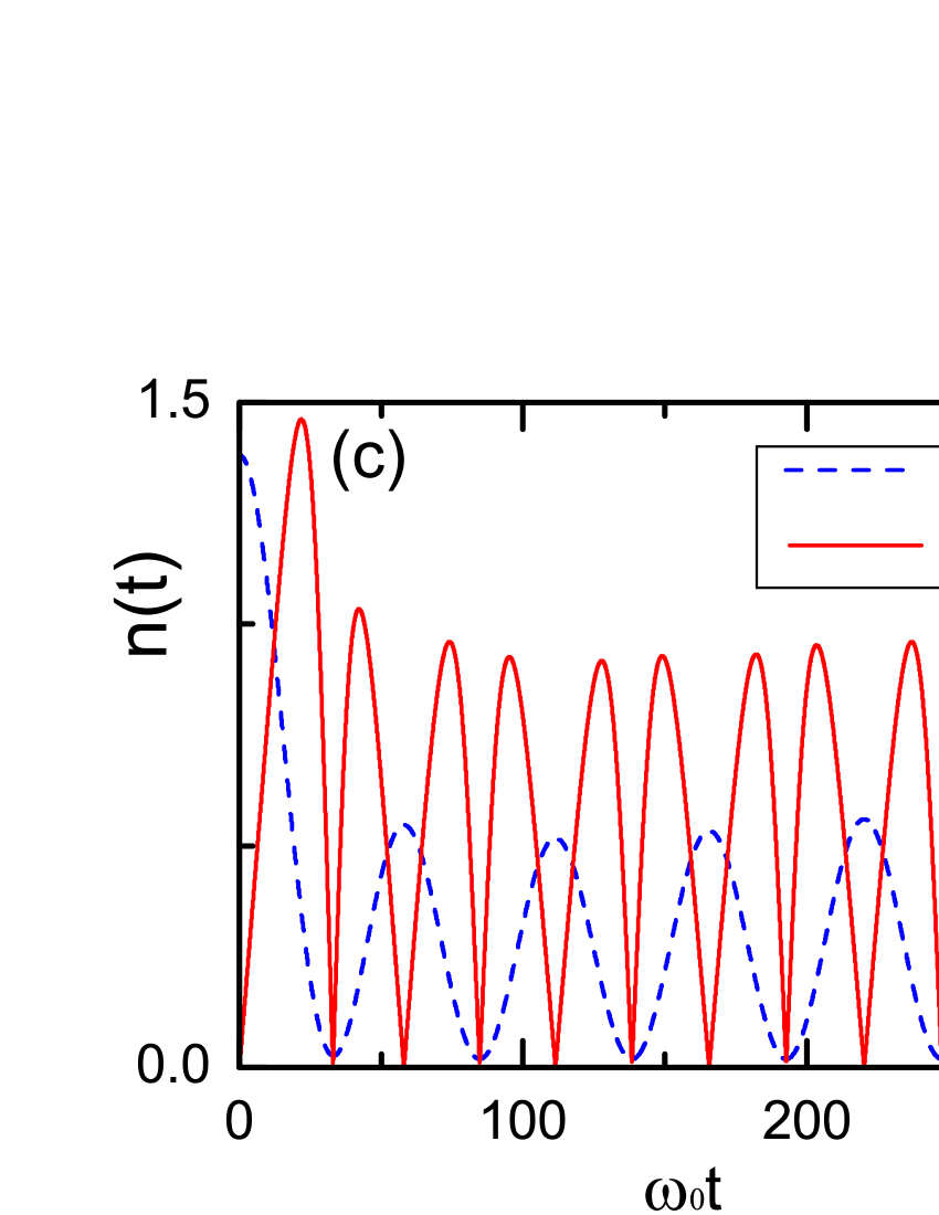
Figure 2: The time evolution of the cavity field intensity , i.e. the average photon number $n(t)=\langle a^{\dagger}(t)a(t)\rangle$ and the squeezing parameter $r(t)$ in the presence of the initial two-photon correlation between the system and the reservoir. The parameters taken in the plots are $\omega_{c}=\omega_{0}$, $\lambda_{0}=0.025\omega_{0}$, $r_{s}=1.0$, $\theta_{s}=0$, with $\eta=0.4$ in (a), $\eta=1.2$ in (b), and $\eta=2.0$ in (c).

For the above specific physical system, we shall first consider an initial system-reservoir correlated state with two-photon correlation $\langle a(0)b_{k}(0)\rangle\neq 0$. We assume that the cavity field is correlated initially with the first resonator mode of the CROW in terms of a two-mode entangled squeezed vacuum state TMSS1 as

$$|\psi_{ab_{1}}(0)\rangle=\exp(-r_{s}e^{-i\theta_{s}}ab_{1}+r_{s}e^{i\theta_{s}}a^{\dagger}b_{1}^{\dagger})|0_{a}0_{b_{1}}\rangle,$$ (22)

and the other resonators in the CROW are in vacuum, with $r_{s}$ and $\theta_{s}$ being the squeezing parameter and the reference phase, respectively. The strength of the nonclassical correlations (entanglement) contained in the above state increases with the increasing of the squeezing parameter $r_{s}$ TMSS2 . The reduced density matrices of the cavity field and the resonator mode from Eq. (22) is a mixed state which can be expressed as

$$\rho_{a/b_{1}}(0)=\sum_{n=0}^{\infty}\frac{\sinh^{2n}r_{s}}{(\sinh^{2}r_{s}+1)^{n+1}}|n_{a/b_{1}}\rangle\langle n_{a/b_{1}}|,$$ (23)

which is indeed of a single-mode thermal state with average thermal photon number $n_{a/b_{1}}(0)=\sinh^{2}r_{s}$. Based on the same Fourier transformation, it follows that the initial system-reservoir correlations are then given by

$$\langle a(0)b_{k}(0)\rangle=\sqrt{\frac{1}{2\pi}}\sinh 2r_{s}e^{i\theta_{s}}\sin k,$$ (24a)

$$\langle a(0)b_{k}^{\dagger}(0)\rangle=0,$$ (24b)

namely, the initial Gaussian state only has initial two-photon correlation between the system and the reservoir.

With the initial system-reservoir correlations in Eq. (24), we obtain from Eq. (10) that $\nu_{1}(t)=0=\upsilon_{0}(t)=\upsilon_{2}(t)$ and

$$\nu_{2}(t)=-i\frac{\sinh 2r_{s}e^{i\theta_{s}}}{\sqrt{2\pi}}\mathcal{F}(t),$$ (25a)

$$\upsilon_{1}(t)=\frac{2}{\pi}\sinh^{2}r_{s}|\mathcal{F}(t)|^{2},$$ (25b)

where

$$\mathcal{F}(t) =\int_{0}^{t}d\tau\sum_{k}g_{k}\sin(k)e^{-i\omega_{k}\tau}u(t-\tau)$$

$$=\frac{\eta}{\sqrt{2\pi}}\int_{0}^{t}d\tau\int_{0}^{\infty}d\omega\sin[k(\omega)]e^{-i\omega\tau}u(t-\tau).$$ (26)

The last line of the above equation has been applied to the waveguide band structure given in Eq. (21), so that $\eta=\frac{\lambda}{\lambda_{0}}$ and $\sin[k(\omega)]=\frac{1}{2\lambda_{0}}\sqrt{4\lambda_{0}^{2}-(\omega-\omega_{0})^{2}}$ with $\omega_{0}-2\lambda_{0}\leq\omega\leq\omega_{0}+2\lambda_{0}$.

After obtaining the time-dependent functions $\nu_{j}(t)$ and $\upsilon_{j}(t)$ given above, Eq. (9) becomes

$$\langle a(t)\rangle=0,$$ (27a)

$$n(t)=|u(t)|^{2}n_{a}(0)+\upsilon_{1}(t),$$ (27b)

$$s(t)=2u(t)\nu_{2}(t).$$ (27c)

This solution indicates that for the given initial thermal state $\rho_{a}(0)$ in Eq.(23), the cavity field at time $t$ is in a squeezed thermal state marian , which can be expressed as

$$\rho(t)=S_{a}[r(t)]\rho_{\rm th}(t)S_{a}^{\dagger}[r(t)],$$ (28)

where the single-mode squeezing operator

$$S_{a}[r(t)]=\exp[-\frac{r(t)}{2}e^{-i\theta(t)}a^{2}+\frac{r(t)}{2}e^{i\theta(t)}a^{{\dagger}2}],$$ (29)

with the squeezing parameters

$$r(t)=\frac{1}{4}\ln\frac{n(t)+|s(t)|+1/2}{n(t)-|s(t)|+1/2},$$ (30)

and $\theta(t)=\arg[s(t)]$. The thermal state

$$\rho_{\rm th}(t)=\sum_{k}\frac{[\bar{n}(t)]^{n}}{[\bar{n}(t)+1]^{k+1}}|n_{a}\rangle\langle n_{a}|,$$ (31)

where the average thermal photon number $\bar{n}(t)=\sqrt{(n(t)+1/2)^{2}-|s(t)|^{2}}-1/2$. By defining the quadrature operators $X=(a+a^{\dagger})/\sqrt{2}$ and $Y=(a-a^{\dagger})/\sqrt{2i}$, the covariance matrix are given by

$$\begin{pmatrix}\Delta X^{2}&\Delta\{XY\}\\ \Delta\{YX\}&\Delta Y^{2}\end{pmatrix}=\Big{[}\bar{n}(t)+\frac{1}{2}\Big{]}\Big{[}\frac{\cosh 2r(t)}{2}I~{}~{}$$

$$+\frac{\sinh 2r(t)}{2}\begin{pmatrix}\cos\theta(t)&\sin\theta(t)\\ \sin\theta(t)&-\cos\theta(t)\end{pmatrix}\Big{]}.$$ (32)

If $\bar{n}(t)=0$, the above covariance matrix is reduced to the standard form for a pure squeezed state Zhang90867 . Obviously, the squeezed thermal state squeezes the thermal-state fluctuation $\bar{n}(t)+1/2$. Thus, the squeezing in the squeezed thermal state can be described by the squeezing parameter $r(t)$. If there is no initial system-reservoir correlation, then we have $\nu_{2}(t)=0$ so that $s(t)=0$ which leads to the squeezing parameter $r(t)=0$.

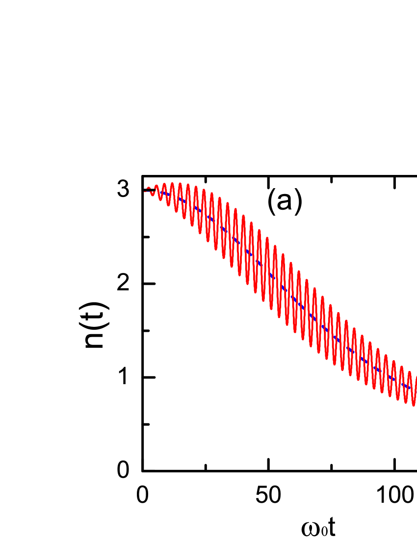
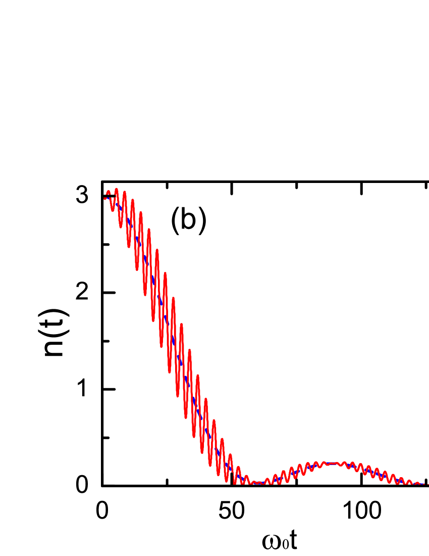
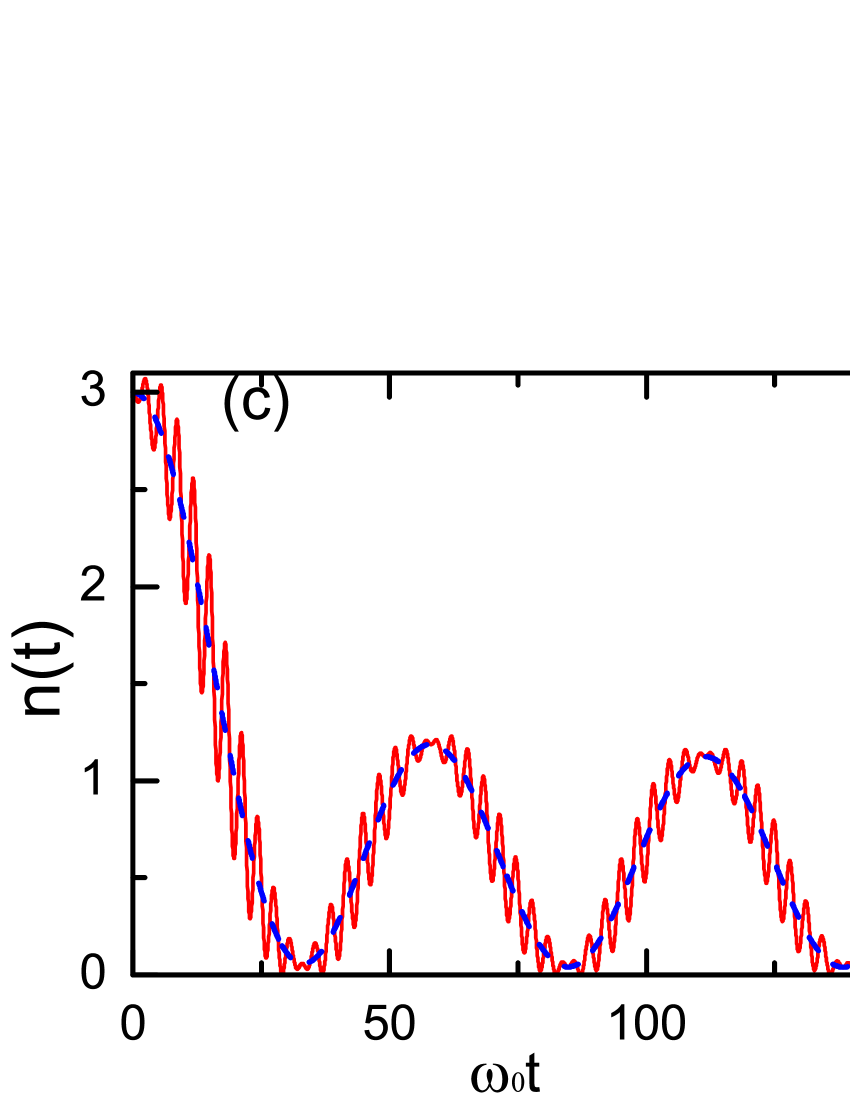
Figure 3: The time evolution of the cavity field intensity $n(t)$ with the initial correlation $\langle a(0)b_{1}^{\dagger}(0)\rangle$ (red solid line) and without such correlation (blue dashed line) for $\omega_{c}=\omega_{0}$, $\lambda_{0}=0.025\omega_{0}$, $\bar{n}_{a}=6$, $\bar{n}_{b_{1}}=0$, $\vartheta=\frac{\pi}{2}$, $\eta=0.4$ in (a), $\eta=1.2$ in (b), and $\eta=2.0$ in (c).

In Fig. 2, the time evolution of the cavity intensity $n(t)$ and the squeezing parameter $r(t)$ are plotted for the different coupling strengths $\eta=\lambda/\lambda_{0}$. As shown in Fig. 2 (a), for a weak coupling ($\eta=0.4$), the cavity intensity decays monotonically and eventually approaches to zero, as a result of the Markovian damping dynamics at zero temperature. Also, the small but non-zero squeezing parameter $r(t)$ indicates that the initial two-photon correlation $\langle a(0)b_{k}(0)\rangle$ between the system and reservoir induces a small squeezing effect to the cavity field in the beginning. However, the long-time behavior of the squeezing parameter shows that the effect of the initial system-reservoir correlation is washed out in the long-time limit, which is also consistent with the Markovian dynamics. In contrast, by increasing the coupling strength, as depicted in Fig. 2 (b), the cavity intensity decays rather fast in the beginning and then it revives and damps with oscillation in which some non-Markovian memory effect appears. Interestingly, the squeezing parameter $r(t)$ shows a similar behavior of the non-Markiovan effect, except for the beginning where the initial two-photon correlation $\langle a(0)b_{1}(0)\rangle$ generates a stronger squeezing effect to the cavity field, in comparison with the weak coupling case. When the coupling strength continues increasing to $\eta=2.0$ (the strong non-Markovian regime Wu1018407 ), the cavity intensity decays faster in the very beginning and then revives and keeps oscillating without damping from then on, see Fig. 2 (c). In this situation, we find that the initial-correlation-induced squeezing dynamics also oscillates over all the time. Therefore, we can conclude that the initial two-photon correlations $\langle a(0)b_{k}(0)\rangle$ can lead to a nontrivial squeezing dynamics of the cavity field, as a consequence of strong non-Markovian memory dynamics, but it is negligible in the steady-state limit in the Markovian regime.

IV.2 Initially system-reservoir correlated mixed thermal states

Next, we investigate the effect of the initially system-reservoir correlated state with the correlation $\langle a(0)b_{k}^{\dagger}(0)\rangle\neq 0$. To this end, we consider an initially mixed state

$$\rho_{ab_{1}}(0)=B(\vartheta)\rho_{a}\otimes\rho_{b_{1}}B^{\dagger}(\vartheta),$$ (33)

where the operator $B(\vartheta)=\exp[\frac{\vartheta}{2}(ab_{1}^{\dagger}-a^{\dagger}b_{1})]$ and the density operators $\rho_{a/b_{1}}$ represent the thermal states with average thermal photon numbers $\bar{n}_{a/b_{1}}$. This initially correlated state can be formed via the bilinear coupling between the cavity field $a$ and the resonator mode $b_{1}$ in the thermal states, and note that nonclassical entanglement are not present in this initially correlated state kim . A direct calculation shows that the initial system-reservoir correlations

$$\langle a(0)b_{k}(0)\rangle=0,$$ (34a)

$$\langle a(0)b_{k}^{\dagger}(0)\rangle=\frac{\sin\vartheta}{\sqrt{2\pi}}(\bar{n}_{a}-\bar{n}_{b_{1}})\sin k.$$ (34b)

For the initially correlated state of Eq.(33), it is easy to find that the reduced density matrices $\rho_{a}(0)$ and $\rho_{b_{1}}(0)$ of the cavity field and the resonator mode $b_{1}$ are also the thermal states with the average thermal photon numbers $n_{a}(0)=\frac{1}{2}[\bar{n}_{a}+\bar{n}_{b_{1}}+(\bar{n}_{a}-\bar{n}_{b_{1}})\cos\vartheta]$ and $n_{b_{1}}(0)=\frac{1}{2}[\bar{n}_{a}+\bar{n}_{b_{1}}-(\bar{n}_{a}-\bar{n}_{b_{1}})\cos\vartheta]$, respectively. From Eq.(10), we obtain

$$\nu_{1}(t) = -i\frac{(\bar{n}_{a}-\bar{n}_{b_{1}})\sin\vartheta}{\sqrt{2\pi}}\mathcal{F}(t),$$ (35)

$$\upsilon_{1}(t) = \frac{2n_{b_{1}}(0)}{\pi}|\mathcal{F}(t)|^{2},$$ (36)

and $\nu_{2}(t)=0$, and $\upsilon_{0}(t)=0$, $\upsilon_{2}(t)=0$. Thus, the corresponding physical observables of the cavity system for the above initially correlated state of Eq.(33) are given by

$$n(t)=|u(t)|^{2}n_{a}(0)+2Re[u^{*}(t)\nu_{1}(t)]+\upsilon_{1}(t),$$ (37)

and $\langle a(t)\rangle=0$, $s(t)=0$. It indicates that the cavity state remains in a thermal state over all the time with the cavity field intensity $\sim n(t)$.

In Fig. 3, the time evolution of the cavity field intensity $n(t)$ is plotted for different coupling strengths $\eta$ between the nanocavity and the waveguide. Fig. 3 (a) shows the the average photon number for a weak coupling $\eta=0.4$. It reveals that the intensity of the cavity field decays monotonically to a steady-state value, as a character of the Markovian dynamics. The initial system-reservoir correlation $\langle a(0)b_{k}^{\dagger}(0)\rangle$ leads to the intensity oscillating around the decay line of the case of the initially uncorrelated state. The amplitude of the local oscillations increases in the beginning and then decreases to a unnoticeable effect as time develops. In other words, the effect of the initial correlation $\langle a(0)b_{k}^{\dagger}(0)\rangle$ will be washed out in the steady limit. With the increasing of the coupling strength, the intensity no longer monotonically decays and some revival phenomena occur as a character of the non-Markovian memory dynamics Wu1018407 , as depicted in Fig. 3 (b). When the coupling is increased to $\eta=2.0$ as a strong coupling value, we see from Fig. 3 (c) that the intensity and the initial system-reservoir induced oscillation keep oscillating in the whole time regime. In other words, the effect resulted from the initial system-reservoir correlation in the non-Markovian regime will not be washed out by the interaction between the system and the reservoir.

V Summary

In summary, we investigate the dynamics of open quantum systems in the presence of initial system-reservoir correlations. We take the photonic cavity system coupled to a non-Markovian reservoir as a specific open quantum system. By solving the exact dynamics of the cavity system, the effects of the initial correlations are explicitly built into the solution of the cavity field intensity and the two-photon correlation function. We also derive the time-convolutionless exact master equation which incorporates with the initial system-reservoir correlations. The non-Markovian memory effects are fully embedded into the time-dependent coefficients in the master equation. The fluctuation coefficient $\gamma_{2}(t)$ is modified by the initial system-reservoir photonic scattering correlation but the frequency shift $\Delta(t)$ of the cavity and the dissipation coefficient $\gamma_{1}(t)$ remain unchanged. However, the initial two-photon correlation between the system and the reservoir induces two-photon decoherence terms in the master equation, which can lead to photon squeezing in the cavity. We also take a nanocavity coupled to a coupled resonator optical waveguide (serving as a structured reservoir) as an experimentally realizable system, from which we find that the effects of the initial correlations are fragile for a Markovian reservoir but play an important role in the non-Markovian regime. In fact, in the strong non-Markovian regime, the initial two-photon correlation between the cavity and the reservoir can induce oscillating squeezing dynamics in the cavity. But in Markovian regime, the effects of the initial system-reservoir correlations will be washed out in the steady-state limit.

References

- (1) H. J. Carmichael, An Open Systems Approach to Quantum Optics, Lecture Notes in Physics, Vol. m18 (Springer-Verlag, Berlin, 1993).
- (2) C. Cohen-Tannoudji, J. Dupont-Roc, and G. Grynberg, Atom and Photon Interactions: Basic Processes and Applications (Wiley, New York, 1998).
- (3) H. P. Breuer and F. Petruccione, The Theory of Open Quantum Systems (Oxford University Press, New York, 2007).
- (4) R. P. Feynman and F. L. Vernon, Ann. Phys. (NY) 24, 118 (1963).
- (5) A. O. Caldeira and A. J. Leggett, Physica A 121, 587 (1983).
- (6) F. Haake and R. Reibold, Phys. Rev. A 32, 2462 (1985).
- (7) B. L. Hu, J. P. Paz, and Y. H. Zhang, Phys. Rev. D 45, 2843 (1992).
- (8) J. J. Halliwell and T. Yu, Phys. Rev. D 53, 2012 (1996).
- (9) G. W. Ford and R. F. O’Connell, Phys. Rev. D 64, 105020 (2001).
- (10) L. Diósi, N. Gisin, and W. T. Strunz, Phys. Rev. A 58, 1699 (1998)
- (11) W. T. Strunz, L. Diosi, N. Gisin, and T. Yu, Phys. Rev. Lett. 83, 4909 (1999); W. T. Strunz and T. Yu, Phys. Rev. A 69, 052115 (2004).
- (12) T. Yu, Phys. Rev. A 69, 062107 (2004).
- (13) M. W. Y. Tu and W. M. Zhang, Phys. Rev. B 78, 235311 (2008).
- (14) M. W. Y. Tu, M. T. Lee, and W. M. Zhang, Quant. Info. Proc. 8, 631 (2009).
- (15) J. S. Jin, M. T. W. Tu, W. M. Zhang and Y. J. Yan, New J. Phys. 12, 083013 (2010)).
- (16) H. N. Xiong, W. M. Zhang, X. G. Wang, and M. H. Wu, Phys. Rev. A 82, 012105 (2010).
- (17) M. H. Wu, C. U. Lei, W. M. Zhang, and H. N. Xiong, Opt. Express 18, 18407 (2010).
- (18) C. U. Lei and W. M. Zhang, arXiv:1011.4570 (2010).
- (19) A. J. Leggett, S. Chakravarty, A. T. Dorsey, M. P. Fisher, A. Garg, and W. Zwerger, Rev. Mod. Phys. 59, 1 (1987).
- (20) A. Royer, Phys. Rev. Lett. 77, 3272 (1996).
- (21) V. Hakim and V. Ambegaokar, Phys. Rev. A 32, 423 (1985).
- (22) C. M. Smith and A. O. Caldeira, Phys. Rev. A 41, 3103 (1990).
- (23) R. Karrlein and H. Grabert, Phys. Rev. E 55, 153 (1997).
- (24) L. D. Romero and J. P. Paz, Phys. Rev. A 55, 4070 (1997).
- (25) E. Lutz, Phys. Rev. A 67, 022109 (2003).
- (26) E. Pollak, J. Shao, and D. H. Zhang, Phys. Rev. E 77, 021107 (2008).
- (27) E. M. Laine, J. Piilo, and H. P. Breuer, arXiv:1004.2184 (2010).
- (28) J. Dajka and J. Luczka, Phys. Rev. A 82, 012341 (2010).
- (29) K. Modi and E. C. G. Sudarshan, Phys. Rev. A 81, 052119 (2010).
- (30) Y. J. Zhang, X. B. Zou, Y. J. Xia, and G. C. Guo, Phys. Rev. A 82, 022108 (2010).
- (31) A. G. Dijkstra and Y. Tanimura, Phys. Rev. Lett. 104, 250401 (2010).
- (32) P. Lambropoulos, G. Nikolopoulos, T. R. Nielsen and S. Bay, Rep. Prog. Phys. 63, 455 (2000).
- (33) U. Fano, Phys. Rev. 124, 1866 (1961).
- (34) L. P. Kadanoff and G. Baym, Quantum Statistical Mechanics (Benjamin, New York, 1962).
- (35) J. H. An, and W. M. Zhang, Phys. Rev. A 76, 042127 (2007); J. H. An, M. Feng, and W. M. Zhang, Quantum Inf. Comput. 9, 0317 (2009).
- (36) S. Longhi, Phys. Rev. B 80, 165125 (2009).
- (37) D. F. Walls and G. J. Milburn, Quantum Optics (Springer-Verlag, Berlin, 1994).
- (38) G. X. Li, H. T. Tan, and S. Ke, Phys. Rev. A 74, 012304 (2006).
- (39) P. Marian, T. A. Marian, and H. Scutaru, Phys. Rev. Lett. 88, 153601 (2002).
- (40) W. M. Zhang, D. H. Feng, and R. Gilmore, Rev. Mod. Phys. 62, 867 (1990).
- (41) M. S. Kim, W. Son, V. Buzek, and P. L. Knight, Phys. Rev. A 65, 032323 (2002).