Thermoelectric effect of multiferroic oxide interfaces

Abstract

We investigate the thermoelectric properties of electrons at the interface of oxide heterostructure and in the presence of a multiferroic oxide with spiral spin order. We find there is no (spin) Hall current generated by the temperature gradient. A Seebeck effect is however present. Due to the magnetoelectric coupling, the charge and thermal conductivities are electrically controllable via the spin spiral helicity. Moreover, the thermopower exhibits a sign change when tuning electro-statically the carrier density.

The efficient manipulation of the spin-dependent transport properties of electronic systems is intensively studied due to its importance in spintronics applications. Thereby, a key role is played by the spin-orbit interaction (SOI); e.g. SOI is at the heart of the charge/spin Hall effect that have been successfully realized in different condensed matter Nagaosa . On the other hand, charge and spin currents can also be generated by a temperature gradient, a phenomena termed as the Seebeck and the spin-Seebeck effect, respectivelyBook-Marder ; SSE . Very recently, an intrinsic thermo-spin Hall effect has been predicted in a two-dimensional electron gas (2DEG) with finite Rashba SOI Ma-10 . A general theory of the thermal Hall effect in quantum magnets is developed by Katsura et.al. in Ref.[KNL, ]. The corresponding magnon Hall effect has been observed in Lu₂V₂O₇ with a pyrochlore structure Magon-HE . In this letter, we study the thermoelectronics of an interfacial quasi 2DEG formed at the junction of oxides LaTiO₃/SrTiO₃ or LaAlO₃/SrTiO₃ Oxides . As argued in JB ; HE-JB new functionalities are achieved when one of the oxide layer is multiferroic with a transverse spiral magnetic order, e.g. RMnO₃ (R=Tb, Dy, Gd) RMnO3 . We expect similar effects for compounds of the form LaAlO₃/SrTiO₃/RMnO₃ when SrTiO₃ is only few layers think. In that case the 2DEG at the interface of LaAlO₃/SrTiO₃ is expected to be influenced by the spiral order in RMnO₃. The essential point is that due to the topological structure of the local magnetic moments, a traversing carrier experiences an effective electrically controllable SOI. This SOI depends linearly on the carriers wave vector and on the helicity of the oxides magnetic order. Such an effective SOI is in a complete analogy to the semiconductor case where the RashbaRashba SOI and Dresselhaus Dresselhaus SOI have equal strengths, and results in an anisotropic charge and heat conductivities, which is tunable by a transversal electric field, and so is the thermopower.

The non-equlibrium current density in a system subject to potential $V$ and temperature $T$ gradients is phenomenologically given by Te_Jonson84 ,

$$\hat{J}^{(i)}_{\mu}=(1/e)\kappa_{\mu\nu}^{(ie)}\partial_{\nu}V+T\kappa_{\mu\nu}^{(iq)}\partial_{\nu}(1/T).$$ (1)

where $\mu$ and $\nu$ ($=x,y$) are spatial subscripts. $i$ stands for the subscripts $e$, $q$ and $s$ that denote respectively the charge, heat, and spin currents $\hat{\mbox{\boldmath$\mathrm{J}$}}^{(e)}$, $\hat{\mbox{\boldmath$\mathrm{J}$}}^{(q)}$, and $\hat{\mbox{\boldmath$\mathrm{J}$}}^{(s)}$. Those are defined as

$$\hat{\mbox{\boldmath$\mathrm{v}$}}=\delta H_{0}/\delta\mbox{\boldmath$\mathrm{P}$},\;\hat{\mbox{\boldmath$\mathrm{J}$}}^{(e)}=e\hat{\mbox{\boldmath$\mathrm{v}$}}$$ (2)

$$\hat{\mbox{\boldmath$\mathrm{J}$}}^{(q)}=\frac{1}{2}\{H_{0},\hat{\mbox{\boldmath$\mathrm{v}$}}\}-E_{f}\hat{\mbox{\boldmath$\mathrm{v}$}},$$ (3)

$$\hat{\mbox{\boldmath$\mathrm{J}$}}^{(s)}=\frac{\hbar}{4}\{\mbox{\boldmath$\mathrm{\sigma}$},\hat{\mbox{\boldmath$\mathrm{v}$}}\}.$$ (4)

Here $H_{0}$ is the unperturbed Hamiltonian, $\mathrm{P}$ is the momentum operator, $\mathrm{\sigma}$ is the vector of Pauli matrices, and $E_{f}$ is the chemical potential of the system. The Seebeck coefficient $S_{\mu\nu}=-\partial_{\mu}V/\partial_{\nu}T$ is given by the zero charge-current condition satisfying

$$S_{\mu\nu}=(-e/T)\kappa_{\mu\gamma}^{(eq)}/\kappa_{\gamma\nu}^{(ee)}.$$ (5)

Considering a spatial homogeneous electric field and a temperature gradient, the vector potentials read $\mbox{\boldmath$\mathrm{A}$}^{(e)}=\mbox{\boldmath$\mathrm{E}$}e^{-i\omega t}/i\omega$ and $\mbox{\boldmath$\mathrm{A}$}^{(q)}=-\nabla T/Te^{-i\omega t}/i\omega$, respectively. Following Luttinger Luttinger , all the response functions can be obtained from the Kubo formula Te_Jonson84 ; Book_Coleman

$$\kappa_{\mu\nu}^{(ij)}(\omega) = \frac{i}{\hbar\omega}\int_{0}^{\hbar\beta}d\tau e^{i\omega\tau}\langle T\hat{J}_{\mu}^{(i)}(\tau)\hat{J}_{\nu}^{(j)}(0)\rangle$$ (6)

$$= \frac{1}{i\omega\beta}\sum_{mn}\langle\psi_{m}|\hat{J}_{\mu}^{(i)}|\psi_{n}\rangle\langle\psi_{n}|\hat{J}_{\nu}^{(j)}|\psi_{m}\rangle$$

$$\times \sum_{p}G_{n}(ip+i\omega)G_{m}(ip),$$

where $G$ is the Matsubara Green function and only the loop diagram contributing to the current fluctuations is taken into account Book_Coleman . Performing the Matsubara sum over $ip$, we have

$$\kappa_{\mu\nu}^{(ij)}(\omega)=\frac{1}{i\omega}\sum_{mn}\frac{[f(E_{m})-f(E_{n})](\hat{J}_{\mu}^{(i)})_{mn}(\hat{J}_{\nu}^{(j)})_{nm}}{E_{m}-E_{n}+\omega+i\Gamma}$$ (7)

with $\Gamma$ being the relaxation rate. By using the following relation between the corresponding matrix elements,

$$\langle\psi_{n}|\mbox{\boldmath$\mathrm{v}$}|\psi_{m}\rangle=\frac{i}{\hbar}(E_{n}-E_{m})\langle\psi_{n}|\mbox{\boldmath$\mathrm{r}$}|\psi_{m}\rangle$$ (8)

the conductivity is obtained in the static limit Nagaosa ; Sinova-04 ,

$$\sigma_{\mu\nu}^{(ij)}=\text{Im}\sum_{m\neq n}\frac{f(E_{m})-f(E_{n})}{(E_{m}-E_{n})/\hbar}\frac{(\hat{J}_{\mu}^{(i)})_{mn}(\hat{J}_{\nu}^{(j)})_{nm}}{E_{m}-E_{n}+i\Gamma}$$ (9)

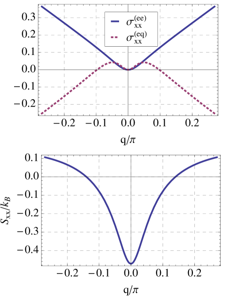
Figure 1: (Top) Charge $\sigma_{xx}^{ee}$[$e^{2}/2\pi h$] and thermal $\sigma_{xx}^{eq}$ [$(e\hbar/2ma^{2})(1/2\pi)^{4})$] conductivity. (Bottom) the thermopower as a function of the spiral spin wave vector $q$, where $a$ is the lattice constant and $k_{B}$ is Boltzmann constant. Parameters are chosen such that $U=0.1$, $E_{f}=0.2$, $\Gamma=0.05$ and $k_{B}T=0.1$. All measured in the unit of energy $\epsilon_{0}=\hbar^{2}/2ma^{2}$.

Our specific system is the two-dimensional electron gas (2DEG) influenced by a spiral multiferroic oxide, as discussed above. The coupling between the local spiral magnetic moments ($\mbox{\boldmath$\mathrm{m}$}_{r}$ $=[\sin\theta_{r},0,\cos\theta_{r}]$ where $\theta_{r}=\mbox{\boldmath$\mathrm{q}$}_{m}\cdot\mbox{\boldmath$\mathrm{r}$}$ with $\mbox{\boldmath$\mathrm{q}$}_{m}=[q,0,0]$) to the conduction electrons is governed by the $sd$ Hamiltonian JB ,

$$H=h_{k}+h_{sd}=\frac{1}{2m}\mbox{\boldmath$\mathrm{P}$}^{2}+U\mbox{\boldmath$\mathrm{n}$}_{r}\cdot\mbox{\boldmath$\mathrm{\sigma}$}.$$ (10)

After applying an unitary local gauge transformation in the spin space $U_{g}=e^{-i{\theta_{r}}\sigma_{y}/2}$, we get

$$H=\frac{1}{2m}(\mbox{\boldmath$\mathrm{P}$}+\mbox{\boldmath$\mathrm{A}$}_{g})^{2}+U\tilde{\sigma}_{z}$$ (11)

where $\mbox{\boldmath$\mathrm{A}$}_{g}=-i\hbar U_{g}^{\dagger}\nabla_{\mbox{\boldmath$\mathrm{r}$}}U_{g}=(-\hbar q\tilde{\sigma}_{y}/2)\hat{e}_{x}$ is the topological vector potential (hereafter, transformed quantities have a tilde). Explicitly diagonalizing the Hamiltonian (11) we obtain the eigenenergies

$$E_{\pm}(\mbox{\boldmath$\mathrm{k}$})=\frac{\hbar^{2}\mbox{\boldmath$\mathrm{k}$}^{2}}{2m}\pm\sqrt{U^{2}+(\frac{\hbar^{2}qk_{x}}{2m})^{2}}$$ (12)

with the eigenstates

$$|\psi_{+}\rangle=e^{-i\mbox{\boldmath$\mathrm{k}$}\cdot\mbox{\boldmath$\mathrm{r}$}}\left(\begin{array}[]{cc}\cos\frac{\phi}{2}\\ i\sin\frac{\phi}{2}\end{array}\right),\;|\psi_{-}\rangle=e^{-i\mbox{\boldmath$\mathrm{k}$}\cdot\mbox{\boldmath$\mathrm{r}$}}\left(\begin{array}[]{cc}i\sin\frac{\phi}{2}\\ \cos\frac{\phi}{2}\end{array}\right)$$ (17)

where

$$\tan\phi=\frac{\hbar^{2}qk_{x}}{2mU},\;\;\cos\phi=\frac{U}{\sqrt{U^{2}+(\frac{\hbar^{2}qk_{x}}{2m})^{2}}}.$$ (18)

The velocity operators then read,

$$\hat{v}_{x}=-i\frac{\hbar}{m}\overleftrightarrow{\nabla}_{x}-\frac{\hbar q\tilde{\sigma}_{y}}{2m},\;\hat{v}_{y}=-i\frac{\hbar}{m}\overleftrightarrow{\nabla}_{y}$$ (19)

where $\overleftrightarrow{\nabla}=(\overrightarrow{\nabla}-\overleftarrow{\nabla})/2$ is the symmetrized derivative. The topological vector potential $\mbox{\boldmath$\mathrm{A}$}_{g}$ introduces an extra dynamical diamagnetic response (the last term of $\hat{v}_{x}$) to all currents. However, different from the case of 2DEG embedded in a magnetic filed Te_Jonson84 , the corresponding dia-thermal current has zero equilibrium expectation value since $\langle\tilde{\sigma}_{y}\rangle=0$, whereas there is a persistent dia-spin current $\langle\hat{J}^{(s)}_{x}\rangle$ along the the spin wave vector of the spiral JB . Both the charge ($\langle\hat{J}^{(e)}_{\mu}\rangle$) and the heat ($\langle\hat{J}^{(q)}_{\mu}\rangle$) currents are generated along the direction of the external electric field and temperature gradient. We have just the Seebeck effect in absence of the spin-Seebeck effect.

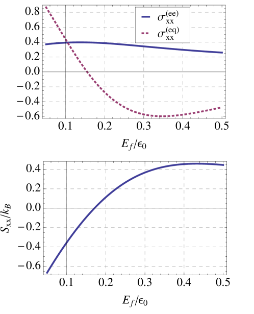
Figure 2: (Top) Charge $\sigma_{xx}^{ee}$[$e^{2}/2\pi h$] and thermal $\sigma_{xx}^{eq}$[$(e\hbar/2ma^{2})(1/2\pi)^{4}]$ conductivity and (bottom) the Seebeck coefficient $S_{xx}$ vs. chemical potential $E_{f}$ with the spiral helicity $q=2\pi/7$. Other parameters are same as in Fig.1.

Now let’s consider the transport properties. It is straightforward to work out that the only nonzero matrix elements are

$$\langle\psi_{+}|\hat{J}_{x}^{(e)}|\psi_{-}\rangle=ie\frac{\hbar q}{2m}\cos\phi,$$ (20)

$$\langle\psi_{+}|\hat{J}_{x}^{(q)}|\psi_{-}\rangle=i\frac{\hbar q}{2m}(\frac{\hbar^{2}\mbox{\boldmath$\mathrm{k}$}^{2}}{2m}-E_{f})\cos\phi,$$ (21)

$$\langle\psi_{+}|\hat{J}_{\mu}^{(s)}|\psi_{-}\rangle=i\frac{\hbar^{2}k_{\mu}}{2m}\cos\phi.$$ (22)

which results in

$$\sigma_{\mu\nu}^{(sj)}\equiv 0\;\text{and }\sigma_{y\mu}^{(eq/qe)}\equiv 0.$$ (23)

No Hall current is induced by the external electric field nor by the temperature gradient because of the disappearance of the Berry phase Nagaosa ; Sinova-04 ; Shen-04 due to the resonant form of the eigenstates as a results of the coplanar spiral magnetic moments JB . The charge and the heat conductivity is anisotropic, only the diagonal component of the conductivities is nonzero. That is is sharp contrast to the semiconductor 2DEG with equal Rashba and Dresselhaus SOI leading to an isotropic conductivity MH-03 ; MBM-06 . The non-vanishing components of the conductivity tensors are presented in Fig.1. It should be noted that, due to the presence of the magneto-electric coupling, all transport properties are tunable by a small transverse electric field ($\sim$ 1kV/cm) which tunes the spin helicity $q$ E-Control-1 . For a large electric field, the FE polarization is stabilized, but the concentration of carriers at the interface is modulated E-Control-2 . We thus have an electrically controlled chemical potential, which results in a sign change of the thermal conductivity and of the Seebeck coefficient (see Fig.2).

When the oxide magnetic moments possess a small deviation from the spiral plane, the scalar spin chirality defined as the mixed product of three spins on a certain plaquette, $\chi_{ijk}=\mbox{\boldmath$\mathrm{S}$}_{i}\cdot(\mbox{\boldmath$\mathrm{S}$}_{j}\times\mbox{\boldmath$\mathrm{S}$}_{k})$ becomes nonzero. $\chi_{ijk}$ introduces a fictitious magnetic flux to the conduction electrons and provides a nontrivial Berry curvature of the wave function, leading to nonzero charge/spin JB ; Kagome and thermal KNL Hall conductivity.

References

• (1) N. Nagaosa, J. Phys. Soc. Jap. 75, 042001 (2006); J. Phys. Soc. Jap. 77, 031010 (2008).
• (2) M. P. Marder, Condensed Matter Physics, 451-462(John Wiley & Sons. Inc. 2000).
• (3) K. Uchida, S. Takahashi, K. Harii, J. Ieda, W. Koshibae, K. Ando, S. Maekawa, E. Saitoh, Nature 455, 778 (2008). K. Uchida , T. Ota, K. Harii, S. Takahashi, S. Maekawa, Y. Fujikawa, E. Saitoh, Solid State Commun. 150, 524 (2010); K. Uchida , T. Ota, K. Harii, K. Ando, H. Nakayama, and E. Saitoh, J. Appl. Phys. 107, 09A951 (2010).
• (4) Z.-S. Ma, Solid State Comm. 150, 510 (2010).
• (5) H. Katsura, N. Nagaosa, and P. A. Lee, Phys. Rev. Lett. 104, 066403 (2010).
• (6) Y. Onose, T. Ideue, H. Katsura, Y. Shiomi, N. Nagaosa, and Y. Tokura, Science 329, 297 (2010).
• (7) A. Ohtomo, D. A. Muller, J. L. Grazul, and H. Y. Hwang, Nature 419, 378 (2002); C. H. Ahn, J.-M. Triscone and J. Mannhart, Nature 424, 1015 (2003); J. Mannhart, D. H. A. Blank, H. Y. Hwang, A. J. Millis, and J.-M. Triscone, MRS Bulletin. 33 1027 (2008);
• (8) C.L. Jia and J. Berakdar, Phys. Rev. B 80, 014432 (2009); Appl. Phys. Lett. 95, 012105 (2009).
• (9) C.L. Jia and J. Berakdar, unpublished (2010).
• (10) Y. Tokura and S. Seki, Adv. Mater. 21, 1 (2009).
• (11) Y. A. Bychkov, E. I. Rashba, J. Phys. C 17, 6039 (1984).
• (12) G. Dresselhaus, Phys. Rev. 100, 580 (1955).
• (13) M. Jonson and S. M. Girvin, Phys. Rev. B 29, 1939 (1984).
• (14) J. M. Luttinger, Phys. Rev. B 135, 1505 (1964).
• (15) P. Coleman, Introduction to Many Body Physics, (http://www.physics.rutgers.edu/~coleman/, 2010).
• (16) N. S. Sinistyn, E. M. Hankiewicz, W. Teizer, and J. Sinova, Phys. Rev. B 70, 081312 (2004).
• (17) S.-Q. Shen, Phys. Rev. B 70, 081311 (2004).
• (18) E. G. Mishchenko and B. I. Halperin, Phys. Rev. B 68, 045317 (2003).
• (19) JesΓΊs A. Maytorena, Catalina LΓ³pez-Bastidas, and F. Mireless, Phys. Rev. B 74, 235313 (2006).
• (20) Y. Yamasaki, H. Sagayama, T. Goto, M. Matsuura, K. Hirota, T. Arima, and Y. Tokura, Phys. Rev. Lett. 98 147204 (2007); S. Seki, Y. Yamasaki, M. Soda, M. Matsuura, K. Hirota, and Y. Tokura, Phys. Rev. Lett. 100, 127201 (2008).
• (21) A.D. Caviglia, S. Gariglio, N. Reyren, D. Jaccard, T. Schneider, M. Gabay, S. Thiel, G. Hammerl, J. Mannhart, and J.-M. Triscone, Nature (London) 456, 624 (2008).
• (22) K. Ohgushi, S. Murakami, and N. Nagaosa, Phys. Rev. B 62, R6065 (2000); M. Taillefumier, B. Canals, C. Lacroix, V. K. Dugaev, and P. Bruno, Phys. Rev. B 74, 085105 (2006).