A Simple and Practical Algorithm
for Differentially Private Data Release

Abstract

We present a new algorithm for differentially private data release, based on a simple combination of the Exponential Mechanism with the Multiplicative Weights update rule. Our MWEM algorithm achieves what are the best known and nearly optimal theoretical guarantees, while at the same time being simple to implement and experimentally more accurate on actual data sets than existing techniques.

1 Introduction

Sensitive statistical data on individuals are ubiquitous, and publishable analysis of such private data is an important objective. When releasing statistics or synthetic data based on sensitive data sets, one must balance the inherent tradeoff between the usefulness of the released information and the privacy of the affected individuals. Against this backdrop, differential privacy [4, 11, 5] has emerged as a compelling privacy definition that allows one to understand this tradeoff via formal, provable guarantees. In recent years, the theoretical literature on differential privacy has provided a large repertoire of techniques for achieving the definition in a variety of settings (see, e.g., [8, 9]). However, data analysts have found that several algorithms for achieving differential privacy add unacceptable levels of noise.

In this work we develop a broadly applicable, simple, and easy-to-implement algorithm, capable of substantially improving performance on many realistic datasets. The algorithm is a combination of the Multiplicative Weights approach of [16, 15], maintaining and correcting an approximating dataset through queries on which the approximate and true datasets differ, and the Exponential Mechanism [22], which selects the queries most informative to the Multiplicative Weights algorithm (specifically, those most incorrect vis-a-vis the current approximation). While in the worst case one must separately measure all required queries, for less adversarial data and query sets our approximation can provide very accurate answers to all queries, having privately measured only a relatively small subset of them.

1.1 Our Results

We present MWEM, a new differentially private algorithm producing synthetic datasets (formally: a fractional weighting of the domain) respecting any set of linear queries (those that apply a function to each record and sum the results). Our algorithm matches the best known (and nearly optimal) theoretical accuracy guarantees for releasing differentially private answers to a set of counting queries (those mapping records to $\{0,1\})$.

We present experimental results for producing differentially private synthetic data for a variety of problems studied in prior work, based on a variety of real-world data sets. In each case, we empirically evaluate the accuracy of the differentially private data produced by MWEM using the same query class and accuracy metric proposed by the corresponding prior work.

1. We consider range queries as studied by [19, 20], and find up to three orders of magnitude improvements in accuracy for fixed privacy parameters across several datasets.

2. We investigate contingency table release across a collection of statistical benchmarks as in [13] and find we are able to improve on prior work for each.

3. We consider datacube release as studied by [3] and find that our general-purpose algorithm improves on specialized algorithms designed to optimize various criteria.

Releasing synthetic data guarantees important properties, including consistency of statistics and compatibility with downstream analyses expecting actual datasets as input.

Finally, we describe a scalable implementation of MWEM capable of processing and releasing datasets of substantial complexity. Producing synthetic data for the classes of queries we consider is known to be computationally hard in the worst-case [10, 24]. Indeed, almost all prior work performs computation proportional to the size of the data domain, which limits them to datasets with relatively few attributes. In contrast, we are able to process datasets with thousands of attributes, corresponding to domains of size $2^{1000}$. Our implementation integrates a scalable parallel implementation of Multiplicative Weights, and a representation of the approximating dataset in a factored form that only exhibits complexity when the model requires it.

2 Our Approach

MWEM maintains an approximating dataset as a (scaled) distribution over the domain $D$ of data records. We repeatedly improve the accuracy of this approximation with respect to the private dataset and the desired query set by selecting and posing a query poorly served by our approximation and improving the approximation to better reflect the answer to this query. We select and pose queries using the Exponential [22] and Laplace Mechanisms [5], whose definitions and privacy properties we review in Subsection 2.1. We improve our approximation using the Multiplicative Weights update rule [16], reviewed in Subsection 2.2. We describe their integration in Subsection 2.3, giving a full description of our algorithm and its formal properties.

2.1 Differential Privacy and Mechanisms

Differential privacy is a constraint on a randomized computation that the computation should not reveal specifics of individual records present in the input. It places this constraint by requiring the mechanism to behave almost identically on any two datasets that are sufficiently close.

Imagine a dataset $A$ whose records are drawn from some abstract domain $D$, and which is described as a function from $D$ to the natural numbers $\mathbb{N}$, with $A(x)$ indicating the frequency (number of occurrences) of $x$ in the dataset. We use $\|A-B\|$ to indicate the sum of the absolute values of difference in frequencies (how many records would have to be added and removed to change $A$ into another dataset $B$).

Definition 2.1 (Differential Privacy)

A mechanism $M$ mapping datasets to distributions over an output space $R$ provides $(\varepsilon,\delta)$-differential privacy if for every $S\subseteq R$ and for all data sets $A,B$ where $\|A-B\|\leq 1$,

$$\operatorname*{\mathbb{P}r}[M(A)\in S]\leq e^{\varepsilon}\operatorname*{\mathbb{P}r}[M(B)\in S]+\delta\;.$$

If $\delta=0$ we say that $M$ provides $\varepsilon$-differential privacy.

The Exponential Mechanism [22] is an $\varepsilon$-differentially private mechanism that can be used to select among the best of a discrete set of alternatives, where “best” is defined by a function relating each alternative to the underlying secret data. Formally, for a set of alternative results $R$, we require a quality scoring function $s:dataset\times R\rightarrow\mathbb{R}$, where $s(B,r)$ is interpreted as the quality of the result $r$ for the dataset $B$. To guarantee $\varepsilon$-differential privacy, the quality function is required to satisfy a stability property: that for each result r the difference $|s(A,r)-s(B,r)|$ is at most $\|A-B\|$. With this quality function in hand, the Exponential Mechanism $E$ simply selects a result $r$ from the distribution satisfying

$$\operatorname*{\mathbb{P}r}[E(B)=r]\propto\exp(\varepsilon\times s(B,r)/2).$$

Intuitively, the mechanism selects result $r$ biased exponentially by its quality score. The Exponential Mechanism takes time linear in the number of possible results, as it needs to evaluate $s(B,r)$ once for each $r$.

The Laplace Mechanism is an $\varepsilon$-differentially private mechanism which reports approximate sums of bounded functions across a dataset. If $f$ is a function from records to the interval $[-1,+1]$, the Laplace Mechanism $L$ obeys

$$\operatorname*{\mathbb{P}r}[L(B)=r]\propto\exp\big{(}-\varepsilon\times|r-\sum_{x\in D}f(x)\times B(x)|\big{)}\;.$$

Although the Laplace Mechanism is an instance of the Exponential Mechanism, it can be implemented much more efficiently, by adding Laplace noise with parameter $1/\varepsilon$ to the sum $\sum_{x\in D}f(x)\times B(x)$. As the Laplace distribution is exponentially concentrated, the Laplace Mechanism provides an excellent approximation to the true sum.

2.2 Multiplicative Weights Update Rule

The Multiplicative Weights approach has seen application in many areas of computer science. Here we will use it as proposed in Hardt and Rothblum [16], to repeatedly improve an approximate distribution to better reflect some true distribution. The intuition behind Multiplicative Weights is that should we find a query whose answer on the true data is much larger than its answer or the approximate data, we should scale up the approximating Weights on records contributing positively and scale down the Weights on records contributing negatively. If the true answer is much less than the approximate answer, we should do the opposite.

More formally, let $q$ be a function mapping records to the interval $[-1,+1]$, and extended to a function of datasets by accumulating the sum of $q$ applied to the individual records. If $A$ and $B$ are distributions over the domain $D$ of records, where $A$ is a synthetic distribution intended to approximate a true distribution $B$ with respect to query $q$, then the Multiplicative Weights update rule recommends updating the weight $A$ places on each record $x$ by:

$$A_{new}(x)\propto A(x)\times\exp(q(x)\times(q(B)-q(A))/2)\;.$$

The proportionality sign indicates that the approximation should be renormalized after scaling. Hardt and Rothblum show that each time this rule is applied, the relative entropy between $A$ and $B$ decreases by an additive $(q(A)-q(B))^{2}$. As long as we can continue to find queries on which the two disagree, we can continue to improve the approximation.

Although our algorithm will manipulate datasets, we can divide their frequencies by the numbers of records $n$ whenever we need to apply Multiplicative Weights updates, and renormalize to a fixed number of records (rather than to one, as we would for a distribution).

2.3 Putting Things Together

Our combined approach is simple: we repeatedly use the Exponential Mechanism to find queries $q$ that are poorly served by our current approximation of the underlying private data, we measure these queries using the Laplace Mechanism, and we then use this measurement to improve our distribution using the Multiplicative Weights update rule.

We assume there exists a set $Q$ of queries $q$, each functions from the record domain $D$ to the interval $[-1,+1]$ and extended to datasets $A$ by $q(A)=\sum_{x\in D}q(x)\times A(x)$. The MWEM algorithm appears in Figure 1.

 . Inputs: Data set $B$ over a universe $D,$

Inputs: Number of iterations $T\in\mathbb{N},$
Inputs: Privacy parameter $\varepsilon>0.$

Let $n$ denote $\|B\|$, the number of records in $B$.

Let $A_{0}$ denote $n$ times the uniform distribution over $D$.

For iteration $i=1,...,T$:

1. Exponential Mechanism: Sample a query $q_{i}\in Q$ using the Exponential Mechanism parametrized with epsilon value $\varepsilon/2T$ and the score function

   $$s_{i}(B,q)=|q(A_{i-1})-q(B)|\;.$$

2. Laplace Mechanism: Let measurement $m_{i}=q_{i}(B)+\mathit{Lap}(2T/\varepsilon).$

3. Multiplicative Weights: Let $A_{i}$ be $n$ times the distribution whose entries satisfy

   $$A_{i}(x)\propto A_{i-1}(x)\times\exp(q_{i}(x)\times(m_{i}-q_{i}(A_{i-1}))/2n)\;.$$

Output: $A=\mathop{\textrm{avg}}_{i<T}A_{i}.$

.  .

Figure 1: The MWEM algorithm.

To clarify how MWEM works, and to highlight its simplicity, we present a full implementation in the Appendix, in Figure 8.

2.3.1 Formal Guarantees

As indicated in the introduction, the formal guarantees of MWEM represent the best known theoretical results on differentially private synthetic data release.

We first describe the privacy properties of our algorithm.

Theorem 2.1

MWEM satisfies $\varepsilon$-differential privacy.

Proof 2.2.

The composition rules for differential privacy state that $\varepsilon$ values accumulate additively. We make $T$ calls to the Exponential Mechanism with parameter $(\varepsilon/2T)$ and $T$ calls to the Laplace Mechanism with parameter $(\varepsilon/2T)$, resulting in $\varepsilon$-differential privacy.

We now bound the worst-case performance of the algorithm, in terms of the maximum error between $A$ and $B$ across all $q\in Q$. The natural range for $q(A)$ is $[-n,+n]$, and we see that by increasing $T$ beyond $4\log|D|$ we can bring the error asymptotically smaller than $n$.

Theorem 2.3.

For any dataset $B$, set of linear queries $Q$, $T\in\mathbb{N}$, and $\varepsilon>0$, with probability at least $1-2T/|Q|$, MWEM produces $A$ such that

$$\max_{q\in Q}|q(A)-q(B)|\leq 2n\sqrt{\frac{\log|D|}{T}}+\frac{10T\log|Q|}{\varepsilon}\;.$$

Proof 2.4.

The proof of this theorem is an integration of pre-existing analyses of both the Exponential Mechanism and the Multiplicative Weights update rule. We include it for completeness in the Appendix.

By optimizing the choice of $T$ to minimize the above bound we have the following corollary, stated asymptotically only because the constants are messy rather than large.

Corollary 2.5.

For any $B$, $Q$, and $\varepsilon>0$, there exists a $T$ such that with probability at least $1-1/poly(|Q|)$, the $A$ returned by MWEM obeys

$$\max_{q\in Q}|q(A)-q(B)|\textrm{ is }O\left(n^{2/3}\left(\frac{\log|D|\log|Q|}{\varepsilon}\right)^{1/3}\right)\,.$$

If we permit $(\varepsilon,\delta)$-differential privacy with $\delta>0$, we can use k-fold adaptive composition [12] to conclude that MWEM also provides $(\varepsilon\sqrt{2\log(1/\delta)/T}+\varepsilon(e^{\varepsilon/T}-1),\delta)$-differential privacy, resulting in a different optimal $T$.

Corollary 2.6.

For any $B$, $Q$, and $\varepsilon^{\prime}>0,\delta>0$, there exist $\varepsilon>0$ and $T$ so that MWEM provides $(\varepsilon^{\prime},\delta)$-differential privacy and with probability at least $1-1/poly(|Q|)$ produces $A$ such that

$$\max_{q\in Q}|q(A)-q(B)|\textrm{ is }O\left(n^{1/2}\left(\frac{\log^{1/2}|D|\log|Q|\log(1/\delta)}{\varepsilon^{\prime}}\right)^{1/2}\right)\,.$$

Corollary 2.6 is tight in its dependence on $n$ and $|Q|.$ Indeed, there is a lower bound of $\Omega(\sqrt{n\log|Q|})$ on the error of any algorithm avoiding what is called “blatant non-privacy” [4, 11, 7]. As $(\varepsilon,\delta)$-differential privacy avoids blatant non-privacy for sufficiently small but constant $\varepsilon,\delta,$ the bound applies. We remark that the lower bound coincides with what is known as the statistical sampling error that arises already in the absence of any privacy concerns.

Note that these bounds are worst-case bounds, over adversarially chosen data and query sets. We will see in Section 3 that MWEM works very well in more realistic settings.

2.3.2 Running time

The running time of our basic algorithm as described in Figure 1 is $O(n|Q|+T|D||Q|)).$ The algorithm is embarrassingly parallel: query evaluation can be conducted independently, implemented using modern database technology; the only required serialization is that the $T$ steps must proceed in sequence, but within each step essentially all work is parallelizable.

Results of Dwork et al. [6] show that for worst case data, producing differentially private synthetic data for a set of counting queries requires time $|D|^{0.99}$ under reasonable cryptographic hardness assumptions. Moreover, Ullman and Vadhan [24] showed that similar lower bounds also hold for more basic query classes such as we consider in Section 3.2. Despite these hardness results, we provide an alternate implementation of our algorithm in Section 4 and demonstrate that its running time is acceptable on real-world data even in cases where $|D|$ is as large as $2^{77}$, and on simple synthetic input datasets where $|D|$ is as large as $2^{1000}$.

2.3.3 Improvements and Variations

We now highlight several variations on the simple approach presented above that can lead to noticeably improved performance in practice, although these optimizations do not improve the theoretical worst case bounds. We incorporate these variations in our experimental validation below.

To achieve the formal bounds, MWEM returns the average over the $A_{i}$ considered in each round. However, the proof notes that the relative entropy between the distributions $A_{i}/n$ and $B/n$ decreases with every iteration in which $s_{i}(B,q_{i})$ is large. Rather than return the average $\mathop{\textrm{avg}}_{i<T}A_{i}$ we can return $A_{T}$. We do this in all of our experiments.

In each iteration our algorithm selects a query to measure based on the amount of error exhibited between our approximating distribution and the true data. The selected query is measured, and corrected. However, there is no harm in applying the Multiplicative Weights update rule multiple times, using all previously taken measurements. As long as any previously measured $(q_{j},m_{j})$ pair is poorly reflected by $A_{i}$, determined from $|q_{j}(A_{i})-m_{j}|$ without reinterrogating $B$, we can improve $A_{i}$ by reapplying the Multiplicative Weights step. We do this in all of our experiments.

Absent priors over the underlying private distribution, our best guess at the outset is of a uniform distribution, and we initialize our candidate output distribution accordingly. The quality of this approximation can sometimes be substantially improved by taking a histogram over the domain $D$; by simply counting (with noise) the number of occurrences of each type of record, we can identify values that occur with substantial frequency and initialize $A_{0}$ accordingly. This works well if there are several values with high frequency, but it does consume from the privacy budget, reducing the accuracy allowed in the query measurement stage. We consider this optimization in Section 3.2.

For a fixed privacy budget $\varepsilon$, the number of iterations $T$ to conduct is the remaining important parameter. Setting it too low results in not enough information extracted about the data, but setting it too high causes each iteration to give very noisy measurements, of little value. Instead, we can set the number adaptively, by starting with a very small $\varepsilon$ and asking queries until the observed signal drops below noise levels (or until our budget is expended). If privacy budget still remains, we double $\varepsilon$ and restart. As $\varepsilon$ increases we will only take more measurements, each iteration asking at least as many questions as the last at twice the privacy cost, causing the cumulative cost to telescope and be within a factor of two of the final cost. In the final run, a value of $T$ is used that is within a factor of two of optimal. We do not apply this parameter selection in our experiments, instead setting the value of $T$ manually.

2.4 Related Work

The study of differentially private synthetic data release mechanisms for arbitrary counting queries began with the work of Blum, Ligett, and Roth [2], who gave a computationally inefficient (superpolynomial in $|D|$) $\varepsilon$-differentially private algorithm that achieves error that scales only logarithmically with the number of queries. The dependence on $n$ and $|Q|$ achieved by their algorithm is $O(n^{2/3}\log^{1/3}|Q|)$ (which is the same dependence we achieve in Corollary 2.5). Since [2], subsequent work [6, 12, 23, 16] has focused on computationally more efficient algorithms (i.e., polynomial in $|D|$) as well as algorithms that work in the interactive query setting. The latest of these results is the private Multiplicative Weights method of Hardt and Rothblum [16] which achieves error rates of $O(\sqrt{n\log(|Q|)})$ for $(\varepsilon,\delta)$-differential privacy (which is the same dependence we achieve, in Corollary 2.6). While their algorithm works in the interactive setting, it can also be used non-interactively to produce synthetic data, albeit at a computational overhead of $O(n).$ MWEM can also be cast as an instance of a more general Multiplicative-Weights based framework of Gupta et al. [15], though our specific instantiation and its practical appeal were not anticipated in their work.

Barak et al. [1] were the first to address the problem of generating synthetic databases that preserve differential privacy. Their algorithm maintains utility with respect to a set of contingency tables (see Section 3.2 for definitions). Their approach identifies the complete set of measurements required to reproduce a contingency table, and takes each one with a uniform level of accuracy. This may make a large number of redundant or uninformative measurements at the expense of accuracy in the more interesting queries. Fienberg et al. [13] observe that, on realistic data sets, the Barak et al. algorithm must add so much noise to preserve differential privacy that the resulting data are no longer useful. In Section 3.2, we improve upon these results.

Li et al. [18] investigated another approach to answering sets of counting queries. MWEM, when applied to the specific query sets for which they state results, reduces the formal error bounds substantially. As an example, in the case where $Q$ corresponds to the set of all $(0,1)$-counting queries, so that $|Q|=2^{|D|}$, the dependence on $|D|$ goes from $O(|D|\log^{2}|D|)$ to $O(|D|^{1/3}\log^{1/3}|D|)$. In Section 3.1 we turn to an empirical comparison of our algorithm with [18] and additional related work on range queries [25, 17, 18, 19, 20, 21]. Li and Miklau [19, 21] show that these can all be seen as instances of the matrix mechanism. Empirically, we demonstrate that our approach achieves lower error than a known lower bound on the matrix mechanism.

Ding et al. [3] studied the problem of privately releasing data cubes. Their approach is based on various optimization problems designed to select a set of measurements (i.e., cuboids) on the data set sufficient to reconstruct a possibly larger target set of cuboids. When we are interested in all $k$-dimensional cuboids over a $d$-dimensional binary data set, it can be shown that at least $\binom{d}{k}\approx d^{k}$ measurements are needed by the Ding et al. algorithm to ensure bounded error on all cells. In contrast, MWEM would require by virtue of Corollary 2.5 less than $d^{1/3}\cdot n^{2/3}$ measurements (update iterations) for the same purpose. Even for modest $k$ and $|D|$ this results in significantly fewer measurements and thus smaller error. In Section 3.3 we empirically compare our algorithm to the work of Ding et al.

3 Experimental Evaluation

We evaluate MWEM across a variety of query classes, datasets, and metrics as explored by prior work, demonstrating improvement in the quality of approximation (often significant) in each case. The problems we consider are: (1) range queries under the total squared error metric, (2) binary contingency table release under the relative entropy metric, and (3) datacube release under the average absolute error metric. Although contingency table release and datacube release are very similar, prior work on the two have had different focuses: small datasets over binary attributes vs. large datasets over categorical attributes, low-order marginals vs. all cuboids, and relative entropy vs. the average error within a cuboid as metrics. We do not report on running times in this section. Instead, Section 4 describes an optimized implementation and evaluates it at scale.

All of our experiments are done with $\varepsilon$-differential privacy; that is, $\delta=0$. Our $(\varepsilon^{\prime},\delta)$-differential privacy results are achieved by recharacterizing an $\varepsilon$-differentially private execution with different privacy parameters. While the absolute numbers in the privacy-utility trade-off may improve if we recharacterize them using a non-zero $\delta$, it is not necessary to conduct separate experiments for this case.

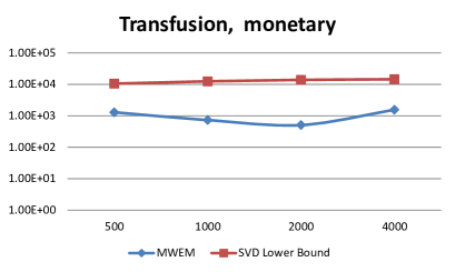
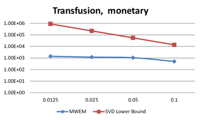
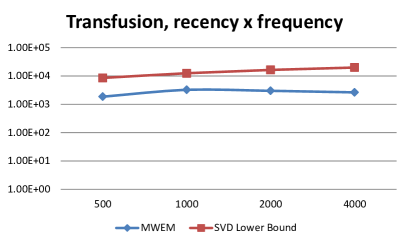
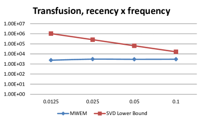
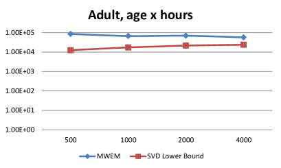
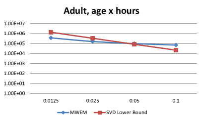
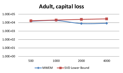
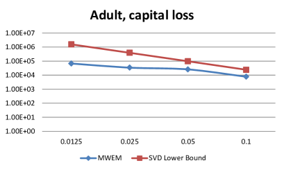
Figure 2: Comparison of MWEM with the SVD lower bound on four data sets. The $y$-axis in each plot represents the average squared error per query. On the left hand side we vary the number of queries from $500$ to $4000$ while keeping $\varepsilon=0.1$ fixed. On the right hand side, we vary $\varepsilon$ from $0.0125$ to $0.1$ while keeping the number of queries $|Q|=2000$ fixed. We report the average over $5$ independent repetitions of the experiment. On each data set for sufficiently small $\varepsilon$ the error achieved by our algorithm is lower than the SVD bound.

3.1 Range Queries

A range query over a domain $D=\{1,\dots,N\}$ is a counting query specified by the indicator function of an interval $I\subseteq D.$ The concept extends naturally to multi-dimensional domains $D=D_{1}\times\dots D_{d}$ where $D_{i}=\{1,\dots,N_{i}\}.$ Here, a range query is defined by the indicator function of a cross product of intervals: the function value is $1$ if and only if each coordinate lies in the associated interval.

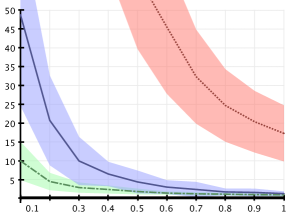
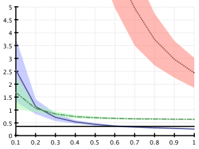
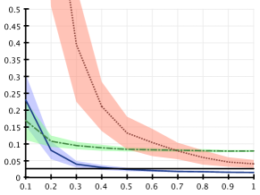
Figure 3: Curves describing the behavior of algorithms on the mildew, rochdale, and czech datasets, respectively. The x-axis is the value of epsilon guaranteed, and the y-axis is the relative entropy between the produced distribution and actual dataset. The lines represent averages across 100 runs, and the corresponding shaded areas one standard deviation in each direction. Red (dashed) represents the modified Barak et al. algorithm, green (dot-dashed) represents unoptimized MWEM, and blue (solid) represents the optimized version thereof. The solid black horizontal line is the stated relative entropy values from Fienberg et al.

Differentially private algorithms for range queries were specifically considered by [2, 25, 17, 18, 19, 20, 21]. As noted in [19, 21], all previously implemented algorithms for range queries can be seen as instances of the matrix mechanism of [18]. Moreover, [19, 21] show a lower bound on the total squared error achieved by the matrix mechanism in terms of the singular values of a matrix associated with the set of queries. We refer to this bound as the SVD bound.

We empirically evaluate MWEM for range queries on several real-world data sets. Specifically, we consider (a) the “capital loss” attribute of the Adult data set [14] corresponding to a domain of size $4357,$ (b) the combined “age” and “hours” attributes of the Adult data set corresponding to a domain of size $91\times 25$, (c) the combined “recency” and “frequency” attributes of the Blood Transfusion data set [14, 26] corresponding to a domain of size $80\times 55$, and (d) the “monetary” attribute of the Blood Transfusion data set corresponding to a domain of size $1251.$ We chose these data sets as they feature numerical attributes of suitable size.

3.1.1 Experimental results

In Figure 2, we compare the performance of MWEM on sets of randomly chosen range queries against the SVD lower bound proved by [19, 21], (1) varying the numbers of queries ($|Q|$) while keeping $\varepsilon$ fixed, and (2) varying $\varepsilon$ while keeping the number of queries fixed. We chose $T\in\{10,12,14,16\}$ for our experiments and reported the values for the best setting of $T$ in each case. The reported numbers are averages of $5$ independent repetitions of the same experiment. We report the total squared error and SVD bound normalized by the total number of queries.

In all four cases we observe that the error achieved by MWEM is lower than the SVD lower bound on the matrix mechanism, for sufficiently small privacy parameter $\varepsilon.$ The improvement against the SVD bound is often by more than an order of magnitude and sometimes by up to three orders of magnitude. Moreover, the privacy guarantee achieved by our algorithm is $(\varepsilon,0)$-differential privacy whereas the SVD lower bound holds for algorithms achieving the strictly weaker guarantee of $(\varepsilon,\delta)$-differential privacy with $\delta>0.$ The SVD bound depends on $\delta$; in our experiments we fixed $\delta=1/n$ when instantiating the SVD bound, as any larger value of $\delta$ would permit exact release of individual records.

3.2 Contingency Tables

A contingency table can be thought of as a table of records over $d$ binary attributes, and the $k$-way marginals of a contingency table correspond to the $d\choose k$ possible choices of $k$ attributes, where each marginal is represented by the $2^{k}$ counts of the records with each possible setting of attributes. Marginals of contingency tables exhibit interesting correlations between queries, and have a significant role in the practice of official statistics. When statistical inference is performed over contingency tables, data analysts seek sets of low-dimensional marginals (i.e., containing relatively few attributes at a time) that fit the data well. Our goal in releasing a differentially private contingency table is to preserve these low-dimensional marginals.

In previous work, Barak et al. [1] describe an approach to differentially private contingency table release through the Hadamard transformation. If we view a contingency table as vector with the coordinates ordered lexicographically by (binary) attribute settings, the Hadamard transformation corresponds to multiplication by the Hadamard matrix, defined recursively as

$$H_{n+1}=\left[\begin{array}[]{rr}H_{n}&H_{n}\\ H_{n}&-H_{n}\end{array}\right]\,,\qquad H_{1}=[1]\,.$$

Importantly, all $k$-dimensional marginals can be exactly recovered by examination of relatively few entries in the transformed vector (roughly $d\choose k$ out of $2^{d}$). Each of these entries corresponds to a set of at most $k$ out of $d$ attributes, where the entry is the difference between the number of records with an even number of bits set and the number of records with an odd number of bits set. Rather than explain which entries to combine and how (details can be found in Barak et al. [1]) we simply take the measurements as our query set, thereby ensuring that our output will respect them. The marginals can then be derived directly from the dataset we produce. Note that we do not need to specify the relationship between the measurements we take and the quantities of interest; we only need that the relationships exist. This is helpful in settings where the dependence is complicated or inexact.

3.2.1 Experimental Setup

In this section, we consider several datasets used in the statistical literature. The datasets, detailed in Table 1, range from small (70 records) to substantial (21k records).

	records	attributes	non-zero / total cells
mildew	70	6	22 / 64
czech	1841	6	63 / 64
rochdale	665	8	91 / 256
nltcs	21574	16	3152 / 65536

Table 1: Details of the four datasets we consider.

We evaluate our approximate dataset with the truth using relative entropy, also known as the Kullback-Leibler (or KL) divergence. Formally, the relative entropy between our two distributions ($A/n$ and $B/n$) is

$$RE(B||A)=\sum_{x\in D}B(x)\log(B(x)/A(x))/n\;.$$

This measurement has appealing properties for statistical inference, and is used in previous statistical work on the problem. Our experiments are intended both to compare our approach to the prior work of Barak et al. [1] as well as to evaluate it in absolute terms. For the purposes of our experiments, Barak et al. is represented by the approach that takes all low order measurements with a uniform level of accuracy and applies Multiplicative Weights (the approach in [1] involved a linear programming step instead of Multiplicative Weights, which we have found only hurts its performance with respect to relative entropy). For the absolute comparison, we invoke the work of Fienberg et al. [13] on several of these datasets where they report absolute numbers for quality of fit (in terms of relative entropy) without privacy constraints, but at a certain level of statistical generality (that is, they do not want to overfit).

We consider both a standard application of MWEM, and one in which we use two optimizations described in Section 2.3.3: re-execution of measured queries and initialization using a histogram over the domain $D$ of records.

3.2.2 Experimental Results

We first evaluate MWEM on several small datasets in common use by statisticians. Our findings here are fairly uniform across the datasets: the ability to measure only those queries that are informative about the dataset results in substantial savings over taking all possible measurements. We evaluate both our theoretically pure algorithm and its heuristic improvement as discussed in the previous section, against a modified version of the algorithm of Barak et al. [1] (improved by integrating the Multiplicative Weights of Hardt-Rothblum [16]), and the accepted “good” non-private relative entropy values from Fienberg et al. [13]. The trade-off between relative entropy and $\varepsilon$ for three datasets appears in Figure 3. In each case, we see that we noticeably improve on the algorithm of Barak et al., and in many cases our heuristic approach matches the good non-private values of [13], indicating that we can approach levels of accuracy at the limit of statistical validity.

We also consider a larger dataset, the National Long-Term Care Study (NLTCS), in Figure 4. This dataset contains orders of magnitudes more records, and has 16 binary attributes. For our initial settings, maintaining all three-way marginals, we see similar behavior as above: the ability to choose the measurements that are important allows substantially higher accuracy on those that matter. However, we see that the algorithm of Barak et al. [1] is substantially more competitive in the regime where we are interested in querying all two-dimensional marginals, rather than the default three we have been using. In this case, for values of epsilon at least $0.1$, it seems that there is enough signal present to simply measure all corresponding entries of the Hadamard transform; each is sufficiently informative that measuring substantially fewer at higher accuracy imparts less information, rather than more.

For every dataset and query set, there is some sufficiently high epsilon level where the judicious selection of queries is no longer required. In such regimes, the approach we present in this paper does not provide an improvement over more naive approaches. The impact of our approach returns if we increase the dimension of the marginal that must be preserved (dramatically increasing the number of measurements Barak et al. would take) or if we decrease $\varepsilon$ to a level such that the majority of two-way measurements are not above the noise level, both of which are demonstrated in Figure 4. However, the analyst’s goal should be to get the right output for the analysis task at hand, under the supplied privacy constraints. In some cases this may not require our advanced query selection.

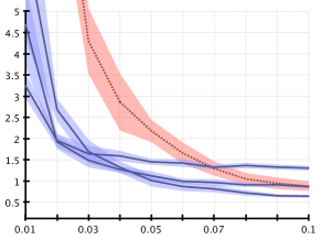
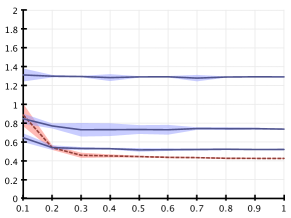
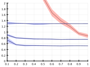
Figure 4: Curves comparing our approach with that of Barak et al. on the National Long Term Care Survey. The red (dashed) curve represents Barak et al, and the multiple blue (solid) curves represent MWEM, with 20, 30, and 40 queries (top to bottom, respectively). From left to right, the first two figures correspond to degree 2 marginals, and the third to degree 3 marginals. As before, the x-axis is the value of epsilon guaranteed, and the y-axis is the relative entropy between the produced distribution and actual dataset. The lines represent averages across only 10 runs, owing to the high complexity of Barak et al. on this many-attributed dataset, and the corresponding shaded areas one standard deviation in each direction.

3.3 Data Cubes

We now change our terminology and objectives, shifting our view of contingency tables to one of datacubes. The two concepts are interchangeable, a contingency table corresponding to the datacube, and a marginal corresponding to its cuboids. However, the datasets studied and the metrics applied are different. We focus on the restriction of the Adult dataset [14] to its eight categorical attributes, as done in [3], and evaluate our approximations using average error within a cuboid, also as done in [3].

Although MWEM is defined with respect to a single query at a time, it generalizes to sets of counting queries, as reflected in a cuboid. The Exponential Mechanism can select a cuboid to measure using a quality score function summing the absolute values of the errors within the cells of the cuboid. We also (heuristically) subtract the number of cells from the score of a cuboid to bias the selection away from cuboids with many cells, which would collect Laplace error in each cell. This subtraction does not affect privacy properties. An entire cuboid can be measured with a single differentially private query, as any record contributes to at most one cell (this is a generalization of the Laplace Mechanism to multiple dimensions, from [5]). Finally, Multiplicative Weights works unmodified, increasing and decreasing weights based on the over- or under-estimation of the count to which the record contributes.

3.3.1 Experimental Results

We apply MWEM to the Adult dataset in several ways: restricting our computation to 2-way cuboids, 3-way cuboids, and with no restriction. As it turns out, the latter two are identical, in that the higher order cuboids have too many cells to be appealing to the algorithm, and are ignored by MWEM. In fact, the 3-way cuboid experiment used only one 3-way cuboid, albeit a very helpful one. We plot the maximum cuboid error and average cuboid error in Figure 5. Comparing our final 3-way measurements ($\max=138.71$ and $\textrm{avg}=13.21$) to the $\varepsilon=1$ reading in Figure 3 of [3], the maximum error appears comparable to their best result, whereas the average error appears approximately four times lower than their best result. Of note, our results are achieved by a single algorithm, whereas the best results for maximum and average error in [3] are achieved by different algorithms, each designed to optimize one specific metric.

4 A Scalable Implementation

The implementation of MWEM used in the previous experiments quite literally maintains a distribution $A_{i}$ over the elements of the universe $D$. As the number of attributes grows, the universe $D$ grows exponentially, and it can quickly become infeasible to track the distribution explicitly. In this section, we consider a scalable implementation with essentially no memory footprint, whose running time is in the worst case proportional to $|D|$, but which for many classes of simple datasets remains linear in the number of attributes.

First, recall that the heart of MWEM is to use Multiplicative Weights to maintain a distribution $A_{i}$ over $D$ that is then used in the Exponential Mechanism to select queries poorly approximated by the current distribution. From the definition of the Multiplicative Weights distribution, we see that the weight $A_{i}(x)$ can be determined from the history $H_{i}=\{(q_{j},m_{j}):j\leq i\}$:

$$A_{i}(x)\propto\exp\left(\sum_{j\leq i}q_{j}(x)\times(m_{j}-q_{j}(A_{j-1}))/2n\right)\,.$$

We explicitly record the scaling factors $l_{j}=m_{j}-q_{j}(A_{j-1})$ as part of the history $H_{i}=\{(q_{j},m_{j},l_{j}):j\leq i\}$, to remove the dependence on prior $A_{j}$. If one is willing to iterate over all $x\in D$, one can evaluate each query $q(A_{i})$ using only this history. Additionally, the summation over $x\in D$ is extremely parallelizable, and distributes easily across multiple cores and computers. While the implicit representation of the distribution $A_{i}$ in terms of the history represents a substantial savings in memory footprint, $D$ can still be exponential in the number of attributes, and even a large cluster is quickly overwhelmed by the required computation.

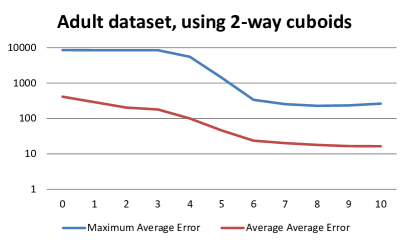
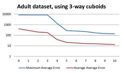
Figure 5: Maximum and average error across all 256 cuboids as 10 steps of $\varepsilon=1$ MWEM proceed, where the cuboid error is taken to be the average over its cells of the absolute values of the cell’s error.

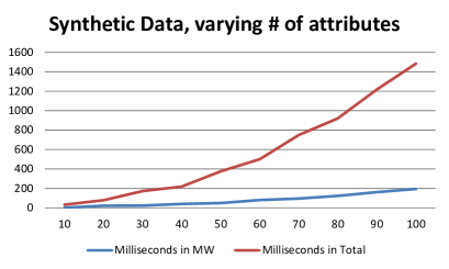
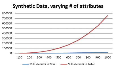
Figure 6: Milliseconds spent in MWEM logic, and Milliseconds spent in total, with the latter containing time spent evaluating queries against the source dataset, the $q_{i}(B)$ evaluations. Even for 1000 binary attributes, we spend only 19 seconds in MWEM.

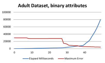
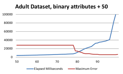
Figure 7: Elapsed milliseconds (increasing) and maximum error (decreasing) as iterations of MWEM proceed. In the second figure, we have added 50 attributes and not plotted the first 50 measurements. The shapes of the curves are very similar, demonstrating how MWEM is capable of ignoring irrelevant attributes. The second experiment takes more time due to the larger number of queries: (77 choose 3) versus (27 choose 3).

Fortunately, the distribution we maintain has additional properties we can exploit. The domain $D$ is often the product of many attributes. If we partition these attributes into disjoint parts $D_{1},D_{2},\ldots D_{k}$ so that no query in $H_{i}$ involves attributes from more than one part, then the distribution produced by Multiplicative Weights is a product distribution over $D_{1}\times D_{2}\times\ldots D_{k}$.

$$\sum_{x\in D_{1}\times D_{2}\times\ldots D_{k}}q(x)\times A_{i}(x)=\prod_{1\leq j\leq k}\left(\sum_{x_{j}\in D_{j}}q(x_{j})\times A^{j}_{i}(x_{j})\right)\;.$$

where $A_{i}^{j}$ is a mini Multiplicative Weights over attributes in part $D_{j}$, using only the relevant queries from $H_{i}$.

Importantly, each of the summations above is now over a potentially much smaller space, reducing the running time from exponential in the number of attributes in $D$ to the sum of the exponentials in the attributes in the $D_{j}$, each of which can be quite small. In the worst case, all attributes are entangled and we have improved nothing, but for many realistic datasets independent or irrelevant groups of attributes exist, and come at essentially no cost in terms of running time or memory footprint.

4.1 Scaling Evaluation

We now experimentally evaluate the scaling performance of this optimized algorithm on synthetic datasets chosen to highlight its behavior, and on one real-world dataset in an attempt to sketch how it might behave in practice. Our experiments are conducted on an AMD Opteror ‘Magny-Cours’ with 48 processors at 1.9GHz.

Our first experiment is run on a synthetic dataset containing 100,000 records, over a number of binary attributes varying from 10 to 100, and then from 100 to 1000. We chose to set each attribute with probability $p=0.1$, and $T$ equal to the number of attributes. In Figure 6 we see both the total running time and the time spent in MWEM. The running time is almost exclusively dominated by the evaluation of the queries against the private data, $B$, and the time spent in the factorized implementation of MWEM is essentially negligible. Each query must be evaluated against $B$, and despite a 48x speed-up the 100,000 records take more time to process than the factored MWEM, in which all attributes are in independent components.

Our second experiment evaluates the performance of our factorized implementation on a binarized form of the Adult dataset where each attribute is replaced by a number of binary attributes equal to the logarithm of its range. This results in 27 binary attributes (from 8 discrete attributes). In Figure 7 we plot the elapsed running time in milliseconds as a function of the index $i$ of the MWEM computation (increasing), and the maximum error across all queries (decreasing). We also repeat the experiment after adding 50 new binary attributes whose values are set with probability $0.1$, to demonstrate that our approach successfully ignores irrelevant attributes, both in terms of running time and maximum error. In this experiment, MWEM is a significant contributor to the running time. The absolute running time increases noticeably as the set of measurements increases in complexity, but until that point each measurement and round of updates takes less than a second. The actual MWEM complexity stays below $|D_{1}|=2^{27}$ and at no point does it approach $|D_{2}|=2^{77}$.

We can perform the corresponding experiment on the original eight categorical attributes of Adult, but with so few attributes the $D_{j}$ are too quickly conflated to give an improvement. We expect the improvement would be more noticeable on a larger dataset.

5 Conclusions

We introduced MWEM, a simple algorithm for releasing data maintaining a high fidelity to the protected source data, as well as differential privacy with respect to the records. The approach builds upon the Multiplicative Weights approach of [16, 15], by introducing the Exponential Mechanism [22] as a more judicious approach to determining which measurements to take. The theoretical analysis matches previous work in the area, and experimentally we have evidence that for many interesting settings, MWEM represents a substantial improvement over existing techniques.

As well as improving on experimental error, the algorithm is both simple to implement and simple to use. An analyst does not require a complicated mathematical understanding of the nature of the queries (as the community has for linear algebra [19] and the Hadamard transform [1]), but rather only needs to enumerate those measurements that should be preserved. We hope that this generality leads to a broader class of high fidelity differentially-private data releases across a variety of data domains.

Appendix A Appendix: Proof of Theorem 2.3

The proof of Theorem 2.3 is broken into two parts. First, we argue that across all $T$ iterations, the queries $q_{i}$ selected by the Exponential Mechanism are nearly optimal, and the errors introduced into $m_{i}$ by the Laplace Mechanism are small. We then apply the potential function analysis of Hardt and Rothblum [16] to show that the maximum approximation error for any query cannot be too large.

Using the shorthand $\mathrm{maxerr}_{i}\stackrel{{\scriptstyle\small\mathrm{def}}}{{=}}\max_{j}|q_{j}(A_{i-1})-q_{j}(B)|$ and $\mathrm{adderr}\stackrel{{\scriptstyle\small\mathrm{def}}}{{=}}2T\log|Q|/\varepsilon$, we first claim that with high probability the Exponential Mechanism and Laplace Mechanism give nearly optimal results.

Lemma A.1.

With probability at least $1-2T/|Q|^{c}$, for any $c\geq 0$, for all $1\leq i\leq T$, we have that both

$$|q_{i}(A_{i-1})-q_{i}(B)| \geq \mathrm{maxerr}_{i}-(2c+2)\times\mathrm{adderr}$$

$$|m_{i}-q_{i}(B)| \leq c\times\mathrm{adderr}\;.$$

Proof A.2.

The probability the Exponential Mechanism with parameter $\varepsilon/2T$ selects a query with quality score at least $r$ less than the optimal (meaning the query on which $A_{i-1}$ disagrees the most with $B$) is bounded by

$$\operatorname*{\mathbb{P}r}[|q_{i}(A_{i-1})-q_{i}(B)|<\mathrm{maxerr}_{i}-r]\leq|Q|\times\exp(-\varepsilon r/4T).$$

If we take $r=(2c+2)\times 2T\log|Q|/\varepsilon$ the probability is at most $1/|Q|^{c}$ for each iteration.

By the definition of the Laplace distribution,

$$\operatorname*{\mathbb{P}r}[|\textrm{Laplace}(2T/\varepsilon)|>r]\leq\exp(-r\times\varepsilon/2T)\;.$$

Taking $r=c\times 2T\log|Q|/\varepsilon$ bounds the probability by at most $1/|Q|^{c}$ for each iteration.

Taking a union bound over the $2T$ events, we arrive at a failure probability of at most $2T/|Q|^{c}$.

We next argue that MWEM improves its approximation in each round where $q_{i}(A)-q_{i}(B)$ has large magnitude. To capture the improvement, we use the relative entropy again:

$$\Psi_{i}=\sum_{x\in D}B(x)\log(B(x)/A_{i}(x))/n\;.$$

The following two properties follow from non-negativity of entropy, and Jensen’s Inequality:

Fact 1.

$\Psi_{i}\geq 0$

Fact 2.

$\Psi_{0}\leq\log|D|$

We now show that the relative entropy decreases in each round by an amount reflecting the error $q_{i}$ exposes between $A_{i-1}$ and $B$, less the error in our measurement of $q_{i}(B)$.

Lemma A.3.

For each round $i\leq T$,

$$\Psi_{i-1}-\Psi_{i}\geq\left(\frac{q_{i}(A_{i-1})-q_{i}(B)}{2n}\right)^{2}-\left(\frac{m_{i}-q_{i}(B)}{2n}\right)^{2}\;.$$

Proof A.4.

We start by noting that

$$\Psi_{i-1}-\Psi_{i}=\sum_{x\in D}B(x)\log\left(\frac{A_{i}(x)}{A_{i-1}(x)}\right)/n\;.$$

The ratio $A_{i}(x)/A_{i-1}(x)$ can be written as $\exp(q_{i}(x)\eta_{i})/\beta_{i}$, where $\eta_{i}=(m_{i}-q_{i}(A_{i-1}))/2n$ and $\beta_{i}$ is the factor required to renormalize in round $i$. Using this notation,

$$\Psi_{i-1}-\Psi_{i} = \eta_{i}q_{i}(B)/n-\log\beta_{i}\;.$$

The required renormalization $\beta_{i}$ equals

$$\beta_{i}=\sum_{x\in D}\exp(q_{i}(x)\eta_{i})A_{i-1}(x)/n\;.$$

Using $\exp(x)\leq 1+x+x^{2}$ for $|x|\leq 1$, and that $|q_{i}(x)\eta_{i}|\leq 1$,

$$\beta_{i}\leq\sum_{x\in D}(1+q_{i}(x)\eta_{i}+q_{i}(x)^{2}\eta_{i}^{2})A_{i-1}(x)/n\;.$$

As $q_{i}(x)^{2}\leq 1$, by assumption on all $q_{i}\in Q$, we have

$$\beta_{i} \leq \sum_{x\in D}(1+q_{i}(x)\eta_{i}+\eta_{i}^{2})A_{i-1}(x)/n$$

$$= 1+\eta_{i}q_{i}(A_{i-1})/n+\eta_{i}^{2}\;.$$

Introducing this bound on $\beta_{i}$ into our equality for $\Psi_{i-1}-\Psi_{i}$, and using $\log(1+x)\leq x$, we get

$$\Psi_{i-1}-\Psi_{i}\geq\eta_{i}(q_{i}(B)-q_{i}(A_{i-1}))/n-\eta_{i}^{2}\;.$$

After reintroducing the definition of $\eta_{i}$ and simplifying, this bound results in the statement of the lemma.

With these two lemmas we are now prepared to prove Theorem 2.3, bounding the maximum error $|q(A)-q(B)|$.

Proof A.5 ((of Theorem 2.3)).

We start by noting that the quantity of interest, the maximum over queries $q$ of the error between $q(A)$ and $q(B)$, can be rewritten and bounded by:

$$\max_{q\in Q}|q(A)-q(B)| = \max_{q\in Q}|q(\mathop{\textrm{avg}}_{i\leq T}A_{i})-q(B)|$$

$$\leq \max_{q\in Q}\mathop{\textrm{avg}}_{i\leq T}|q(A_{i})-q(B)|$$

$$\leq \mathop{\textrm{avg}}_{i\leq T}\mathrm{maxerr}_{i}\;.$$

At this point we invoke Lemma A.1 with $c=1$ so that with probability at least $1-2T/|Q|$ we have for $i\leq T$ both

$$\mathrm{maxerr}_{i} \leq |q_{i}(A_{i-1})-q_{i}(B)|+4\times\mathrm{adderr}\;,$$

$$|m_{i}-q_{i}(B)| \leq \mathrm{adderr}\;.$$

Combining these bounds with those of Lemma A.3 gives

$$\mathrm{maxerr}_{i} \leq \left(4n^{2}(\Psi_{i-1}-\Psi_{i})+\mathrm{adderr}^{2}\right)^{1/2}+4\times\mathrm{adderr}\;.$$

We now average over $i\leq T$, and apply Cauchy-Schwarz, specifically that $\mathop{\textrm{avg}}_{i}x_{i}^{1/2}\leq(\mathop{\textrm{avg}}_{i}x_{i})^{1/2}$, giving

$$\mathop{\textrm{avg}}_{i\leq T}\;\mathrm{maxerr}_{i} \leq \left(4n^{2}\mathop{\textrm{avg}}_{i}(\Psi_{i-1}-\Psi_{i})+\mathrm{adderr}^{2}\right)^{1/2}$$

$$+\;4\times\mathrm{adderr}\;.$$

The average $\mathop{\textrm{avg}}_{i}(\Psi_{i-1}-\Psi_{i})$ telescopes to $(\Psi_{0}-\Psi_{T})/T$, which Facts 1 and 2 bound by $\log(|D|)/T$, giving

$$\mathop{\textrm{avg}}_{i\leq T}\;\mathrm{maxerr}_{i}\leq\left(4n^{2}\log(|D|)/T+\mathrm{adderr}^{2}\right)^{1/2}+\;4\times\mathrm{adderr}\;.$$

Finally, as $\sqrt{a+b}\leq\sqrt{a}+\sqrt{b}$, we derive

$$\mathop{\textrm{avg}}_{i\leq T}\;\mathrm{maxerr}_{i} \leq 2n(\log(|D|)/T)^{1/2}+5\times\mathrm{adderr}\;.$$

If we substitute $2T\log|Q|/\varepsilon$ for adderr we get the bound in the statement of the theorem. Replacing the factor of $5$ by $(3c+2)$ generalizes the result to hold with probability $1-2T/|Q|^{c}$ for arbitrary $c>0$.

double[] MultiplicativeWeightsViaExponentialMechanism(double[] B, Func<int, double>[] Q, int T, double eps)
{
    var n = (double) B.Sum();                                     // should be taken privately, we ignore
    var A = Enumerable.Repeat(n / B.Length, B.Length).ToArray();  // approx dataset, initially uniform
    var measurements = new Dictionary<int, double>();             // records (qi, mi) measurement pairs
    var random = new Random();                                    // RNG used all over the place

    for (int i = 0; i < T; i++)
    {
        // determine a new query to measure, rejecting prior queries
        var qi = random.ExponentialMechanism(B, A, Q, eps / (2 * T));
        while (measurements.ContainsKey(qi))
            qi = random.ExponentialMechanism(B, A, Q, eps / (2 * T));

        // measure the query, and add it to our collection of measurements
        measurements.Add(qi, Q[qi].Evaluate(B) + random.Laplace((2 * T) / eps));

        // improve the approximation using poorly fit measurements
        A.MultiplicativeWeights(Q, measurements);
    }

    return A;
}

int ExponentialMechanism(this Random random, double[] B, double[] A, Func<int, double>[] Q, double eps)
{
    var errors = new double[Q.Length];
    for (int i = 0; i < errors.Length; i++)
        errors[i] = eps * Math.Abs(Q[i].Evaluate(B) - Q[i].Evaluate(A)) / 2.0;

    var maximum = errors.Max();
    for (int i = 0; i < errors.Length; i++)
        errors[i] = Math.Exp(errors[i] - maximum);

    var uniform = errors.Sum() * random.NextDouble();
    for (int i = 0; i < errors.Length; i++)
    {
        uniform -= errors[i];
        if (uniform <= 0.0)
            return i;
    }

    return errors.Length - 1;
}

double Laplace(this Random random, double sigma)
{
    return sigma * Math.Log(random.NextDouble()) * (random.Next(2) == 0 ? -1 : +1);
}

void MultiplicativeWeights(this double[] A, Func<int, double>[] Q, Dictionary<int, double> measurements)
{
    var total = A.Sum();

    for (int iteration = 0; iteration < 100; iteration++)
    {
        foreach (var qi in measurements.Keys)
        {
            var error = measurements[qi] - Q[qi].Evaluate(A);
            for (int i = 0; i < A.Length; i++)
                A[i] *= Math.Exp(Q[qi](i) * error / (2.0 * total));

            var count = A.Sum();
            for (int i = 0; i < A.Length; i++)
                A[i] *= total / count;
        }
    }
}

double Evaluate(this Func<int, double> query, double[] collection)
{
    return Enumerable.Range(0, collection.Length).Sum(i => query(i) * collection[i]);
}

Figure 8: Full source code for a reference implementation of MWEM.

References

- [1] B. Barak, K. Chaudhuri, C. Dwork, S. Kale, F. McSherry, and K. Talwar. Privacy, accuracy, and consistency too: a holistic solution to contingency table release. In PODS, 2007.
- [2] Avrim Blum, Katrina Ligett, and Aaron Roth. A learning theory approach to non-interactive database privacy. In STOC, 2008.
- [3] Bolin Ding, Marianne Winslett, Jiawei Han, and Zhenhui Li. Differentially private data cubes: optimizing noise sources and consistency. In SIGMOD, 2011.
- [4] I. Dinur and K. Nissim. Revealing information while preserving privacy. In PODS, 2003.
- [5] C. Dwork, F. McSherry, K. Nissim, and A. Smith. Calibrating noise to sensitivity in private data analysis. In TCC, 2006.
- [6] C. Dwork, M. Naor, O. Reingold, G.N. Rothblum, and S. Vadhan. On the complexity of differentially private data release: efficient algorithms and hardness results. In STOC, 2009.
- [7] C. Dwork and S. Yekhanin. New Efficient Attacks on Statistical Disclosure Control Mechanisms. In CRYPTO, 2008.
- [8] Cynthia Dwork. The differential privacy frontier (extended abstract). In TCC, 2009.
- [9] Cynthia Dwork. The promise of differential privacy: A tutorial on algorithmic techniques. In FOCS, 2011.
- [10] Cynthia Dwork, Moni Naor, Omer Reingold, Guy N. Rothblum, and Salil P. Vadhan. On the complexity of differentially private data release: efficient algorithms and hardness results. In STOC, 2009.
- [11] Cynthia Dwork and Kobbi Nissim. Privacy-preserving datamining on vertically partitioned databases. In CRYPTO. Springer, 2004.
- [12] Cynthia Dwork, Guy Rothblum, and Salil Vadhan. Boosting and differential privacy. In FOCS, 2010.
- [13] Stephen E. Fienberg, Alessandro Rinaldo, and Xiolin Yang. Differential privacy and the risk-utility tradeoff for multi-dimensional contingency tables. In Privacy in Statistical Databases, 2010.
- [14] A. Frank and A. Asuncion. UCI machine learning repository, 2010.
- [15] Anupam Gupta, Moritz Hardt, Aaron Roth, and Jon Ullman. Privately releasing conjunctions and the statistical query barrier. In STOC, 2011.
- [16] Moritz Hardt and Guy Rothblum. A multiplicative weights mechanism for interactive privacy-preserving data analysis. In FOCS, 2010.
- [17] Michael Hay, Vibhor Rastogi, Gerome Miklau, and Dan Suciu. Boosting the accuracy of differentially-private queries through consistency. In VLDB, 2010.
- [18] C. Li, M. Hay, V. Rastogi, G. Miklau, and A. McGregor. Optimizing linear counting queries under differential privacy. In PODS, 2010.
- [19] Chao Li and Gerome Miklau. Efficient batch query answering under differential privacy. CoRR, abs/1103.1367, 2011.
- [20] Chao Li and Gerome Miklau. An adaptive mechanism for accurate query answering under differential privacy. to appear, PVLDB, 2012.
- [21] Chao Li and Gerome Miklau. Measuring the achievable error of query sets under differential privacy. CoRR, abs/1202.3399v2, 2012.
- [22] Frank McSherry and Kunal Talwar. Mechanism design via differential privacy. In FOCS, 2007.
- [23] Aaron Roth and Tim Roughgarden. The median mechanism: Interactive and efficient privacy with multiple queries. In STOC, 2010.
- [24] Jonathan Ullman and Salil P. Vadhan. PCPs and the hardness of generating private synthetic data. In TCC, 2011.
- [25] Xiaokui Xiao, Guozhang Wang, and Johannes Gehrke. Differential privacy via wavelet transforms. IEEE Transactions on Knowledge and Data Engineering, 23:1200–1214, 2011.
- [26] I-Cheng Yeh, King-Jang Yang, and Tao-Ming Ting. Knowledge discovery on RFM model using Bernoulli sequence. Expert Systems with Applications, 36(3), 2008.