Description of thermal entanglement with the static path plus random phase approximation

Abstract

We discuss the application of the static path plus random phase approximation (SPA+RPA) and the ensuing mean field+RPA treatment to the evaluation of entanglement in composite quantum systems at finite temperature. These methods involve just local diagonalizations and the determination of the generalized collective vibrational frequencies. As illustration, we evaluate the pairwise entanglement in a fully connected XXZ chain of $n$ spins at finite temperature in a transverse magnetic field $b$. It is shown that already the mean field+RPA provides an accurate analytic description of the concurrence below the mean field critical region ($|b|<b_{c}$), exact for large $n$, whereas the full SPA+RPA is able to improve results for finite systems in the critical region. It is proved as well that for $T>0$ weak entanglement also arises when the ground state is separable ($|b|>b_{c}$), with the limit temperature for pairwise entanglement exhibiting quite distinct regimes for $|b|<b_{c}$ and $|b|>b_{c}$.

I Introduction

It is now well recognized that quantum entanglement plays an essential role in both quantum information science NC.00 , where it is considered a resource, as well as in many-body and condensed matter physics, where it provides a new perspective for understanding quantum correlations and critical phenomena ON.02 ; OS.02 ; V.03 ; T.04 . Entanglement denotes those correlations with no classical analogue that can be exhibited by composite quantum systems, which constitute, for instance, the key ingredient in quantum teleportation Be.93 . A pure state of a composite system is entangled if it is not a product state, while a mixed state of such system is entangled when it cannot be written as a convex combination of product states W.89 .

Thermal entanglement ON.02 ; ABV.01 ; Wa.02 ; W.04 ; AK.04 ; CR.04 denotes that of mixed states of the form $\rho(T)\propto\exp[-\beta H]$, where $H$ is the system Hamiltonian and $\beta=1/kT$ the inverse temperature. A complete characterization of thermal entanglement in many component systems is difficult, since, to begin with, there is no simple necessary and sufficient computable criterion for determining if a general mixed state is entangled DPS.04 . Besides, these systems exhibit entanglement at different levels, i.e., between any pair or set of subsystems, starting from that between elementary constituents $i,j$ and ending in that of global partitions RC.05 (which for $T>0$ can no longer be measured through the entropy of a subsystem). Finally, a basic difficulty is the accurate evaluation of $\rho(T)$ and the ensuing reduced densities $\rho_{ij}$. Standard methods like the mean field approximation (MFA), which may provide a correct basic description of thermodynamic observables in some systems, are not suitable for the evaluation of entanglement since they are based on separable (non-entangled) trial densities. In small finite systems fluctuations of the order parameters become important S.72 and the MFA is to be replaced at least with some average over different mean field densities, but such an approach will still fail to describe entanglement as it is essentially based on a convex combination of product densities.

The principal goal of this work is to show the applicability of the static path plus random phase approximation (SPA+RPA) PBB.91 ; AA.97 ; RC.97 ; RCR.98 to the determination of thermal entanglement. The approach is derived from the path integral representation of the partition function obtained with the Hubbard-Stratonovich transformation HS.57 , and has been applied to the description of basic observables in diverse fermionic models of nuclear and condensed matter physics PBB.91 ; AA.97 ; RC.97 ; RCR.98 ; CR.01 ; KK.05 . It takes into account both the large amplitude static fluctuations (SPA) of the mean field order parameters, essential in critical regions of finite systems, together with small amplitude quantum fluctuations (RPA), which may account for most quantum effects if $T$ is not too low and will be responsible for entanglement. It also provides a fully consistent MFA+RPA approach RCR.98 , obtained through the saddle point approximation to the full treatment. Here we will formulate the method for a system of $n$ distinguishable constituents, where it involves in principle just local diagonalizations.

We will employ the formalism to evaluate the thermal pairwise entanglement in a fully connected $XXZ$ chain of $n$ qubits or spins in the presence of a uniform transverse magnetic field $b$. Spin chains constitute an attractive scalable qubit representation for exploring and implementing quantum information processes DV.00 ; DV.98 ; BB.04 and can be realized in diverse physical systems, including those based on quantum dots electron-spins I.99 and Josephson junction arrays MS.01 , where the effective model includes coupling between any two spins. Fully connected symmetric spin models (simplex) have also intrinsic interest, providing a solvable scenario for examining entanglement in systems undergoing phase transitions. In particular, entanglement properties of the fully connected $XX$ and $XY$ model at $T=0$ were thoroughly analyzed in VPM.04 ; V.04 ; V.06 . We will show that the XXZ model exhibits an interesting non trivial behavior at finite temperature, whose main features can be correctly described by the SPA+RPA for moderate finite $n$ and even by the MFA+RPA below the critical region, the latter providing an analytic description which becomes exact for large $n$. The formalism is described in section II while application to the model is discussed in III. Finally, conclusions are drawn in IV.

II Formalism

We will consider a composite system described by a Hamiltonian of the form

$$H=H^{0}-\mbox{$\frac{1}{2}$}\sum_{\nu}v_{\nu}(Q^{\nu})^{2}\,,$$ (1)

where $H^{0}$, $Q^{\nu}$ are linear combinations of local operators, i.e., $H^{0}=\sum_{i}H^{0}_{i}$, $Q^{\nu}=\sum_{i}Q^{\nu}_{i}$, with $H^{0}_{i}$, $Q^{\nu}_{i}$ acting just on subsystem $i$ ($Q^{\nu}_{i}\equiv I_{1}\otimes\ldots\otimes Q_{i}^{\nu}\otimes\ldots\otimes I_{n}$, with $[Q^{\nu}_{i},Q^{\nu}_{j}]=0$ if $i\neq j$). In a spin chain $Q^{\nu}$ could stand, for instance, for total spin operators or general linear combinations $\sum_{i}\alpha_{i}s^{\nu}_{i}$ of the individual spins $s^{\nu}_{i}$. Any quadratic interaction between subsystems,

$$V=-\mbox{$\frac{1}{2}$}\sum_{i,j,\nu,\nu^{\prime}}O^{\nu}_{i}v^{ij}_{\nu\nu^{\prime}}O^{\nu^{\prime}}_{j}\,,$$ (2)

where $O^{\nu}_{i}$ denote local operators, can be written in the diagonal form (1) (non-unique), after completing squares or diagonalizing the matrix $v_{i\nu,j\nu^{\prime}}\equiv v^{ij}_{\nu\nu^{\prime}}$, with $Q^{\nu}$ suitable linear combinations of the $O^{\nu}_{i}$. We may assume $v_{\nu}>0$ in (1) without loss of generality if antihermitian operators $Q^{\nu}$ are allowed ($v_{\nu}(Q^{\nu})^{2}\rightarrow-v_{\nu}(iQ^{\nu})^{2}$). In what follows we will consider finite Hilbert space dimension.

The Hubbard-Stratonovich transformation allows then to express the partition function $Z={\rm Tr}\exp[-\beta H]$ as the path integral HS.57

$$Z = \int\!D[x]\,{\rm Tr}\,\hat{T}\exp\{-\!\int_{0}^{\beta}\!\!d\tau[\sum_{\nu}\frac{x_{\nu}^{2}(\tau)}{2v_{\nu}}+h[x(\tau)]\}\,,$$ (3)

$$h(x) = \sum_{i}h_{i}(x),\;\;\;h_{i}(x)=H^{0}_{i}-\sum_{\nu}x_{\nu}Q^{\nu}_{i}\,,$$ (4)

where $\hat{T}$ denotes time ordering and the normalization $\int\!D[x]\exp[-\!\int_{0}^{\beta}\!d\tau\!\sum_{\nu}\!x_{\nu}^{2}(\tau)/2v_{\nu}]=1$ is assumed. The integrand in (3) is essentially the trace of the imaginary time evolution operator $U[x]$ associated with the path $x(\tau)$ and the linearized Hamiltonian $h[x(\tau)]$, and is here a product operator $\prod_{i}U_{i}[x]$, not necessarily positive. Eq. (3) can be evaluated by means of a Fourier expansion

$$x_{\nu}(\tau)=x_{\nu}+\sum_{n\neq 0}x_{\nu}^{n}e^{i\omega_{n}\tau}\,,\;\;\omega_{n}=2\pi n/\beta\,,$$ (5)

where $x_{\nu}\equiv x_{\nu}^{0}$ are the static coefficients, representing the time average $\langle x_{\nu}(\tau)\rangle_{[0,\beta]}$, with $D[x]\propto\prod_{\nu}dx_{\nu}\prod_{n\neq 0}dx_{\nu}^{n}$.

In the SPA+RPA PBB.91 ; AA.97 ; RC.97 ; RCR.98 (to be denoted for brevity as CSPA (correlated SPA)), the integrals over the static coefficients $x_{\nu}$ are fully preserved, while those over $x_{\nu}^{n}$, $n\neq 0$, are evaluated in the saddle point approximation for each value of the $x_{\nu}$. The aim is to take into account large amplitude static fluctuations, which are particularly relevant in the transitional regions of finite systems, together with small amplitude quantum fluctuations, which should in principle account for most quantum effects if the temperature is not too low. The final result can be expressed as RCR.98

$$Z_{\rm CSPA} = \int_{-\infty}^{\infty}e^{-\beta\sum_{\nu}x_{\nu}^{2}/2v_{\nu}}Z(x)C_{\rm RPA}(x)d(x)\,,$$ (6)

where $d(x)=\prod_{\nu}\sqrt{\beta/(2\pi v_{\nu})}dx_{\nu}$ and

$$Z(x) = {\rm Tr}\exp[-\beta h(x)]=\prod_{i}{\rm tr}\exp[-\beta h_{i}(x)]\,,$$ (7)

$$C_{\rm RPA}(x) = \prod_{n=1}^{\infty}{\rm Det}[\delta_{\nu\nu^{\prime}}+v_{\nu}R_{\nu\nu^{\prime}}(x,i\omega_{n})]^{-1}\,,$$ (8)

$$R_{\nu\nu^{\prime}}(x,\omega) = \sum_{i,k\neq{k^{\prime}}}\frac{\langle k_{i}|Q^{\nu}_{i}|{k^{\prime}}_{i}\rangle\langle{k^{\prime}}_{i}|Q^{\nu^{\prime}}_{i}|k_{i}\rangle(p_{k_{i}}-p_{k^{\prime}_{i}})}{\varepsilon_{k_{i}}-\varepsilon_{k^{\prime}_{i}}+\omega}\,.$$ (9)

with ${\rm tr}$ the local trace, $|k_{i}\rangle$ the running local eigenstates ($h_{i}(x)|k_{i}\rangle=\varepsilon_{k_{i}}|k_{i}\rangle$) and $p_{k_{i}}=e^{-\beta\varepsilon_{k_{i}}}/{\rm tr}\,e^{-\beta h_{i}(x)}$. Eqs. (6)-(9) involve just local diagonalizations. Eq. (8) is the RPA correction, fundamental in the present context, which can be further expressed as AA.97 ; RC.97

$$C_{\rm RPA}(x)=\prod_{\alpha>0}\prod_{n=1}^{\infty}\frac{\lambda_{\alpha}^{2}+\omega_{n}^{2}}{\omega_{\alpha}^{2}+\omega_{n}^{2}}=\prod_{\alpha>0}\frac{\omega_{\alpha}\sinh(\beta\lambda_{\alpha}/2)}{\lambda_{\alpha}\sinh(\beta\omega_{\alpha}/2)}\,,$$ (10)

where $\alpha\equiv(k_{i},k^{\prime}_{i})$ runs over all pairs $k_{i}\neq k^{\prime}_{i}$ ($\alpha>0$ indicating $k_{i}>k^{\prime}_{i}$), $\lambda_{\alpha}\equiv\varepsilon_{k_{i}}-\varepsilon_{k^{\prime}_{i}}$ and $\omega_{\alpha}$ are the running RPA energies, determined as the roots of the equation

$${\rm Det}[\delta_{\nu\nu^{\prime}}+v_{\nu}R_{\nu\nu^{\prime}}(x,\omega)]=0\,.$$ (11)

They come in pairs of opposite sign and can also be obtained as the eigenvalues of the matrix

$$A_{\alpha\alpha^{\prime}}(x)=\lambda_{\alpha}\delta_{\alpha\alpha^{\prime}}+p_{\alpha}\sum_{\nu}v_{\nu}Q^{\nu}_{-\alpha}Q^{\nu}_{\alpha^{\prime}}\,,$$ (12)

where $p_{\alpha}\equiv p_{k_{i}}-p_{k^{\prime}_{i}}$, $Q^{\nu}_{\alpha}\equiv\langle k_{i}|Q^{\nu}_{i}|k^{\prime}_{i}\rangle$. Eq. (6) can be applied provided $C_{\rm RPA}(x)>0$, which implies $\omega_{\alpha}^{2}+\omega_{1}^{2}>0$ $\forall\,\alpha,x$. Since the lowest RPA energies $\omega_{\alpha}$ may become imaginary or complex for $x$ away from the stable mean field solution (see below), the previous condition sets up a breakdown temperature $T^{*}$, normally low, such that Eq. (6) is applicable for $T>T^{*}$. Setting $C_{\rm RPA}(x)=1$ in (6) leads to the plain SPA S.72 , which, although significantly improving the MFA in critical regions, is unable to describe entanglement, as it averages correspond essentially to those of a convex combination of separable densities (for $h(x)$ hermitian).

MFA+RPA. Away from critical regions, we may also apply the saddle point approximation to the static variables $x_{\nu}$. This leads to the MFA+RPA (to be denoted as CMFA), given by RCR.98

$$Z_{\rm CMFA} = e^{-\beta\sum_{\nu}x_{\nu}^{2}/2v_{\nu}}Z(x)C_{0}(x)C_{\rm RPA}(x)\,,$$ (13)

where $x$ is the value which minimizes the “separable” free energy ${\cal F}(x)=\sum_{\nu}x_{\nu}^{2}/2v_{\nu}-T\ln Z(x)$ and is determined by the self-consistent “Hartree” equations

$$x_{\nu}=v_{\nu}\langle Q^{\nu}\rangle_{x}\,,$$ (14)

with $\langle Q^{\nu}\rangle_{x}=\sum_{i,k}p_{k_{i}}\langle k_{i}|Q^{\nu}_{i}|k_{i}\rangle$. $C_{0}(x)$ accounts for the small amplitude static fluctuations and is given by

$$C_{0}(x) = {\rm Det}[v_{\nu}\frac{\partial^{2}{\cal F}(x)}{\partial x_{\nu}\partial x_{\nu^{\prime}}}]^{-1/2}$$ (15)

$$= {\rm Det}[\delta_{\nu\nu^{\prime}}+v_{\nu}(R_{\nu\nu^{\prime}}(x,0)-\sum_{i,k}\langle k_{i}|Q^{\nu}_{i}|k_{i}\rangle\frac{\partial p_{k_{i}}}{\partial x_{\nu^{\prime}}})]^{-1/2}\,,$$

with $\partial p_{k_{i}}/\partial x_{\nu^{\prime}}=\beta p_{k_{i}}\sum_{k^{\prime}_{i}}\langle k^{\prime}_{i}|Q^{\nu^{\prime}}_{i}|k^{\prime}_{i}\rangle(\delta_{kk^{\prime}}-p_{k^{\prime}_{i}})$.

Away from critical points Eq. (13) can be employed right up to $T\rightarrow 0$. Note, however, that if the solution of (14) exhibits a continuous degeneracy (due to a continuous symmetry violation by $h(x)$) the previous approach should be applied just to the intrinsic variables (see sec. III). In this case the lowest RPA energy vanishes at the mean field solution RC.97 ; RCR.98 but Eq. (13) is still applicable, as $C_{\rm RPA}(x)$, Eq. (8), remains finite for $\omega_{\alpha}\rightarrow 0$. Omitting $C_{\rm RPA}(x)$ and $C_{0}(x)$ in (13) leads to the plain MFA, which corresponds to a separable (product) density.

We may then employ Eqs. (6) or (13) to calculate the two-site averages $\langle O_{i}^{\nu}O_{j}^{\nu^{\prime}}\rangle=(2/\beta)\partial\ln Z/\partial v^{ij}_{\nu\nu^{\prime}}$ required to evaluate the reduced density $\rho_{ij}$ and hence a certain monotone or measure of the entanglement between subsystems $i$ and $j$. If not present in the original interaction, we may in principle add the necessary terms in $V$ and set at the end $v^{ij}_{\nu\nu^{\prime}}=0$.

III Application

III.1 Fully connected XXZ Model

We will consider $n$ qubits or spins coupled through a full range $XXZ$ type interaction in the presence of a transverse magnetic field $b$. The Hamiltonian reads

$$H = b\sum_{i=1}^{n}s^{z}_{i}-V\sum_{i\neq j}^{n}[s^{x}_{i}s^{x}_{j}+s^{y}_{i}s^{y}_{j}+(1-\gamma)s^{z}_{i}s^{z}_{j}]$$ (16a)

$$= bS_{z}-V[S_{x}^{2}+S_{y}^{2}+(1-\gamma)S_{z}^{2}]+E_{0}\,,$$ (16b)

where ${\bm{s}_{i}}$ denotes the spin at site $i$ (considered dimensionless), ${\bm{S}}=\sum_{i=1}^{n}{\bm{s}}_{i}$ the total spin, $\gamma$ the anisotropy and $E_{0}=nV(3-\gamma)/4$. It is apparent that $H$ commutes with $S_{z}$ and $S^{2}=S_{x}^{2}+S_{y}^{2}+S_{z}^{2}$, its eigenvalues being

$$E_{SM}=bM-V[S(S+1)-\gamma M^{2}]+E_{0}\,,$$ (17)

where $M=-S,\ldots,S$ and $S=\delta,\ldots,n/2$, with $\delta=0$ $(\mbox{$\frac{1}{2}$})$ for $n$ even (odd). The ensuing partition function is

$$Z={\rm Tr}\exp[-\beta H]=\sum_{S=\delta}^{n/2}Y(S)\sum_{M=-S}^{S}e^{-\beta E_{SM}}\,,$$ (18)

where $Y(S)=(^{\;\;\;\;n}_{n/2-S})-(^{\;\;\;\;\;n}_{n/2-S-1})$, with $Y(\frac{n}{2})=1$, is the multiplicity of states with total spin $S$ and $S_{z}=M$, such that $\sum_{S=\delta}^{n/2}Y(S)(2S+1)=2^{n}$. In what follows we will write

$$V=v/n\,,$$ (19)

such that all intensive energies $E_{SM}/n$ remain finite for $n\rightarrow\infty$ and finite $v$.

We will analyze here the attractive case $v>0$ (and $\gamma\leq 1$), where the ground state has maximum spin $S=n/2$ $\forall$ $b,\gamma$. If $\gamma\leq 0$, the ground state will be fully aligned ($|M|=n/2$) $\forall$ $b\neq 0$ and no ground state entanglement will arise, whereas if $\gamma>0$, the ground state will exhibit as $b$ increases $n$ transitions $M\rightarrow M-1$ at

$$b_{M}=\gamma v(1-2M)/n\,,$$ (20)

where $E_{SM}=E_{S,M-1}$, becoming fully aligned for

$$|b|>b_{c}\equiv\gamma v(1-1/n)\,.$$ (21)

Thus, $b_{c}$ is the limit field for entanglement at $T=0$, as all ground states with $S=n/2$ and $|M|<n/2$ are entangled (see below).

III.2 Exact concurrence

We will examine here the entanglement of a pair of spins $(i,j)$, which is determined by the reduced two-qubit density $\rho_{2}\equiv\rho_{ij}={\rm Tr}_{n-\{i,j\}}\rho(T)$. In the present system $\rho(T)$ is completely symmetric and $\rho_{2}$ will obviously be identical for all pairs $i\neq j$. In the standard basis of $s^{z}_{i},s^{z}_{j}$ eigenstates, it will have the form

$$\rho_{2}=\left(\begin{array}[]{cccc}p_{+}&0&0&0\\ 0&p&\alpha&0\\ 0&\alpha&p&0\\ 0&0&0&p_{-}\end{array}\right)\,,$$ (22)

where $p_{+}+2p+p_{-}=1$ and

$$\begin{array}[]{ccl}p_{\pm}&=&\langle(\mbox{$\frac{1}{2}$}\pm s^{z}_{i})(\mbox{$\frac{1}{2}$}\pm s^{z}_{j})\rangle=\frac{\langle S_{z}^{2}\rangle-n/4}{n(n-1)}+\frac{1}{4}\pm\frac{\langle S_{z}\rangle}{n}\,,\\ \alpha&=&\langle s^{+}_{i}s^{-}_{j}\rangle=\frac{\langle S^{2}\rangle-\langle S_{z}^{2}\rangle-n/2}{n(n-1)}\,,\end{array}$$

with $\langle O\rangle\equiv{\rm Tr}\,\rho\,O$ the thermal average and $s_{i}^{\pm}=s^{x}_{i}\pm is^{y}_{i}$. Hence, $\rho_{2}$ is here completely determined by the three collective averages $\langle S_{z}\rangle$, $\langle S_{z}^{2}\rangle$ and $\langle S^{2}\rangle$, which can be directly derived from Eq. (18) as (we set $k=1$)

$$\begin{array}[]{l}\langle S_{z}\rangle=-T\frac{\partial\ln Z}{\partial b}\,,\;\;\;\;\;\;\langle S_{z}^{2}\rangle=T^{2}\frac{\partial^{2}\ln Z}{\partial b^{2}}+\langle S_{z}\rangle^{2}\\ \langle S^{2}\rangle=nT\frac{\partial\ln Z}{\partial v}+\gamma\langle S_{z}^{2}\rangle+\frac{n(3-\gamma)}{4}\end{array}\,.$$ (23)

We may equivalently use $\langle S_{z}^{2}\rangle=(nT/v)\partial\ln Z/\partial\gamma$.

As a measure of pairwise entanglement we will employ the concurrence $C$ W.98 , which for a general two component system can be defined as the minimum, over all representations $\rho_{ij}=\sum_{\nu}q_{\nu}|\Psi_{\nu}\rangle\langle\Psi_{\nu}|$, of $\sum_{\nu}q_{\nu}C(|\Psi^{\nu}\rangle)$, with $C(|\Psi^{\nu}\rangle)=\sqrt{2[1-{\rm tr}(\rho^{\nu}_{i})^{2}]}$ the square root of the linear entropy of any of the subsystems RC.03 . The entanglement of formation Be.96 is similarly defined but with $C(|\Psi^{\nu}\rangle)$ replaced by the standard entropy $-{\rm Tr}\rho^{\nu}_{i}\log_{2}\rho^{\nu}_{i}$.

For a two qubit system, $C$ can be explicitly computed as W.98 $C=[2\lambda-{\rm tr}R,0]_{+}$, where $[u]_{+}\equiv\mbox{$\frac{1}{2}$}(u+|u|)/2$ and $\lambda$ is the largest eigenvalue of $R=[\sqrt{\rho_{2}}\tilde{\rho}_{2}\sqrt{\rho_{2}}]^{1/2}$, with $\tilde{\rho}_{2}=4^{2}s^{y}_{i}s^{y}_{j}\rho_{2}^{*}s^{y}_{j}s^{y}_{i}$ the spin flipped density. The entanglement of formation becomes then just an increasing function of $C$ (given by $E=-\sum_{\nu=\pm}q_{\nu}\log_{2}q_{\nu}$, with $q_{\pm}=(1\pm\sqrt{1-C^{2}})/2$), with $E=C=0$ (1) for a separable (maximally entangled) pair.

In the present system we then obtain

$$C = 2[\,|\alpha|-\sqrt{p_{+}p_{-}}\,]_{+}$$ (24)

$$= \frac{2}{n}[\frac{|\langle S^{2}\rangle-\langle S_{z}^{2}\rangle-\frac{n}{2}|}{n-1}-\sqrt{(\frac{\langle S_{z}^{2}\rangle+\frac{n(n-2)}{4}}{n-1})^{2}-\langle S_{z}\rangle^{2}}]_{+}$$ (25)

so that $\rho_{2}$ will be entangled if and only if $|\alpha|>\sqrt{p_{+}p_{-}}$, a condition which directly follows from Peres criterion P.96 . In (25) $2/n$ is the maximum value that can be attained by $C$ in symmetric systems KBI.00 , reached here for $S=n/2$ and $M=\pm(n/2-1)$ (in which case $|SM\rangle$ is an $W$-state).

$T=0$ behavior. Let us first briefly discuss the concurrence in the $T\rightarrow 0$ limit, where $S^{2}$ and $S_{z}$ approach sharp values $S(S+1)$ and $M$, with $S=n/2$. Eq. (25) becomes then almost constant except for $|M|$ close to $n/2-1$, leading, up to $O((n-1)^{-2})$, to

$$C\approx\frac{1}{n-1}+\frac{4m^{2}}{1-4m^{2}}\frac{1}{(n-1)^{2}}\,,$$ (26)

for $m=M/n\ll 1/2$. $C$ increases stepwise from $1/(n-1)$ for $M=0$ to $2/n$ for $|M|=n/2-1$, vanishing for $|M|=n/2$ VPM.04 . The ensuing behavior of $C$ for $n=20$ is depicted in Fig. 1. The dips occur at the field values (20) where the levels cross, in which case Eq. (25) leads to a strictly constant lower value $C=1/n$ due to the fluctuation $\langle S_{z}^{2}\rangle-\langle S_{z}\rangle^{2}=1/4$ at these points.

             

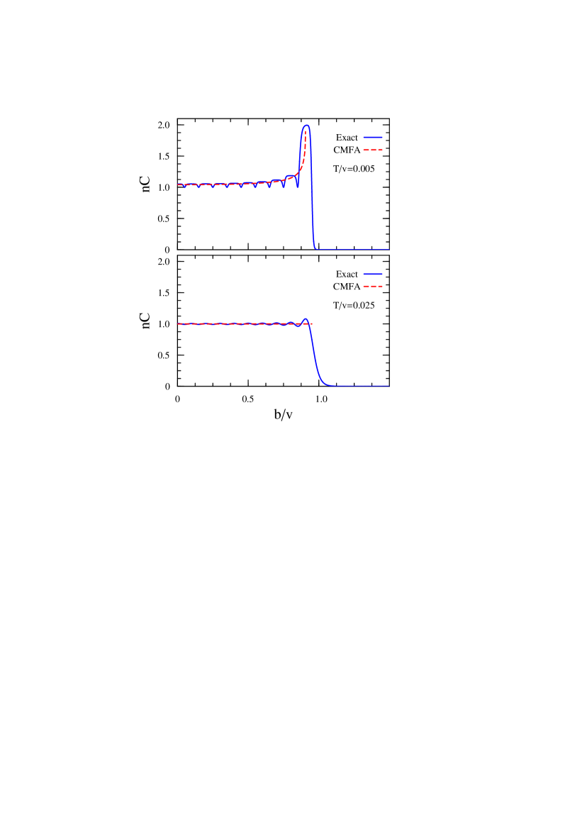
Figure 1: (Color online) Concurrence $C$ (multiplied by $n$) at low temperatures as a function of the magnetic field $b$ for $n=20$ spins coupled through the Hamiltonian (16) for $\gamma=1$. The curves depict exact and CMFA results for $T/v=0.005$ (top panel), where $C$ reaches its maximum value $2/n$ for $b\approx b_{c}$, and $T/v=1/2n=0.025$ (bottom panel), where the peak at $b\approx b_{c}$ is no longer prominent (Eq. (41)). The $T\rightarrow 0$ behavior for any $\gamma>0$ is identical except for the rescaling $v\rightarrow\gamma v$.

Thermal behavior. The concurrence (25) vanishes in symmetric states with fixed $S$ and $M$ if $S<n/2$, with the only exception of the case $|M|=S=n/2-1$, where $C=2/(n(n-1))$ (and $\alpha<0$). Hence, for $|b|<b_{c}$ we may expect a monotonous decrease of $C$ with increasing temperature, as the essential contribution will come from the states with $S=n/2$. The behavior for $|b|<b_{c}$ will be discussed in detail in the next subsection.

Nevertheless, for $T>0$ a weak pairwise entanglement also arises for $|b|>b_{c}$, i.e., when the ground state is fully separable, up to a limit temperature $T_{L}$ that becomes constant for large $b$. The behavior is thus similar to that arising with nearest neighbor $XX$ coupling CR.07 (and in agreement with the persistence of global entanglement for large fields in $XXZ$ models RC.05 ), although here $T_{L}$ will decrease as $n^{-1}$ for large $n$ with the scaling (19). To prove this result, we set $b>0$ and note that for $b-b_{c}\gg T$, we may just keep in $Z$ states with zero, one and two spins up ($M=-n/2+0,1,2$) for evaluating $C$ in the lowest non-zero order ($O(e^{-\beta b})$). This leads to

$$C \approx \frac{2e^{-\beta(b-b_{c})}}{n}[1-e^{-\beta v}-\sqrt{\frac{2n\eta}{n-1}}e^{-\beta\gamma v/n}]_{+}\,,$$ (27)

$$\eta = 1-(n-1)e^{-\beta v}+\mbox{$\frac{1}{2}$}n(n-3)e^{-2\beta v(1-1/n)}\,.$$ (28)

The field dependence in this limit is thus reduced to an exponential decay, with the limit temperature $b$-independent and determined by the root of the bracket in (27) (always positive for $T\rightarrow 0$ if $\gamma>0$). For large $n$, $C$ is positive just for low $T\propto n^{-1}$ and we may accurately neglect $e^{-\beta v}$ and set $\eta\approx 1$ in (27) (in which case it is just the result from the $S=n/2$ multiplet). This yields

$$T_{L}\approx\frac{2\gamma v}{n\ln[2n/(n-1)]}\approx\frac{2\gamma v}{n\ln 2+1}\,,\;\;b\gg b_{c}\,.$$ (29)

The maximum value reached by $C$ in this region (attained close to $T_{L}$) is very small ($\propto n^{-2}e^{-n(\ln 2)(b-\gamma v)/2}$).

III.3 CSPA and CMFA results for the $XX$ case

We start by describing the $XX$ case ($\gamma=1$ in (16)). In the representation (16b), the CSPA, Eq. (6), will lead to a two-dimensional integral over variables $(x,y)=r(\cos\phi,\sin\phi)$ associated with the linearized Hamiltonian $h(x,y)=bS_{z}-xS_{x}-yS_{y}+E_{0}/n$. Since $[H,S_{z}]=0$, both $Z(x,y)$ and $C_{\rm RPA}(x,y)$ will be independent of the orientation $\phi$, and the final expression can be written as

$$Z_{\rm CSPA}=\frac{n\beta}{2v}\!\!\int_{0}^{\infty}\!\!\!\!rdre^{-n\beta r^{2}/4v}Z(\lambda)C_{\rm RPA}(\lambda,\omega)\,,$$ (30)

where $\lambda=\sqrt{b^{2}+r^{2}}$ is the energy gap determined by $h(x,y)$ and

$$Z(\lambda)=e^{-\beta E_{0}}(2\cosh{\textstyle\frac{\beta\lambda}{2}})^{n}\,,$$ (31)

$$C_{\rm RPA}(\lambda,\omega)=\frac{\omega\sinh(\beta\lambda/2)}{\lambda\sinh(\beta\omega/2)}\,,$$ (32)

$$\omega=\sqrt{{\textstyle(\lambda-v\tanh\frac{\beta\lambda}{2})(\lambda-v\frac{b^{2}}{\lambda^{2}}\tanh\frac{\beta\lambda}{2})}}\,.$$ (33)

There is here a single collective RPA energy $\omega$. For temperatures lower than the mean field critical temperature $T_{c}$ (see below), Eq. (33) becomes imaginary for $r$ in an interval just below the stationary point (where $\omega=0$), leading to the CSPA breakdown when $\omega^{2}<-4\pi^{2}T^{2}$. This is first satisfied at $b=0$ and $r\approx v/2$, where $\omega\approx iv/2$, leading to a breakdown temperature $T^{*}\approx v/4\pi$ ($b=0$). $T^{*}$ decreases as $b$ increases, vanishing for $b>v$.

CMFA. The mean field equations (14) reduce here to

$$r=v\frac{r}{\lambda}\tanh{\frac{\beta\lambda}{2}},$$ (34)

and determine the minimum of the “Hartree” potential ${\cal F}(r)=nr^{2}/(4v)-T\ln Z(\lambda)$. We then need to distinguish between two regimes:

a) For $|b|<v$ and $T<T_{c}$, where

$$T_{c}=|b|/\ln\frac{1+|b|/v}{1-|b|/v}\,,\;\;(|b|<v)$$ (35)

the minimum of ${\cal F}(r)$ occurs at $r>0$. This solution of (34) breaks the rotational symmetry around the $z$ axes and is hence continuously degenerate ($\phi$ undetermined). In this case Eq. (34) implies that $\lambda$ is the root of $\lambda=v\tanh(\beta\lambda/2)$, being hence $b$-independent, the constraint $\lambda>|b|$ leading to the critical temperature (35) (which is a decreasing function of $|b|$, vanishing for $|b|\rightarrow v$ and approaching $v/2$ for $b\rightarrow 0$). The gaussian approximation (13) in the “intrinsic” variable $r$ leads then to

$$Z_{\rm CMFA} = e^{-\frac{n\beta}{4v}(\lambda^{2}-b^{2})}Z(\lambda){\textstyle\sinh\frac{\beta\lambda}{2}}\sqrt{\textstyle\frac{4\pi n}{\beta v(1-\chi)}}\,,$$ (36)

$$\chi = \mbox{$\frac{1}{2}$}\beta v/\cosh^{2}{\textstyle\frac{\beta\lambda}{2}}=\mbox{$\frac{1}{2}$}\beta v(1-{\textstyle\frac{\lambda^{2}}{v^{2}}})\,,$$ (37)

where the first two factors in (36) represent the MFA result and the rest the RPA and SPA corrections. Note that $\omega$ vanishes at this solution, in agreement with the broken continuous symmetry, but the RPA correction (32) remains finite (and essential) for $\omega\rightarrow 0$, with $C_{\rm RPA}(\lambda,\omega)\rightarrow\sinh(\beta\lambda/2)/(\beta\lambda/2)$.

It is apparent from (30) and (31) that in this region the approximation (36) will become increasingly accurate as $n$ increases (the $r$ fluctuation decreasing as $n^{-1}$), approaching the exact result for $n\rightarrow\infty$.

b) For $|b|>v$ or $T>T_{c}$, the minimum occurs at $r=0$ (normal solution of (34)). Direct application of Eq. (13) in the original variables $(x,y)$ leads then to

$$Z_{\rm CMFA} = Z(b)\frac{\sinh(\beta b/2)}{\sinh(\beta\omega/2)}\,,$$ (38)

where $\omega=b-v\tanh(\beta b/2)$.

Evaluation of the concurrence. Let us first examine the CMFA concurrence for $|b|<v$. Both $\langle S_{z}\rangle$ and $\langle S_{z}^{2}\rangle$ (Eq. (23)) will be determined just by the MFA contribution in (36), as the rest is $b$ independent, and given by

$$\langle S_{z}\rangle=-n\frac{b}{2v}\,,\;\;\langle S_{z}^{2}\rangle=\langle S_{z}\rangle^{2}+n\frac{T}{2v}\,,\;\;\;(T<T_{c})\,.$$ (39)

Hence, in this regime $\langle S_{z}\rangle$ is independent of $T$ (it is the value minimizing $b\langle S_{z}\rangle+v\langle S_{z}\rangle^{2}/n$) while the fluctuation $\langle S_{z}^{2}\rangle-\langle S_{z}\rangle^{2}$ increases linearly with $T$, reflecting a gaussian distribution $p(M)\propto e^{-\beta v(M-\langle S_{z}\rangle)^{2}/n}$. In contrast, $\langle S^{2}\rangle$ is affected by all terms in (36) and given by

$$\langle S^{2}\rangle=(\frac{n\lambda}{2v})^{2}+\frac{n}{2}[\frac{1-\chi[2-(1+\chi)T/v]}{(1-\chi)^{2}}]\,,$$ (40)

being $b$ independent. The first term is the Hartree part. For $T\rightarrow 0$, $\lambda/v\rightarrow 1$ while $\chi\rightarrow 0$, so that (40) approaches the right limit $\frac{n}{2}(\frac{n}{2}+1)$ owing to the RPA correction.

The CMFA concurrence is then obtained replacing Eqs. (39)-(40) in (25). As seen in Figs. (1)-(2), CMFA results turn out to be extremely accurate below the critical region, being undistinguishable from the exact ones if $T$ is not too small. For $T\rightarrow 0$, CMFA actually leads to the exact result but with $M$ replaced by the continuous variable $\mbox{$\frac{1}{2}$}nb/v$, representing then the exact $n\rightarrow\infty$ limit. Accordingly, it does not reproduce the stepwise behavior arising for $T\rightarrow 0$ and finite $n$, but remains close to the exact curve, correctly predicting the peak at $b\approx b_{c}$ (top panel in Fig. 1).

             

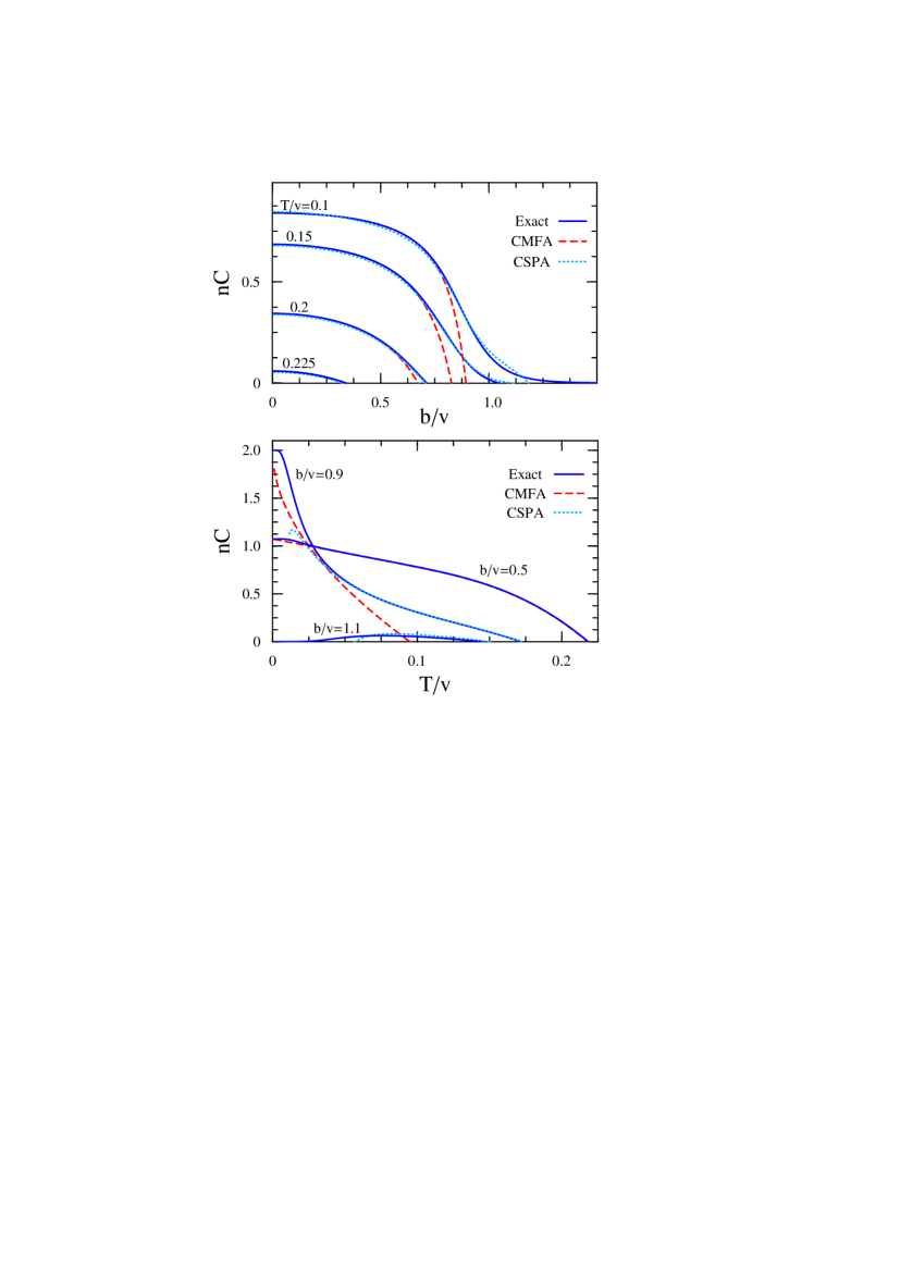
Figure 2: (Color online) Concurrence for $n=20$ spins and $\gamma=1$, as a function of the magnetic field at different temperatures (top) and as a function of temperature at different fields (bottom). Exact, CMFA and CSPA results are depicted, that of CMFA vanishing for $b/v=1.1$ (lower panel), where entanglement arises for $T>0$.

For low $T\ll T_{c}$, thermal effects in the CMFA will arise just from the $S_{z}$ fluctuation in (39), as we may still set $\chi=0$ in (40). As seen in the lower panel of Fig. 1, CMFA correctly predicts the low temperature

$$\tilde{T}=v/(2n)\,,$$ (41)

where the peak at $b\approx b_{c}$ disappears. In fact, at $T=\tilde{T}$ the CMFA concurrence has a strictly constant value $C=1/n$ for $b<b_{c}$, while for $T>\tilde{T}$ it starts to decrease with increasing field. We also note that for $T\leq\tilde{T}$ the CMFA result is applicable just for $b\leq b^{*}=b_{c}-v\sqrt{1-T/\tilde{T}}/n$, becoming complex for $b>b^{*}$ and being maximum just at $b=b^{*}$, where $C=(1+\sqrt{1-T/\tilde{T}})/n$. For $T>\tilde{T}$ it can however be applied right up to the limit field where $C$ vanishes in the CMFA.

As seen in Fig. 2, as $T$ increases beyond $\tilde{T}$, the CMFA provides practically exact results for $C$ even for $n=20$ if $|b|\lesssim\mbox{$\frac{1}{2}$}v$, since the concurrence in this region vanishes below $T_{c}$. However, the CMFA accuracy decreases significantly if $|b|$ is close to $v$. Moreover, for $|b|>v$ the CMFA (Eq. (38)) is not able to reproduce the exponentially small entanglement arising in this region. For large fields Eq. (38) leads to an expression similar to (27), i.e., $C\approx\frac{2}{n}e^{-\beta(b-v)}[\frac{n}{n-1}(1-e^{-\beta v})-\sqrt{\frac{2n\eta^{\prime}}{n-1}}]_{+}$, with $\eta^{\prime}\rightarrow 1$ for $T\ll v$, but the bracket is now always negative since it lacks the last exponential factor present in (27).

On the other hand, the full CSPA significantly improves CMFA results in the wide transitional region around $b\approx v$ arising for small $n$, as seen in Fig. 2. We may also appreciate the improvement over CMFA at field $b=0.9v$, where the CMFA result is inaccurate for all $T$ whereas the CSPA result is practically exact above the breakdown temperature, and also at $b=1.1v$, where the CMFA result vanishes while CSPA does predict the reentry of entanglement for $T>0$, albeit above a certain onset temperature. Nonetheless, the CSPA result cannot reproduce the exponentially small entanglement arising for very large fields either, since it vanishes above a certain limit field larger than $v$.

Results for large $n$. As $n$ increases, the width of the transitional region diminishes and the CMFA prediction for $|b|<v$ becomes increasingly accurate, being practically exact if $n\gtrsim 100$, as seen in Fig. 3. An expansion of the CMFA concurrence up to $O(n^{-1})$ leads to

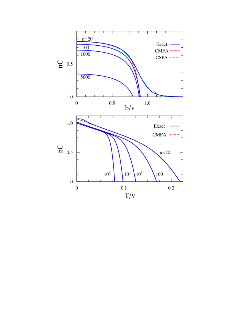
Figure 3: (Color online) Top: Concurrence as a function of the magnetic field at $T/v=0.1$ and different values of the number $n$ of spins, for $\gamma=1$. Exact, CMFA and CSPA results practically overlap for $n\gtrsim 100$, the concurrence vanishing for $n\gtrsim 8810$. Bottom: Concurrence as function of temperature at fixed field $b=0.5v$ and increasing values of $n$. Exact and CMFA results are undistinguishable for $n\gtrsim 100$.

$$C\approx\frac{1}{n}[\frac{1-\chi(2-(1+\chi)T/v)}{(1-\chi)^{2}}-\chi\frac{T}{v}(n+1)-\frac{2T/v}{1-b^{2}/v^{2}}]_{+}\,,$$ (42)

where the first term contains the RPA correction and provides the only positive contribution. For $T\ll T_{c}$, Eq. (34) leads to $\lambda/v\approx 1-2e^{-\beta\lambda}\approx 1-2e^{-\beta v}$, in which case $\chi\approx 2\beta ve^{-\beta v}$ and (42) reduces, up to order $\chi$, to

$$C\approx\frac{1}{n}[1-2ne^{-\beta v}-\frac{2T/v}{1-b^{2}/v^{2}}]_{+}\,.$$ (43)

Eq. (43) provides a simple yet accurate description of $C$ for $n\gtrsim 100$ if $|b|<v$. It implies an initial quadratic decrease with increasing field, and an initial $n$-independent linear decrease with increasing $T$ (Fig. 3) for $2ne^{-\beta v}\ll 1$, followed by a pronounced $n$-dependent decrease arising from the exponential term in (43) (which represents the effect from the $S=n/2-1$ multiplet). Note also that at fixed $T$, entanglement will disappear for $n\gtrsim\mbox{$\frac{1}{2}$}e^{\beta v}(1-2T/v)$ ($n\gtrsim 8810$ in top panel of Fig. 3).

Eq. (43) leads to a simple analytic expression for the limit field for entanglement $b_{L}(T)$,

$$b_{L}(T)\approx v\sqrt{1-\frac{2T/v}{1-2ne^{-\beta v}}}\,,$$ (44)

which is accurate for large $n$ and $T>T_{L}$ (Eq. (29)), as seen in Fig. 4. The inverse of (44) is the limit temperature $T_{L}(b)$, which is always lower than $T_{c}$ (Eq. (35)) and exhibits two regimes: For $T_{L}(b)\ll v$ ($2ne^{-v/T_{L}(b)}\ll 1$),

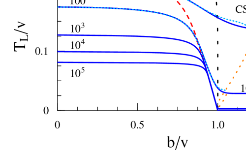
Figure 4: (Color online) Limit temperature for entanglement as a function of the magnetic field for different values of $n$ and $\gamma=1$. Exact, CMFA and CSPA (for $n=20$ and $n=100$) results are depicted, undistinguishable for $n\gtrsim 100$. $T_{L}$ decreases logarithmically with $n$ for $b<v$ and as $1/n$ for $b>v$. The sparse dashed line indicates the mean field critical temperature $T_{c}$.

$$T_{L}(b)\approx v-|b|\,,$$ (45)

which applies for large $n$ in a narrow field interval just before $|b|=v$, whereas for large $n$,

$$T_{L}(b)\approx\frac{v}{\ln 2n}[1-\frac{2}{(\ln 2n)^{2}(1-b^{2}/v^{2})}]\;\;\;\;(|b|<v)\,,$$ (46)

indicating a logarithmic decrease with $n$, in contrast with the $n^{-1}$ decrease arising for $|b|>v$ (Eq. (29)). For very large $n$, this yields $T_{L}(b)\approx v/\ln(2n)$, independent of $b$. We also note in Fig. 4 that for $n=20$ and 100, the CSPA improves the CMFA prediction of $T_{L}(b)$ in the critical region, up to the field region where $T_{L}(b)$ becomes close to the asymptotic value (29), although it also leads to a lower onset temperature (lower sparse dotted lines).

III.4 CSPA and CMFA in the $XXZ$ case

In the general case ($\gamma<1$) the CSPA leads to

$$Z_{\rm CSPA} = \frac{1}{4}\sqrt{\frac{n^{3}\beta^{3}}{\pi v^{3}(1-\gamma)}}\!\int_{0}^{\infty}\!\!\!\!\!\!rdr\!\!\int_{-\infty}^{\infty}\!\!\!\!\!\!\!\!dz\,e^{-\frac{n\beta}{4v}(r^{2}+\frac{z^{2}}{1-\gamma})}Z(\lambda)C_{\rm RPA}(\lambda,\omega)$$ (47)

where $Z(\lambda)$ and $C_{\rm RPA}(\lambda,\omega)$ are given by Eqs. (31)-(32) with $\lambda=\sqrt{(b-z)^{2}+r^{2}}$ and

$$\omega = \sqrt{{\textstyle(\lambda-v\tanh\frac{\beta\lambda}{2})(\lambda-v(1-\gamma\frac{r^{2}}{\lambda^{2}})\tanh\frac{\beta\lambda}{2})}}\,.$$ (48)

The mean field equations (14) become now

$$r=v\frac{r}{\lambda}\tanh\frac{\beta\lambda}{2}\,,\;\;\;z=(\gamma-1)v\frac{b-z}{\lambda}\tanh\frac{\beta\lambda}{2}\,.$$ (49)

In the symmetry-breaking phase ($r>0$), feasible for $\gamma>0$, the solution for $\lambda$ is then identical with that for $\gamma=1$, i.e., $\lambda=v\tanh(\beta\lambda/2)$, independent of $b$ and $\gamma$, in which case (49) leads to $b-z=b/\gamma$, independent of $T$ and $v$. This implies the rescaling $b\rightarrow b/\gamma$ at the CMFA level. This phase is then feasible for $|b|<\gamma v$ and $T<T_{c}$, where $T_{c}$ is given by Eq. (35) with $b\rightarrow b/\gamma$. The ensuing gaussian approximation to both $z$ and $r$ in (47) leads to the CMFA partition function

$$Z_{\rm CMFA}(\gamma,b,v,T)=Z_{\rm CMFA}(1,b/\gamma,v,T)/\sqrt{\gamma}\,,$$ (50)

where $Z_{\rm CMFA}(1,b,v,T)$ is the result (36).

From Eq. (50) we obtain $\langle S_{z}\rangle=-\mbox{$\frac{1}{2}$}nb/(\gamma v)$, and $\langle S_{z}^{2}\rangle-\langle S_{z}\rangle^{2}=\mbox{$\frac{1}{2}$}nT/(\gamma v)$ ($v\rightarrow\gamma v$ in (39 and hence in (41)), whereas $\langle S^{2}\rangle$ remains unchanged (Eq. (40)). The ensuing results for $C$ exhibit the same previous features, CMFA being accurate for $|b|<\gamma v$, and the CSPA improving the latter in the transitional region $|b|\approx\gamma v$. This can be seen in Fig. (5), whose upper panel depicts the quenching of the exact and approximate limit temperatures $T_{L}(b)$ for increasing $\gamma$.

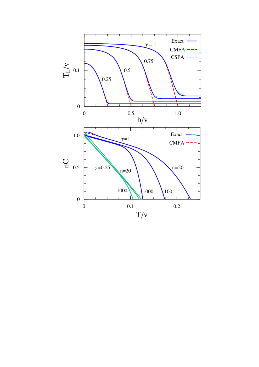
Figure 5: (Color online) Top: Limit temperature for entanglement as a function of the magnetic field $b$ for different values of the anisotropy $\gamma$ in (16) and $n=100$. Exact, CSPA and CMFA approximate results are depicted. Bottom: Concurrence $C$ as a function of temperature at zero field for $n=20$, $100$ and $1000$ and two different anisotropies.

For large $n$ and $T\ll T_{c}$, the CMFA leads now to

$$C\approx\frac{1}{n}[1-2ne^{-\beta v}-\frac{2T/(\gamma v)}{1-b^{2}/(\gamma v)^{2}}]_{+}\,,$$ (51)

which generalizes Eq. (43) and provides an accurate description for $n\gtrsim 100$ if $|b|<\gamma v$. For $\gamma<1$ it implies a more pronounced initial linear decrease with increasing $T$, as seen in the bottom panel of Fig. 5, which for low $\gamma$ may persist up to the vanishing of $C$ even for moderate sizes ($n\approx 100$ in Fig. 5). Eq. (51) leads to a limit field

$$b_{L}(T)\approx\gamma v\sqrt{1-\frac{2T/(\gamma v)}{1-2ne^{-\beta v}}}\,,$$ (52)

which describes the CMFA results of Fig. (5). It implies

$$T_{L}(b)\approx\gamma v[1-b^{2}/(\gamma v)^{2}]\,,\;\;\;\;\;$$

for $2ne^{-v/T_{L}(b)}\ll 1$, a condition which may now apply $\forall$ $|b|<\gamma v$ for moderate $n$ if $\gamma$ is sufficiently low, whereas for sufficiently large $n$,

$$T_{L}(b)\approx\frac{v}{\ln(2n)}[1-\frac{2/\gamma}{(\ln 2n)^{2}[1-b^{2}/(\gamma v)^{2}]}]\,,$$

decreasing logarithmically with $n$ and becoming independent of $\gamma$ and $b$ (for $|b|<\gamma v$) for very large $n$.

IV Conclusions

We have shown the feasibility of the CSPA approach for the determination of the pairwise entanglement in composite systems at finite temperature. The method is tractable, requiring just local diagonalizations and the evaluation of the generalized RPA energies, and unveils the crucial role played by the RPA correlations in the description of entanglement. It also leads to a consistent mean-field+RPA treatment (CMFA), which, as seen in the example considered, remains applicable and accurate in the presence of vanishing RPA energies, arising when continuous symmetries are broken at the mean field level.

In the $XXZ$ model considered, the CMFA provides an accurate analytic evaluation of the concurrence below the critical region ($|b|$ well below $b_{c}$) even in relatively small systems, providing exact results for large $n$ if $|b|<b_{c}$. The full CSPA allows to extend the accuracy to the critical region ($b\approx b_{c}$) in finite systems, above a low breakdown temperature, predicting a reentry of entanglement for $T>0$ for fields above but not too far from $b_{c}$, not detected at the CMFA level. Neither CMFA nor CSPA predict, however, the exponentially small entanglement arising for large fields at low non-zero temperatures.

The present results also reveal the rich thermal entanglement properties of the fully connected $XXZ$ model. We have shown by means of the CMFA that the limit temperature for pairwise entanglement decreases as $v/(\ln 2n)$ for very large $n$ if $|b|<b_{c}$, whereas for $|b|>b_{c}$ it decreases as $\gamma v/n$, becoming independent of $b$ for large fields. CMFA also shows that the $T=0$ peak in the concurrence just before the transition to the aligned state at $b=b_{c}$ disappears at a low temperature $\tilde{T}\approx\gamma v/(2n)$. The extension of the present approach to more complex systems, including spin chains with general anisotropic interactions, is currently under investigation.

The authors acknowledge support from CIC (RR) and CONICET (JMM and NC) of Argentina, respectively.

References

- (1) M.A. Nielsen and I. Chuang, Quantum Computation and Quantum Information, Cambridge Univ. Press (2000).
- (2) T.J. Osborne, M.A. Nielsen, Phys. Rev. A 66, 032110 (2002).
- (3) A. Osterloh et al, Nature (London) 416, 608 (2002).
- (4) G. Vidal, J.I. Latorre, E. Rico, A. Kitaev, Phys. Rev. Lett. 90, 227902 (2003).
- (5) T. Roscilde et al., Phys. Rev. Lett. 93, 167203 (2004).
- (6) C.H. Bennett et al., Phys. Rev. Lett. 70, 1895 (1993); Phys. Rev. Lett. 76, 722 (1996).
- (7) R.F. Werner, Phys. Rev. A 40, 4277 (1989).
- (8) M.C. Arnesen, S. Bose and V. Vedral, Phys. Rev. Lett. 87, 017901 (2001).
- (9) X. Wang, Phys. Rev. A 66, 044305 (2002); X. Wang, P. Zanardi, Phys. Lett. A 301, 1 (2002).
- (10) X. Wang, Phys. Rev. A 66, 034302 (2002); Phys. Rev. E 69, 066118 (2004).
- (11) M. Asoudeh, V. Karimipour, Phys. Rev. A 70, 052307 (2004); Phys. Rev. A 71 022308 (2005).
- (12) N. Canosa, R. Rossignoli, Phys. Rev. A 69, 052306 (2004).
- (13) A.C. Doherty, P.A. Parrilo, and F.M. Spedalieri, Phys. Rev. A 69, 022308 (2004).
- (14) R. Rossignoli, N. Canosa, Phys. Rev. A 72, 012335 (2005); N. Canosa, R. Rossignoli, Phys. Rev. A 73, 022347 (2006).
- (15) B. Mühlschlegel, D.J. Scalapino, and R. Denton, Phys. Rev. B 6, 1767 (1972).
- (16) G. Puddu, P.F. Bortignon, and R.A. Broglia, Ann. Phys. (N.Y.) 206, 409 (1991).
- (17) H. Attias and Y. Alhassid, Nucl. Phys. A 625, 565 (1997).
- (18) R. Rossignoli, N. Canosa, Phys. Lett. B 394, 242 (1997).
- (19) R. Rossignoli, N. Canosa, and P. Ring, Phys. Rev. Lett. 80, 1853 (1998); Ann. Phys. (N.Y.) 275, 1 (1999).
- (20) R.L. Stratonovich, Dokl. Akad. Nauk. SSSR 115 1097 (1957) (trans. Soviet Phys. Dokl. 2 458 (1958)); J. Hubbard, Phys. Rev. Lett. 3 77 (1959).
- (21) K. Kaneko and M. Hasegawa, Phys. Rev. C 72, 061306(R) (2005); Phys. Rev. C 72, 024307 (2005).
- (22) R. Rossignoli and N. Canosa, Phys. Rev. B 63, 134523 (2001); N. Canosa and R. Rossignoli, Phys. Rev. B 62, 5886 (2000).
- (23) D.P. DiVincenzo et al, Nature (London) 408, 339 (2000).
- (24) D. Loss, and D.P. DiVincenzo, Phys. Rev. A 57, 120 (1998); G. Burkard, D. Loss, and D.P. DiVincenzo, Phys. Rev. B 59, 2070 (1999).
- (25) S.C. Benjamin, S. Bose, Phys. Rev. Lett. 90, 247901 (2003); Phys. Rev. A 70, 032314 (2004).
- (26) A. Imamoglu et al, Phys. Rev. Lett. 83, 4204 (1999).
- (27) Y. Makhlin, G. Schön and A. Shnirman, Rev. Mod. Phys. 73, 357 (2001).
- (28) J. Vidal, G. Palacios, and R. Mosseri, Phys. Rev. A 69, 022107 (2004).
- (29) S. Dusuel and J. Vidal, Phys. Rev. Lett. 93, 237204 (2004).
- (30) J. Vidal, Phys. Rev. A 73, 062318 (2006).
- (31) S. Hill and W.K. Wootters, Phys. Rev. Lett. 78, 5022 (1997); W.K. Wootters, Phys. Rev. Lett. 80, 2245 (1998).
- (32) P. Rungta and C.M. Caves, Phys. Rev. A 67, 012307 (2003).
- (33) C.H. Bennett, D.P. DiVincenzo, J.A. Smolin, W.K. Wootters, Phys. Rev. A 54, 3824 (1996).
- (34) A. Peres, Phys. Rev. Lett. 77, 1413 (1996).
- (35) M. Koashi, V. Buz̃ek, and N. Imoto, Phys. Rev. A 62, 050302(R) (2000); W. Dür, Phys. Rev. A 63, 020303 (2001).
- (36) N. Canosa, R. Rossignoli, Phys. Rev. A 75 032350 (2007).