Coherent States of Accelerated Relativistic Quantum Particles, Vacuum Radiation and the Spontaneous Breakdown of the Conformal SU(2,2) Symmetry

M. Calixto^1,2, E. Pérez-Romero¹ and V. Aldaya²

Abstract

• We give a quantum mechanical description of accelerated relativistic particles in the framework of Coherent States (CS) of the (3+1)-dimensional conformal group $SU(2,2)$, with the role of accelerations played by special conformal transformations and with the role of (proper) time translations played by dilations. The accelerated ground state $\tilde{\varphi}_{0}$ of first quantization is a CS of the conformal group. We compute the distribution function giving the occupation number of each energy level in $\tilde{\varphi}_{0}$ and, with it, the partition function ${\cal Z}$, mean energy ${\cal E}$ and entropy ${\cal S}$, which resemble that of an “Einstein Solid”. An effective temperature ${\cal T}$ can be assigned to this “accelerated ensemble” through the thermodynamic expression $d{\cal E}/d{\cal S}$, which leads to a (non linear) relation between acceleration and temperature different from Unruh’s (linear) formula. Then we construct the corresponding conformal-$SU(2,2)$-invariant second quantized theory and its spontaneous breakdown when selecting Poincaré-invariant degenerated $\theta$-vacua (namely, coherent states of conformal zero modes). Special conformal transformations (accelerations) destabilize the Poincaré vacuum and make it to radiate.

PACS: 02.20.Qs, 03.65.Fd, 03.65.Pm, 11.30.Qc, 67.40.Db,

MSC: 81R30, 81R05, 42B05, 30H20, 42C15

Keywords: coherent states; accelerated frames; Lie-group representation theory; conformal relativity; conformal invariant quantum mechanics; spontaneous symmetry breaking; zero modes; vacuum radiation; ground state excitations; Fulling-Davies-Unruh effect.

1 Introduction

The quantum analysis of accelerated frames of reference has been studied mainly in connection with Quantum Field Theory (QFT) in curved space-time. For example, the case of the quantization of a Klein-Gordon field in Rindler coordinates (see e.g. [1, 2] and Appendix A for a short review) entails a global mutilation of flat space-time, with the appearance of event horizons, and leads to a quantization inequivalent to the standard Minkowski quantization. Physically one says that, whereas the Poincaré-invariant (Minkowskian) vacuum $|0\rangle$ in QFT looks the same to any inertial observer (i.e., it is stable under Poincaré transformations), it converts into a thermal bath of radiation with temperature

$$T=\frac{\hbar a}{2\pi vk_{B}}$$ (1)

in passing to a uniformly accelerated frame ($a$ denotes the acceleration, $v$ the speed of light and $k_{B}$ the Boltzmann constant). This is called the Fulling-Davies-Unruh effect [1, 3, 4], which shares some features with the (black-hole) Hawking [5] effect. Its explanation relies heavily upon Bogoliubov transformations, which find a natural explanation in the framework of Coherent States (CS) and squeezed states [6].

In this article we also approach the quantum analysis of accelerated frames from a CS perspective but the scheme is rather different, although it shares some features with the standard approach commented before. The situation will be similar in some respects to quantum many-body condensed mater systems describing, for example, superfluidity and superconductivity, where the ground state mimics the quantum vacuum in many respects and quasi-particles (particle-like excitations above the ground state) play the role of matter. We shall enlarge the Poincaré symmetry ${\cal P}$ to account for uniform accelerations and then we shall spontaneously break it down back to Poincaré by selecting appropriate “non-empty vacua” stable under ${\cal P}$. Then the action of broken symmetry transformations (accelerations) will destabilize/excitate the vacuum and make it to radiate. The candidate for an enlargement of ${\cal P}$ will be the conformal group in (3+1)-dimensions $SO(4,2)$ incorporating dilations and special conformal transformations (STC)

$$x^{\mu}\rightarrow{x^{\prime}}^{\mu}=\frac{x^{\mu}+c^{\mu}x^{2}}{1+2cx+c^{2}x^{2}},$$ (2)

which can be interpreted as transitions to systems of relativistic, uniformly accelerated observers with acceleration $a=2c$ (see e.g. Ref. [7, 8, 9] and later on Eq. (9)). From the conformal symmetry point of view, Poincaré-invariant vacua are regarded as a coherent states of conformal zero modes, which are undetectable (“dark”) by inertial observers but unstable under special conformal transformations.

A previous preliminary attempt to analyze quantum accelerated frames from a conformal group perspective was made in the reference [10] (see also [11]), where a quite involved “second quantization formalism on a group $G$” was developed and applied to the (finite part of the) conformal group in (1+1) dimensions, $SO(2,2)\simeq SO(2,1)\times SO(2,1)$, which consists of two copies of the pseudo-orthogonal group $SO(2,1)$ (left- and right-moving modes, respectively). Here we shall use more conventional methods of quantization and we shall work in realistic (3+1) dimensions, using the (more involved) conformal group $SO(4,2)\simeq SU(2,2)/\mathbb{Z}_{4}$. New consequences of this group-theoretical approach are obtained here, regarding a similitude between the accelerated ground state and the “Einstein Solid”, the computation of entropies and a deviation from the Unruh’s formula (1).

We would like to mention that (near-horizon two-dimensional) conformal symmetry has also played a fundamental role in the microscopic description of the Hawking effect. In fact, there is strong evidence that conformal field theories provide a universal (independent of the details of the particular quantum gravity model) description of low-energy black hole entropy, which is only fixed by symmetry arguments (see e.g. [12, 13]). Here, the Virasoro algebra turns out to be the relevant subalgebra of surface deformations of the horizon of an arbitrary black hole and constitutes the general gauge (diffeomorphism) principle that governs the density of states. However, in 3+1 dimensions, conformal invariance is necessarily global (finite-(15)-dimensional). In this paper we shall study zero-order effects that gravity has on quantum theory (uniform accelerations). To account for higher-order effects (like non-constant accelerations) in a group-theoretical framework, we should firstly promote the 3+1 conformal symmetry SO(4,2) to a higher-(infinite)-dimensional symmetry. This is not a trivial task, although some steps have been done by the authors in this direction (see e.g. [14, 15, 11, 16, 17]).

The organization of the paper is as follows. In Section 2 we discuss the group theoretical backdrop (conformal transformations, infinitesimal generators and commutation relations) and justify the interpretation of special conformal transformations as transitions to relativistic uniform accelerated frames of reference. In Section 3 we construct the Hilbert space and an orthonormal basis for our conformal particle in 3+1 dimensions, based on an holomorphic square-integrable irreducible representation of the conformal group on the eight-dimensional phase space $\mathbb{D}_{4}=SO(4,2)/SO(4)\times SO(2)$ inside the complex Minkowski space $\mathbb{C}^{4}$. In Section 4 we remind the general definition of CS of a group $G$, highlight the Poincaré invariance of the ground state, construct the accelerated ground state as a CS of the conformal group and calculate the distribution function, mean energy, partition function and entropy of this accelerated ground state, seen as a statistical ensemble. This leads us to interpret the accelerated ground state as an Einstein Solid, to obtain a deviation from the Unruh’s formula (1) and to discuss on the existence of a maximal acceleration. In Section 5 we deal with the second-quantized (many-body) theory, where Poincaré-invariant (degenerated) pseudo-vacua are coherent states of conformal zero modes. Selecting one of this Poincaré-invariant pseudo-vacua spontaneously breaks the conformal invariance and leads to vacuum radiation. Section 6 is left for conclusions and outlook. In addition, two appendices are also included. Appendix A reminds Rindler coordinates and Bogoliubov transformations in the standard derivation of Unruh effect and Appendix B reports on the underlying gauge-invariant Lagrangian formalism behind our quantum model of conformal particles.

2 The Conformal Group and its Generators

The conformal group in 3+1 dimensions, $SO(4,2)$, is composed by Poincaré ${\cal P}=SO(3,1)\circledS\mathbb{R}^{4}$ [semidirect product of spacetime translations $b^{\mu}\in\mathbb{R}^{4}$ times Lorentz $\Lambda^{\mu}_{\nu}\in SO(3,1)$] transformations augmented by dilations ($e^{\tau}\in\mathbb{R}_{+}$) and relativistic uniform accelerations (special conformal transformations, $c^{\mu}\in\mathbb{R}^{4}$) which, in Minkowski spacetime, have the following realization:

$$\begin{array}[]{rcl}x^{\prime\mu}&=&x^{\mu}+b^{\mu},\;\;x^{\prime\mu}=\Lambda^{\mu}_{\nu}(\omega)x^{\nu},\\ x^{\prime\mu}&=&e^{\tau}x^{\mu},\;\;x^{\prime\mu}=\frac{x^{\mu}+c^{\mu}x^{2}}{1+2cx+c^{2}x^{2}},\end{array}$$ (3)

respectively. The infinitesimal generators (vector fields) of the transformations (3) are easily deduced:

$$\begin{array}[]{rcl}P_{\mu}&=&\frac{\partial}{\partial x^{\mu}},\;\;M_{\mu\nu}=x_{\mu}\frac{\partial}{\partial x^{\nu}}-x_{\nu}\frac{\partial}{\partial x^{\mu}},\\ D&=&x^{\mu}\frac{\partial}{\partial x^{\mu}},\;\;K_{\mu}=-2x_{\mu}x^{\nu}\frac{\partial}{\partial x^{\nu}}+x^{2}\frac{\partial}{\partial x^{\mu}}\end{array}$$ (4)

and they close into the conformal Lie algebra

$$\begin{array}[]{rcl}\left[M_{\mu\nu},M_{\rho\sigma}\right]&=&\eta_{\nu\rho}M_{\mu\sigma}+\eta_{\mu\sigma}M_{\nu\rho}-\eta_{\mu\rho}M_{\nu\sigma}-\eta_{\nu\sigma}M_{\mu\rho},\\ \left[P_{\mu},M_{\rho\sigma}\right]&=&\eta_{\mu\rho}P_{\sigma}-\eta_{\mu\sigma}P_{\rho},\;\;\left[P_{\mu},P_{\nu}\right]=0,\\ \left[K_{\mu},M_{\rho\sigma}\right]&=&\eta_{\mu\rho}K_{\sigma}-\eta_{\mu\sigma}K_{\rho},\;\;\left[K_{\mu},K_{\nu}\right]=0,\\ \left[D,P_{\mu}\right]&=&-P_{\mu},\;\;\left[D,K_{\mu}\right]=K_{\mu},\;\;\left[D,M_{\mu\nu}\right]=0,\\ \left[K_{\mu},P_{\nu}\right]&=&2(\eta_{\mu\nu}D+M_{\mu\nu}).\end{array}$$ (5)

The conformal quadratic Casimir operator

$$C_{2}=D^{2}-\frac{1}{2}M_{\mu\nu}M^{\mu\nu}+\frac{1}{2}(P_{\mu}K^{\mu}+K_{\mu}P^{\mu}),$$ (6)

generalizes the Poincaré Casimir $P^{2}=P_{\mu}P^{\mu}$ which, for scalar fields $\phi$, leads to the Klein-Gordon equation $P^{2}\phi=m^{2}_{0}\phi$, with $m^{2}_{0}$ the squared rest mass. The fact that $[D,P^{2}]=-2P^{2}$ implies that conformal fields must be either massless or to have a continuous mass spectrum (see e.g. the classical Refs. [18] and [19]). Actually, just like the Poincaré invariant mass $m_{0}$ comprises a continuum of “Galilean” masses $m$, a conformally invariant mass $m_{00}$ can be defined by the Casimir (6), which comprises a continuum of Poincaré masses $m_{0}$. The eigenvalue equation $C_{2}\phi=m_{00}^{2}\phi$ can be seen as a generalized Klein-Gordon equation, where $D$ replaces $P_{0}$ as the (proper) time evolution generator and $m_{00}$ replaces $m_{0}$ (see Appendix B for more information and [18] for the formulation of other conformally-invariant massive field equations of motion in generalized Minkowski space).

In this article we shall deal with discrete series representations of the conformal group having continuous mass spectrum and the corresponding wavefunctions having support on the whole four-dimensional Minkowski space-time, with the dilation parameter $\tau$ playing the role of a proper time. We shall report on this model of conformal quantum particles later on Sec. 3. The reader can also consult our recent reference [20] for a gauge-invariant Lagrangian approach (of nonlinear sigma-model type), using a generalized Dirac method for the quantization of constrained systems. We give here a flavor of this approach in the Appendix B.

2.1 Special conformal transformations as transitions to uniform relativistic accelerated frames

The interpretation of special conformal transformations (2) as transitions from inertial reference frames to systems of relativistic, uniformly accelerated observers was identified many years ago by [7, 8, 9]. More precisely, denoting by $u^{\mu}=\frac{dx^{\mu}}{d\tau}$ and $a^{\mu}=\frac{du^{\mu}}{d\tau}$ the four-velocity and four-acceleration of a point particle, respectively, the relativistic motion with constant acceleration is characterized by the usual condition [21]:

$$a_{\mu}a^{\mu}=-{\rm g}^{2},$$ (7)

where ${\rm g}$ is the magnitude of the acceleration in the instantaneous rest system. From $u_{\mu}u^{\mu}=1$ (in $v=1$ unities) and (7), we can derive the differential equation to be satisfied for all systems with constant relative acceleration:

$$\frac{da^{\mu}}{d\tau}={\rm g}^{2}u^{\mu}.$$ (8)

Hill [7] (see also [8] and [9]) proved that the kinematical invariance group of (8) is precisely the conformal group $SO(4,2)$. Here we shall provide a simple explanation of this fact. For simplicity, let us take an acceleration along the “z” axis: $c^{\mu}=(0,0,0,c)$, and the temporal path $x^{\mu}=(t,0,0,0)$. Then the transformation (2) reads:

$$t^{\prime}=\frac{t}{1-c^{2}t^{2}}\;,\;\;\;\;\;\;z^{\prime}=\frac{ct^{2}}{1-c^{2}t^{2}}.$$ (9)

Writing $z^{\prime}$ in terms of $t^{\prime}$ gives the usual formula for the relativistic uniform accelerated (hyperbolic) motion:

$$z^{\prime}=\frac{1}{a}(\sqrt{1+{a^{2}t^{\prime 2}}}-1)$$ (10)

with $a=2c$.

Let us say that at least two alternative meanings of special conformal transformations (STC) have also been proposed [22, 23]. One is related to the Weyl’s idea of different lengths in different points of space time [22]: “the rule for measuring distances changes at different positions”. Other is Kastrup’s interpretation of SCT as geometrical gauge transformations of the Minkowski space [23].

3 A Model of Conformal Quantum Particles

In this Section we report on a model for quantum particles with conformal symmetry. The reader can find more details in the Reference [20], where we formulate a gauge invariant nonlinear sigma-model on the conformal group and quantize it according to a generalized Dirac method for constrained systems.

3.1 The compactified Minkowski space and the isomorphism $SO(4,2)=SU(2,2)/\mathbb{Z}_{4}$

In [20] (see also the Appendix B) it is shown how the Minkowski space arises as the support of constrained wave functions on the conformal group. Actually, the compactified Minkowski space $\mathbb{M}_{4}=\mathbb{S}^{3}\times_{\mathbb{Z}_{2}}\mathbb{S}^{1}$ naturally lives inside the conformal group $SO(4,2)$ as the coset $\mathbb{M}_{4}=SO(4,2)/{\cal W}$, where ${\cal W}$ denotes the Weyl subgroup generated by $K_{\mu},M_{\mu\nu}$ and $D$ (i.e., a Poincaré subgroup ${\cal P}$ augmented by the dilations $\mathbb{R}^{+}$). The Weyl group ${\cal W}$ is the stability subgroup (the little group in physical usage) of $x^{\mu}=0$. The conformal group acts transitively on $\mathbb{M}_{4}$ and free from singularities.

Instead of $SO(4,2)$, we shall work by convenience with its four covering group:

$$SU(2,2)=\left\{g=\left(\begin{array}[]{cc}A&B\\ C&D\end{array}\right)\in{\rm Mat}_{4\times 4}(\mathbb{C}):g^{\dagger}\Gamma g=\Gamma,\det(g)=1\right\},$$ (11)

where $\Gamma$ denotes a hermitian form of signature $(++--)$.

The conformal Lie algebra (5) can also be realized in terms of gamma matrices in, for instance, the Weyl basis

$$\gamma^{\mu}=\left(\begin{array}[]{cc}0&\sigma^{\mu}\\ \check{\sigma}^{\mu}&0\end{array}\right),\;\;\gamma^{5}=i\gamma^{0}\gamma^{1}\gamma^{2}\gamma^{3}=\left(\begin{array}[]{cc}-\sigma^{0}&0\\ 0&\sigma^{0}\end{array}\right),$$ (12)

where $\check{\sigma}^{\mu}\equiv\sigma_{\mu}$ (we are using the convention $\eta={\rm diag}(1,-1,-1,-1)$) and $\sigma^{\mu}$ are the standard Pauli matrices

$$\sigma^{0}=I=\left(\begin{array}[]{cc}1&0\\ 0&1\end{array}\right),\;\sigma^{1}=\left(\begin{array}[]{cc}0&1\\ 1&0\end{array}\right),\;\sigma^{2}=\left(\begin{array}[]{cc}0&-i\\ i&0\end{array}\right),\;\sigma^{3}=\left(\begin{array}[]{cc}1&0\\ 0&-1\end{array}\right).$$ (13)

Indeed, the choice

$$D = \frac{\gamma^{5}}{2},\;M^{\mu\nu}=\frac{\left[\gamma^{\mu},\gamma^{\nu}\right]}{4}=\frac{1}{4}\left(\begin{array}[]{cc}\sigma^{\mu}\check{\sigma}^{\nu}-\sigma^{\nu}\check{\sigma}^{\mu}&0\\ 0&\check{\sigma}^{\mu}\sigma^{\nu}-\check{\sigma}^{\nu}\sigma^{\mu}\end{array}\right),$$ (16)

$$P^{\mu} = \gamma^{\mu}\frac{1+\gamma^{5}}{2}=\left(\begin{array}[]{cc}0&\sigma^{\mu}\\ 0&0\end{array}\right),\;K^{\mu}=\gamma^{\mu}\frac{1-\gamma^{5}}{2}=\left(\begin{array}[]{cc}0&0\\ \check{\sigma}^{\mu}&0\end{array}\right)$$ (21)

fulfills the commutation relations (5). These are the Lie algebra generators of the fundamental representation of $SU(2,2)$.

The group $SU(2,2)$ acts transitively on the compactified Minkowski space $\mathbb{M}_{4}$, which can be identified with the set of hermitian $2\times 2$ matrices $X=x_{\mu}\sigma^{\mu}$, as follows:

$$X\to X^{\prime}=(AX+B)(CX+D)^{-1}.$$ (22)

With this identification, the transformations (3) can be recovered from (22) as follows:

• Standard Lorentz transformations, $x^{\prime\mu}=\Lambda^{\mu}_{\nu}(\omega)x^{\nu}$, correspond to $B=C=0$ and $A=D^{-1{\dagger}}\in SL(2,\mathbb{C})$, where we are making use of the homomorphism (spinor map) between $SO^{+}(3,1)$ and $SL(2,\mathbb{C})$ and writing $X^{\prime}=AXA^{\dagger},A\in SL(2,\mathbb{C})$ instead of $x^{\prime\mu}=\Lambda^{\mu}_{\nu}x^{\nu}$.

• Dilations correspond to $B=C=0$ and $A=D^{-1}=e^{\tau/2}I$

• Spacetime translations are $A=D=I$, $C=0$ and $B=b_{\mu}\sigma^{\mu}$.

• Special conformal transformations correspond to $A=D=I$ and $C=c_{\mu}\sigma^{\mu},B=0$ by noting that $\det(CX+I)=1+2cx+c^{2}x^{2}$:

  $$X^{\prime}=X(CX+I)^{-1}\leftrightarrow x^{\prime\mu}=\frac{x^{\mu}+c^{\mu}x^{2}}{1+2cx+c^{2}x^{2}}$$

3.2 Unirreps of the conformal group: discrete series

We shall consider the complex extension of the compactified Minkowski space $\mathbb{M}_{4}=U(2)$ to the 8-dimensional conformal (phase) space:

$$\mathbb{D}_{4}=U(2,2)/U(2)^{2}=\{Z\in{\rm Mat}_{2\times 2}(\mathbb{C}):I-ZZ^{\dagger}>0\},$$ (23)

of which $\mathbb{M}_{4}=\{Z\in{\rm Mat}_{2\times 2}(\mathbb{C}):I-ZZ^{\dagger}=0\}$ is the Shilov boundary. It can be proved (see e.g. [20] and [24]) that the following action

$$[U_{\lambda}(g)\phi](Z)=|CZ+D|^{-\lambda}\phi(Z^{\prime}),\;Z^{\prime}=(AZ+B)(CZ+D)^{-1}$$ (24)

constitutes a unitary irreducible representation of $SU(2,2)$ on the Hilbert space ${\cal H}_{\lambda}(\mathbb{D}_{4})$ of square-integrable holomorphic functions $\phi$ with invariant integration measure

$$d\mu_{\lambda}(Z,Z^{\dagger})=\pi^{-4}(\lambda-1)(\lambda-2)^{2}(\lambda-3)\det(I-ZZ^{\dagger})^{\lambda-4}|dZ|,$$

where the label $\lambda\in\mathbb{Z},\lambda\geq 4$ is the conformal, scale or mass dimension ($|dZ|$ denotes the Lebesgue measure in $\mathbb{C}^{4}$). The factor $\pi^{-4}(\lambda-1)(\lambda-2)^{2}(\lambda-3)$ in $d\mu_{\lambda}(Z,Z^{\dagger})$ is chosen so that the constant function $\phi(Z)=1$ has unit norm. Besides the conformal dimension $\lambda$, the discrete series representations of $SU(2,2)$ have two extra spin labels $s_{1},s_{2}\in\mathbb{N}/2$ associated with the (stability) subgroup $SU(2)\times SU(2)$. Here we shall restrict ourselves to scalar fields ($s_{1}=s_{2}=0$) for the sake of simplicity (see e.g. [20] for the spinning unirreps of $SU(2,2)$). The reduction of this representation into unitary irreducible representations of the Poincaré subgroup indicates that we are dealing with fields with a continuous mass spectrum extending from zero to infinity [25].

3.3 The Hilbert space of our conformal particle

It has been proved in [24] that the infinite set of homogeneous polynomials

$$\varphi_{q_{1},q_{2}}^{j,m}(Z)=\sqrt{\frac{2j+1}{\lambda-1}\binom{m+\lambda-2}{\lambda-2}\binom{m+2j+\lambda-1}{\lambda-2}}\det(Z)^{m}{\cal D}^{j}_{q_{1},q_{2}}(Z),$$ (25)

with

$${\cal D}^{j}_{q_{1},q_{2}}(Z)=\sqrt{\frac{(j+q_{1})!(j-q_{1})!}{(j+q_{2})!(j-q_{2})!}}\sum_{p=\max(0,q_{1}+q_{2})}^{\min(j+q_{1},j+q_{2})}\tbinom{j+q_{2}}{p}\tbinom{j-q_{2}}{p-q_{1}-q_{2}}z_{11}^{p}z_{12}^{j+q_{1}-p}z_{21}^{j+q_{2}-p}z_{22}^{p-q_{1}-q_{2}}$$ (26)

the standard Wigner’s ${\cal D}$-matrices ($j\in{\mathbb{N}}/2$), verifies the following closure relation (the reproducing Bergman kernel or $\lambda$-extended MacMahon-Schwinger’s master formula):

$$\sum_{j\in{\mathbb{N}}/2}\sum^{\infty}_{m=0}\sum^{j}_{q_{1},q_{2}=-j}\overline{\varphi_{q_{1},q_{2}}^{j,m}({Z})}\varphi_{q_{1},q_{2}}^{j,m}(Z^{\prime})=\frac{1}{\det(I-Z^{\dagger}Z^{\prime})^{\lambda}}$$ (27)

and constitutes an orthonormal basis of ${\cal H}_{\lambda}(\mathbb{D}_{4})$ (the sum on $j$ accounts for all non-negative half-integer numbers). The identity (27) will be usefull for us in the sequel.

3.4 Hamiltonian and energy spectrum

In [20] we have argued that the dilation operator $D$ plays the role of the Hamiltonian of our conformal quantum theory. Actually, the replacement of time translations by dilations as kinematical equations of motion has already been considered in the literature (see e.g. [26] and in [27]), when quantizing field theories on space-like Lorentz-invariant hypersurfaces $x^{2}=x^{\mu}x_{\mu}=\tau^{2}=$constant. In other words, if one wishes to proceed from one surface at $x^{2}=\tau_{1}^{2}$ to another at $x^{2}=\tau_{2}^{2}$, this is done by scale transformations; that is, $D=\frac{\partial}{\partial\tau}$ is the evolution operator in a proper time $\tau$. We must say that other possibilities exist for choosing a conformal Hamiltonian, namely the combination $\tilde{P}_{0}=(P_{0}+K_{0})/2$, which has been used in [19].

From the general expression (24), we can compute the finite left-action of dilations ($B=0=C$ and $A=e^{\tau/2}\sigma^{0}=D^{-1}\Rightarrow g=e^{\tau/2}{\rm diag}(1,1,-1,-1)$) on wave functions,

$$[U_{\lambda}(g)\phi](Z)=e^{\lambda\tau}\phi(e^{\tau}Z).$$ (28)

The infinitesimal generator of this transformation is the Hamiltonian operator:

$$H=\lambda+\sum_{i,j=1}^{2}Z_{ij}\frac{\partial}{\partial Z_{ij}}=\lambda+z_{\mu}\frac{\partial}{\partial{z_{\mu}}},$$ (29)

where we have set $Z=z_{\mu}\sigma^{\mu}$ in the last equality. This Hamiltonian has the form of that of a four-dimensional (relativistic) harmonic oscillator in the Bargmann representation. The set of functions (25) constitutes a basis of Hamiltonian eigenfunctions (homogeneous polynomials) with energy eigenvalues ${E}_{n}^{\lambda}$ (the homogeneity degree) given by:

$$H\varphi_{q_{1},q_{2}}^{j,m}={E}_{n}^{\lambda}\varphi_{q_{1},q_{2}}^{j,m},\;\;{E}_{n}^{\lambda}=\lambda+n,\;\;n=2j+2m.$$ (30)

Actually, each energy level ${E}_{n}^{\lambda}$ is $(n+1)(n+2)(n+3)/6$ times degenerated (just like a four-dimensional harmonic oscillator). This degeneracy coincides with the number of linearly independent polynomials $\prod_{i,j=1}^{2}Z_{ij}^{n_{ij}}$ of fixed degree of homogeneity $n=\sum_{i,j=1}^{2}n_{ij}$. This also proves that the set of polynomials (25) is a basis for analytic functions $\phi\in{\cal H}_{\lambda}(\mathbb{D}_{4})$. The spectrum is equi-spaced and bounded from below, with ground state $\varphi_{0,0}^{0,0}=1$ and zero-point energy $E_{0}^{\lambda}=\lambda$ (the conformal, scale or mass dimension).

4 Coherent States of Accelerated Relativistic Particles, Distribution Functions and Mean Values

Before introducing coherent states of $G=SU(2,2)$, let us briefly remind some general definitions and constructions for a general group $G$. More information on coherent states can be found in standard text books like [28, 29, 30].

4.1 A brief on coherent states

Essential ingredients to define and construct Coherent States (CS) on a given symmetry (Lie) group $G$ are the following. Firstly, we need a unitary representation $U$ of $G$ on a Hilbert space $({\cal H},\langle\cdot|\cdot\rangle)$. Consider also the space $L^{2}(G,dg)$ of square-integrable complex functions $\Psi$ on $G$, where $dg=d(g^{\prime}g),\,\forall g^{\prime}\in G$, stands for the left-invariant Haar measure on $G$. A non-zero vector $\varphi^{0}\in{\cal H}$ is called admissible (or a fiducial vector) if $\Phi(g)\equiv\langle U(g)\varphi^{0}|\varphi^{0}\rangle\in L^{2}(G,dg)$. A unitary representation $U$ for which admissible vector exists is called square integrable. Assuming that the representation $U$ is irreducible, and that there exists a function $\varphi_{0}$ admissible, then a system of CS of ${\cal H}$ associated to (or indexed by) $G$ is defined as the set of functions in the orbit of $\varphi^{0}$ under $G$:

$$\varphi_{g}^{0}\equiv U(g)\varphi^{0},\;\;g\in G,$$ (31)

and they form an overcomplete set in ${\cal H}$. We can also restrict ourselves to a suitable homogeneous space $Q=G/H$, for some closed subgroup $H$, by taking a convenient Borel section $\sigma:Q\to G$. In this case, the set of CS $\{\varphi_{\sigma(q)}^{0},q\in Q\}$ is indexed by points in $Q$.

The best known example of CS are “canonical” CS associated to the Heisenberg-Weyl group, with Lie algebra commutation relations $[\hat{a},\hat{a}^{\dagger}]=1$ in terms of annihilation (lowering $\hat{a}$) and creation (rising $\hat{a}^{\dagger}$) ladder operators. The Hilbert space ${\cal H}$ is spanned by the (normalized) eigenstates $|n\rangle$, $n=0,1,2,\dots$, of the (Hermitian) number operator $\hat{N}=\hat{a}^{\dagger}\hat{a}$. These states can be generated from the the Fock vacuum $|0\rangle$ as:

$$|n\rangle=\frac{1}{\sqrt{n!}}(\hat{a}^{\dagger})^{n}|0\rangle.$$ (32)

The Fock vacuum $|0\rangle$ is an admissible vector and a set of CS $\{|z\rangle,\,z\in\mathbb{C}\}$ are generated by acting with the (unitary) displacement operator $U(z,\bar{z})\equiv e^{z\hat{a}^{\dagger}-\bar{z}\hat{a}}=e^{-z\bar{z}/2}e^{z\hat{a}^{\dagger}}e^{\bar{z}\hat{a}}$ on $|0\rangle$ as follows:

$$|z\rangle\equiv U(z,\bar{z})|0\rangle=e^{-z\bar{z}/2}e^{z\hat{a}^{\dagger}}|0\rangle=e^{-z\bar{z}/2}\sum_{n=0}^{\infty}\frac{z^{n}}{\sqrt{n!}}|n\rangle.$$ (33)

They turn out to be eigenstates of the annihilation operator $\hat{a}$, i.e. $\hat{a}|z\rangle=z|z\rangle$. The probability amplitude of finding $n$ quanta (namely, photons) in $|z\rangle$ is $\varphi_{n}(z)=\langle n|z\rangle=e^{-|z|^{2}/2}\frac{z^{n}}{\sqrt{n!}}$, so that the distribution function

$$f_{n}(|z|)=|\varphi(z)|^{2}=e^{-|z|^{2}}\frac{|z|^{2n}}{n!},$$ (34)

is Poissonian, with $|z|^{2}=\langle z|\hat{N}|z\rangle$ the mean number of “photons” in $|z\rangle$. In the next two subsections we shall compute the distribution function and mean values for CS of accelerated relativistic quantum particles.

4.2 Conformal CS and the accelerated ground state

Among the infinite set $\{\varphi_{q_{1},q_{2}}^{j,m}(Z)\}$ of homogeneous polynomials (25), we shall choose the ground state $\varphi^{0,0}_{0,0}(Z)=1$ (of zero degree/energy) as an admissible vector (see [24] for a proof of admissibility). The set of CS in the orbit of $\varphi^{0,0}_{0,0}$ under the action (24) are:

$$\tilde{\varphi}^{0,0}_{0,0}(Z)=[U_{\lambda}(g)\varphi_{0,0}^{0,0}](Z)=\det(CZ+D)^{-\lambda}.$$ (35)

Note that Poincaré transformations (zero acceleration $C=0$ and $\det(D)=1$) leave the ground state invariant, that is, $\varphi_{0,0}^{0,0}$ looks the same to every inertial observer. We shall call $\tilde{\varphi}^{0,0}_{0,0}$ the “accelerated” ground state. For arbitrary accelerations, $C=c_{\mu}\sigma^{\mu}\not=0$, we can decompose $\tilde{\varphi}^{0,0}_{0,0}$ using the Bergman kernel expansion (27) as:

$$\tilde{\varphi}_{0,0}^{0,0}(Z) = \det(D)^{-\lambda}\det(D^{-1}CZ+I)^{-\lambda}$$ (36)

$$= \det(D)^{-\lambda}\sum_{j\in{\mathbb{N}}/2}\sum^{\infty}_{m=0}\sum^{j}_{q_{1},q_{2}=-j}{\varphi_{q_{2},q_{1}}^{j,m}(-{\cal C})}\varphi_{q_{1},q_{2}}^{j,m}(Z),$$

where ${\cal C}\equiv D^{-1}C$ is a “rescaled acceleration matrix”. From (36), we interpret the coefficient ${\varphi_{q_{2},q_{1}}^{j,m}(-{\cal C})}$ as the probability amplitude of finding the accelerated ground state in the excited level $\varphi_{q_{1},q_{2}}^{j,m}$ of energy $E^{\lambda}_{n}=\lambda+2j+2m=\lambda+n$ (up to a global normalizing factor $\det(D)^{-\lambda}$). In the second-quantized (many particles) theory, the squared modulus $|{\varphi_{q_{2},q_{1}}^{j,m}(-{\cal C})}|^{2}$ gives us the occupation number of the corresponding state (see later on Sec. 5).

4.3 The accelerated ground state as an statistical ensemble: “the Einstein solid”

For canonical ensembles, the (discrete) energy levels $E_{n}$ of a quantum system in contact with a thermal bath at temperature $T$ are “populated” according to the Boltzmann distribution function $f_{n}(T)\sim e^{-E_{n}/k_{B}T}$. For other external reservoirs or interactions (like, for instance, electric and magnetic fields acting on a charged particle) one could also compute (in principle) the distribution function giving the population of each energy level. Actually, if one were able to unitarily implement the external interaction in the original quantum system, then one could deduce the distribution function for the population of each energy level from first quantum mechanical principles. This is precisely what we have done with uniform accelerations of Poincaré invariant relativistic quantum particles, where the unitary transformation (36) gives the population of each energy level $E^{\lambda}_{n}$ in the accelerated ground state $\tilde{\varphi}_{0,0}^{0,0}$.

Let us consider then the coherent state (35) itself as a statistical (“accelerated”) ensemble. Using (27) we can explicitly compute the partition function as

$${\cal Z}({\cal C})=\sum_{j\in\mathbb{N}/2}\sum^{\infty}_{m=0}\sum^{j}_{q_{1},q_{2}=-j}|{\varphi_{q_{1},q_{2}}^{j,m}}({\cal C})|^{2}=\frac{1}{\det(I-{\cal C}^{{\dagger}}{\cal C})^{\lambda}}=\frac{1}{(1-{\rm tr}({\cal C}^{{\dagger}}{\cal C})+\det({\cal C}^{{\dagger}}{\cal C}))^{\lambda}}.$$ (37)

Using this result, the fact that ${\varphi_{q_{1},q_{2}}^{j,m}}({\cal C})$ are homogeneous polynomials of degree $2j+2m$ in ${\cal C}$ (remember Eq. (30), with the Hamiltonian operator given by (29)) and that ${\rm tr}({\cal C}^{{\dagger}}{\cal C})$ and $\det({\cal C}^{{\dagger}}{\cal C})$ are homogeneous polynomials of degree one and two in ${\cal C}$, respectively, the (dimensionless) mean energy in the accelerated ground state (35) can be calculated as:

$${\cal E}({\cal C}) = \frac{\sum_{j\in\mathbb{N}/2}\sum^{\infty}_{m=0}\sum^{j}_{q_{1},q_{2}=-j}E^{\lambda}_{n}|{\varphi_{q_{1},q_{2}}^{j,m}}({\cal C})|^{2}}{\sum_{j\in\mathbb{N}/2}\sum^{\infty}_{m=0}\sum^{j}_{q_{1},q_{2}=-j}|{\varphi_{q_{1},q_{2}}^{j,m}}({\cal C})|^{2}}=\lambda\frac{1-\det({\cal C}^{\dagger}{\cal C})}{\det(I-{\cal C}^{{\dagger}}{\cal C})}$$ (38)

$$= {\lambda}+{\frac{-{\rm tr}({\cal C}^{\dagger}{\cal C})}{\det(I-{\cal C}^{{\dagger}}{\cal C})}}={\cal E}_{0}+{{\cal E}_{B}({\cal C})},$$

where we have detached the zero-point (“dark” energy) contribution ${\cal E}_{0}=\lambda$ from the rest (“bright” energy) ${\cal E}_{B}({\cal C})$ for convenience.

For the particular case of an acceleration $\alpha$ along the “$z$” axis, ${\cal C}=\alpha\sigma^{3}$, the expressions (37) and (38) acquire the simpler form:

$${\cal Z}(\alpha)=(1-\alpha^{2})^{-2\lambda},\;\;{\cal E}(\alpha)=\lambda+2\lambda\frac{\alpha^{2}}{1-\alpha^{2}}.$$ (39)

Note that the mean energy ${\cal E}(\alpha)$ is of Planckian type for the identification:

$$\alpha^{2}(T)\equiv e^{-\frac{\varepsilon}{k_{B}T}},$$ (40)

where we have introduced $\varepsilon$ (the quantum of energy of our four-dimensional harmonic oscillator). At this stage, the identification (40) is an ad hoc assignment but, eventually, we shall justify it from first thermodynamical principles (see next subsection).

Note also that, for the identification (40), the partition function ${\cal Z}(\alpha)$ matches that of an Einstein solid with $2\lambda$ degrees of freedom and Einstein temperature $T_{E}=\varepsilon/k_{B}$ (see e.g. [31]). We remind the reader that an Einstein solid consists of $N$ independent (non-coupled) three-dimensional harmonic oscillators in a lattice (i.e., $\phi=3N$ degrees of freedom). Let us pursue this curious analogy a bit further. The total number of ways to distribute $n$ quanta of energy among $\phi$ one-dimensional harmonic oscillators is given in general by the binomial coefficient $W_{\phi}(n)=\tbinom{n+\phi-1}{\phi-1}$. For example, for $\phi=4$ we recover the degeneracy $W_{4}(n)=(n+1)(n+2)(n+3)/6$ of each energy level ${E}_{n}^{\lambda}$ of our four-dimensional “conformal oscillator” given after (30). Let us see how $W_{\phi}(n)$, for $\phi=2\lambda$, arises from the distribution function $|\varphi_{q_{1},q_{2}}^{j,m}({\cal C})|^{2}$. Indeed, for ${\cal C}=\alpha\sigma^{3}$, $|\varphi_{q_{1},q_{2}}^{j,m}({\cal C})|^{2}$ can be cast as:

$$|\varphi_{q_{1},q_{2}}^{j,m}(\alpha)|^{2} = \frac{2j+1}{\lambda-1}\binom{m+\lambda-2}{\lambda-2}\binom{m+2j+\lambda-1}{\lambda-2}(\alpha^{2})^{2m}|{\cal D}^{j}_{q_{2},q_{1}}(\alpha\sigma^{3})|^{2}$$ (41)

$$= \frac{2j+1}{\lambda-1}\binom{m+\lambda-2}{\lambda-2}\binom{m+2j+\lambda-1}{\lambda-2}\alpha^{4j+4m}\delta_{q_{1},q_{2}}$$

Fixing $n=2j+2m$, the (unnormalized) probability of finding $\tilde{\varphi}_{0,0}^{0,0}$ in the energy level ${E}_{n}^{\lambda}$ is:

$$f_{n}^{\lambda}(\alpha) \equiv \sum^{n/2}_{j=[0,1/2]}\sum^{j}_{q=-j}|\varphi_{q,q}^{j,\frac{n}{2}-j}(\alpha)|^{2}=\sum^{n/2}_{j=[0,1/2]}\frac{(2j+1)^{2}}{\lambda-1}\tbinom{\frac{n}{2}-j+\lambda-2}{\lambda-2}\tbinom{\frac{n}{2}+j+\lambda-1}{\lambda-2}\alpha^{2n}$$ (42)

$$= \binom{n+2\lambda-1}{2\lambda-1}\alpha^{2n}=W_{2\lambda}(n)\alpha^{2n},$$

where $[0,1/2]$ is $0$ for $n$ even and $1/2$ for $n$ odd (in this summation, the $j$ steps are of unity). Here $W_{2\lambda}(n)$ plays the role of an “effective” degeneracy and $\alpha^{2}$ a Boltzmann-like factor. In fact, the partition function in (39) can be obtained again as

$${\cal Z}(\alpha)=\sum_{n=0}^{\infty}f_{n}^{\lambda}(\alpha)=\sum_{n=0}^{\infty}W_{2\lambda}(n)\alpha^{2n}=\left(\sum_{n=0}^{\infty}\alpha^{2n}\right)^{2\lambda}=(1-\alpha^{2})^{-2\lambda}.$$ (43)

where we have identified the Maclaurin series expansion of $(1-\alpha^{2})^{-2\lambda}$ and the geometric series sum $z(\alpha)\equiv\sum_{n=0}^{\infty}\alpha^{2n}=1/(1-\alpha^{2})$ with ratio $\alpha^{2}$. The fact that ${\cal Z}(\alpha)=(z(\alpha))^{2\lambda}$ (the product of $2\lambda$ partition functions $z(\alpha)$) reinforces the analogy between our accelerated ground state and the Einstein solid with $2\lambda$ degrees of freedom (see later on next Section for the computation of the entropy).

Note that the distribution function $\pi_{n}^{\lambda}(\alpha)\equiv f_{n}^{\lambda}(\alpha)/{\cal Z}(\alpha)$ has a maximum for a given $n=n_{0}(\alpha,\lambda)$, with $n_{0}(\alpha,\lambda)$ increasing in $\lambda$ (see Figure 1) and in $\alpha$ (see Figure 2).

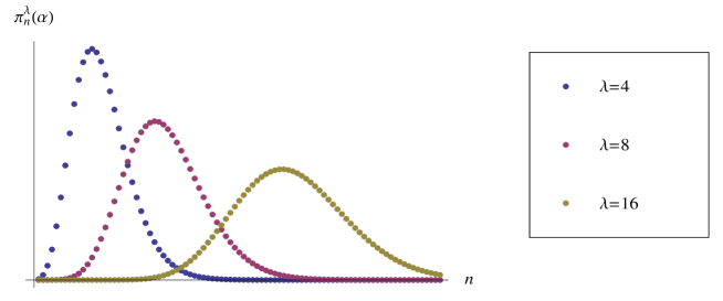
Figure 1: Probability $\pi_{n}^{\lambda}(\alpha)$ for fixed $\alpha=0.8$ and different values of $\lambda$

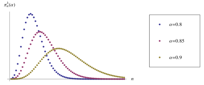
Figure 2: Probability $\pi_{n}^{\lambda}(\alpha)$ for fixed $\lambda=4$ and different values of $\alpha$

Furthermore, inside each energy level ${E}_{n}^{\lambda}$, the allowed angular momenta $j=[0,1/2],\dots,n/2$ appear with different (unnormalized) probabilities:

$$f_{n,j}^{\lambda}(\alpha)\equiv\frac{(2j+1)^{2}}{\lambda-1}\binom{\frac{n}{2}-j+\lambda-2}{\lambda-2}\binom{\frac{n}{2}+j+\lambda-1}{\lambda-2}\alpha^{2n}.$$ (44)

Actually, the distribution function $\pi_{n}^{\lambda}(j)\equiv f_{n,j}^{\lambda}(\alpha)/f_{n}^{\lambda}(\alpha)$, which is independent of $\alpha$, has a maximum for a given $j=j_{0}(n,\lambda)$, with $j_{0}(n,\lambda)$ an increasing sequence of $n$ and decreasing on $\lambda$ (see Figure 3).

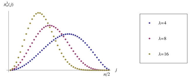
Figure 3: Probability $\pi_{n}^{\lambda}(j)$ for different values of $\lambda$

4.4 Entropy, temperature and ¿maximal acceleration?

Note that, deriving the partition function ${\cal Z}(\alpha)$ and mean energy ${\cal E}(\alpha)$ from the distribution function (41,42) does not involve any thermal (but just pure quantum mechanical) input. In the same way, we can also compute the entropy as a logarithmic measure of the density of states. In fact, denoting by $p_{n}(\alpha)=\alpha^{2n}/{\cal Z}(\alpha)$ the probability of finding our “Einstein solid” in the energy level $n$ with degeneracy $W_{\lambda}(n)$, the entropy can be calculated as

$${\cal S}(\alpha) = -\sum_{n=0}^{\infty}W_{2\lambda}(n)p_{n}(\alpha)\ln p_{n}(\alpha)$$ (45)

$$= -\sum_{n=0}^{\infty}\tbinom{2\lambda+n-1}{n}(1-\alpha^{2})^{2\lambda}\alpha^{2n}\ln((1-\alpha^{2})^{2\lambda}\alpha^{2n})$$

$$= -(1-\alpha^{2})^{2\lambda}\left(\sum_{n=0}^{\infty}\tbinom{2\lambda+n-1}{n}\alpha^{2n}\ln((1-\alpha^{2})^{2\lambda})+\sum_{n=0}^{\infty}\tbinom{2\lambda+n-1}{n}\alpha^{2n}\ln(\alpha^{2n})\right)$$

$$= -(1-\alpha^{2})^{2\lambda}\left(2\lambda\ln(1-\alpha^{2})\sum_{n=0}^{\infty}\tbinom{2\lambda+n-1}{n}\alpha^{2n}+2\ln(\alpha)\sum_{n=1}^{\infty}\tbinom{2\lambda+n-1}{n}n\alpha^{2n}\right),$$

$$= -2\lambda\left(\frac{\alpha^{2}\ln(\alpha^{2})}{1-\alpha^{2}}+\ln(1-\alpha^{2})\right),$$

where we have identified the partition function ${\cal Z}(\alpha)$ and its derivative $\alpha^{2}\frac{d}{d(\alpha^{2})}{\cal Z}(\alpha)$ in the last two summations. Again, there is not any thermal input up to now. If we wanted to assign an “effective” temperature ${\cal T}$ to our “accelerated ensemble”, we could use the universal thermodynamic expression (derivative of the energy with respect to the entropy):

$${\cal T}=\frac{d{\cal E}(\alpha)}{d{\cal S}(\alpha)}=-\frac{1}{\ln(\alpha^{2})},$$ (46)

given in unities of the Einstein temperature $T_{E}$ previously introduced (i.e. ${\cal T}=T/T_{E}$).. The equality (46) can be inverted to formula (40), giving the announced derivation of the assignment (40) from first thermodynamic principles. One could still check consistency (if desired) with other classical formulas relating mean energy and entropy to the partition function, namely:

$${\cal E}(\alpha)=-\frac{d\ln{\cal Z}(\alpha)}{d\beta},\;\;{\cal S}(\alpha)=\frac{d}{d{\cal T}}({\cal T}\ln{\cal Z}(\alpha)),\;\beta\equiv 1/{\cal T}.$$ (47)

A hurried analysis of the relation $\alpha^{2}=e^{-1/{\cal T}}$ would lead to think of the existence of a “maximal acceleration” $\alpha^{2}=1$ (in dimensionless unities). Actually, in the process towards the calculation of thermodynamical quantities, we have made use of a rescaling of the original acceleration $C=c_{\mu}\sigma^{\mu}$, in the expression (36), to ${\cal C}=D^{-1}C=\alpha_{\mu}\sigma^{\mu}$. We can find the relation between $c_{\mu}$ and $\alpha_{\mu}$ as follows. Taking int account that $\varphi^{00}_{00}$ is normalized and the representation (24) is unitary (see Appendix C and Proposition 5.2 of [24]), we know that the accelerated ground state (36) is also normalized. This means that the normalizing global factor $\det(D)^{-\lambda}$ in (36) is related to the partition function ${\cal Z}({\cal C})$ in (37) by:

$$\det(DD^{\dagger})^{-\lambda}=1/{\cal Z}({\cal C})=\det(I-{\cal C}^{{\dagger}}{\cal C})^{\lambda}\Rightarrow\det(DD^{\dagger})=\frac{1}{\det(I-{\cal C}^{{\dagger}}{\cal C})}.$$ (48)

Therefore, for $C=c\sigma^{3}$ and ${\cal C}=\alpha\sigma^{3}$, the relation ${\cal C}^{\dagger}{\cal C}=C^{\dagger}(DD^{\dagger})^{-1}C$ reads:

$$\alpha^{2}=\frac{c^{2}}{1+c^{2}}\Rightarrow c^{2}=\frac{\alpha^{2}}{1-\alpha^{2}}.$$ (49)

With this identification, the mean energy ${\cal E}=\lambda+2\lambda\frac{\alpha^{2}}{1-\alpha^{2}}=\lambda+2\lambda c^{2}$ turns out to be a quadratic function of the acceleration $c$. The dependence of $c$ with the effective temperature ${\cal T}$ is then:

$$c=\sqrt{\frac{e^{-1/{\cal T}}}{1-e^{-1/{\cal T}}}}=\sqrt{{\cal T}}+O(\frac{1}{\sqrt{{\cal T}}})\,\,{\rm for}\,\,{\cal T}>>1.$$ (50)

This behavior departs from the Unruh’s formula (1) even in the limit of high temperatures.

We have seen that the fact that $\alpha$ is bounded is just due to a rescaling of $c$, so that there is not a maximal acceleration in our model as such. Nevertheless, we would like to comment on other arguments in the literature supporting the existence of a bound $a_{\rm max}$ for proper accelerations. One was given time ago in Ref. [34] in connection with conformal kinematics; there the authors analyzed the physical interpretation of the singularities, $1+2cx+c^{2}x^{2}=0$, of the SCT (2). When applying the transformation to an extended object of size $\ell$, an upper-limit to the proper acceleration, $a_{\rm max}\simeq v^{2}/\ell$, is shown to be necessary in order to the tenets of special relativity not to be violated (see [34] for more details). Before, Caianiello [35] derived the existence and physical consequences of a maximal acceleration connected with the Born’s Reciprocity Principle (BPR) [36, 37]. Indeed, one can deduce the existence of a maximal acceleration from the positivity of the Born’s line element

$$d\tilde{\tau}^{2}=dx_{\mu}dx^{\mu}+\frac{\ell^{4}_{\rm min}}{\hbar^{2}}dp_{\mu}dp^{\mu}=d\tau\sqrt{1-\frac{|a^{2}|}{a^{2}_{\rm max}}}$$ (51)

where $d\tau^{2}\equiv dx_{\mu}dx^{\mu}$ and $dp_{\mu}/d\tau\equiv md^{2}x_{\mu}/d\tau^{2}=ma_{\mu}$, as usual. An adaptation of the BRP to the conformal relativity has been put forward by some of us in [20], where a conformal analogue of the line element (51) in the phase space $\mathbb{D}_{4}$ has been considered. However, the existence of a maximal acceleration inside the conformal group does not seem to be apparent neither from this conformal adaptation of the BRP.

In the last years, many papers have been published (see e.g. [38] and references therein), each one introducing the maximal acceleration starting from different motivations and from different theoretical schemes. Among the large list of physical applications of Caianiello’s model we would like to point out the one in cosmology which avoids an initial singularity while preserving inflation. Also, a maximal-acceleration relativity principle leads to a variable fine structure “constant” [38], according to which it could have been extremely small (zero) in the early Universe and then all matter in the Universe could have emerged via the Unruh effect. Moreover, in a non-commutative geometry setting [39], the non-vanishing commutators (72) can be seen as a sign of the granularity (non-commutativity) of space-time in conformal-invariant theories, along with the existence of a minimal length $\ell_{\rm min}$ or, equivalently, a maximal acceleration $a_{\rm max}=v^{2}/\ell_{\rm min}$.

5 Second-Quantized Theory, Conformal Zero Modes and Poincaré $\theta$-vacua

We have discussed the effect of relativistic accelerations in first quantization. However, the proper setting to analyze radiation effects is in the second-quantized theory. Let us denote (for space-saving notation) by $n=\{j,m,q_{1},q_{2}\}$ the multi-index of the one-particle basis wavefunctions $\varphi_{n}$ in (25) and by $\hat{a}_{n}$ (resp. $\hat{a}^{\dagger}_{n}$) operators annihilating (resp. creating) a particle in the state $|n\rangle$. As for the case of a single bosonic mode in (32), an orthonormal basis for the Hilbert space of the second-quantized theory is constructed by taking the orbit through the conformal vacuum $|{0}\rangle$ of the creation operators $\hat{a}^{\dagger}_{n}$:

$$|q(n_{1}),\dots,q(n_{p})\rangle\equiv\frac{(\hat{a}^{\dagger}_{n_{1}})^{q(n_{1})}\dots(\hat{a}^{\dagger}_{n_{p}})^{q(n_{p})}}{(q(n_{1})!\dots q(n_{p})!)^{1/2}}|{0}\rangle,$$ (52)

where $q(n)\in\mathbb{N}$ denotes the occupation number of the state $n$ with energy $2j+2m$.

The fact that the ground state of the first quantization, $\varphi_{0}$, is invariant under Poincaré transformations (remember the discussion after (35)), implies that the annihilation operator $\hat{a}_{0}$ of zero-(“dark”)-energy modes commutes with all Poincaré generators. It also commutes with all annihilation operators and creation operators of particles with positive (“bright”) energy,

$$[\hat{a}_{0},\hat{a}_{n}^{\dagger}]=0,\;n\not=0.$$ (53)

Therefore, by Schur’s Lemma, $\hat{a}_{0}$ must behave as a multiple of the identity when conformal symmetry is broken/restricted to Poincaré symmetry. This means that we can choose Poincaré-invariant vacua $|\theta\rangle$ as being eigenstates of $\hat{a}_{0}$, namely:

$$\hat{a}_{0}|\theta\rangle=\theta|\theta\rangle\Rightarrow{|\theta\rangle=e^{\theta\hat{a}^{\dagger}_{0}-\bar{\theta}\hat{a}_{0}}|0\rangle},$$ (54)

which implies that Poincaré “$\theta$-vacua” $|\theta\rangle$ are (canonical) coherent states of conformal zero modes (remember the general definition in Eq. (33)). Unlike the conformal vacuum $|0\rangle$, which is invariant under the whole conformal group, Poincaré $\theta$-vacua $|\theta\rangle$ are not stable under special conformal transformations (accelerations). In fact, the second-quantized version of (36), for an acceleration ${\cal C}=\alpha\sigma^{3}$ along the third axis, is given by the transformation of annihilation (resp. creation) operators:

$$\tilde{\hat{a}}_{0}=\sum_{n=0}^{\infty}\varphi_{n}(\alpha)\hat{a}_{n}.$$ (55)

We shall assume that $\sum_{n}|\varphi_{n}(\alpha)|^{2}=1$ (normalized probabilities) so that this transformation preserves the original commutation relations $[\tilde{\hat{a}}_{0},\tilde{\hat{a}}_{0}^{\dagger}]=1$. Therefore, accelerated Poincaré $\theta$-vacua are:

$$|\tilde{\theta}\rangle=e^{\theta\tilde{\hat{a}}^{\dagger}_{0}-\bar{\theta}\tilde{\hat{a}}_{0}}|0\rangle,$$ (56)

which can also be written as

$$|\tilde{\theta}\rangle=e^{\theta\sum_{n=1}^{\infty}\overline{\varphi_{n}(\alpha)}\,\tilde{\hat{a}}^{\dagger}_{n}}|\theta\rangle.$$ (57)

We can think of conformal zero modes as “virtual particles” without “bright” energy and undetectable by inertial observers. However, from an accelerated frame, they become “visible” to a Poincaré observer. The average number of particles with energy $E_{n}$ in the accelerated vacuum (56) is then given by

$$N_{n}(\alpha)=\langle\tilde{\theta}|\hat{a}^{\dagger}_{n}\hat{a}_{n}|\tilde{\theta}\rangle=|\theta|^{2}|\varphi_{n}(\alpha)|^{2},$$ (58)

where $|\theta|^{2}$ is the total average number of particles in $|\theta\rangle$, and $|\varphi_{n}(\alpha)|^{2}$ is the occupation number of the energy level $E_{n}$ of the accelerated vacuum $|\tilde{\theta}\rangle$. The situation resembles that in many condensed-matter systems (like Bose-Einstein condensates, superconductors, etc), where one also finds non-empty, coherent ground states.

In the same way, the probability $P_{n}(q,\alpha)$ of observing $q$ particles with energy $E_{n}$ in $|\tilde{\theta}\rangle$ can be calculated as:

$$P_{n}(q,\alpha)=|\langle q(n)|\tilde{\theta}\rangle|^{2}=\frac{e^{-|\theta|^{2}}}{q!}|\theta|^{2q}\,|\varphi_{n}(\alpha)|^{2q}=\frac{e^{-|\theta|^{2}}}{q!}N_{n}^{q}(\alpha).$$ (59)

Therefore, the relative probability of observing a state with total energy $E$ in the excited vacuum $|\tilde{\theta}\rangle$ is:

$$P(E)=\sum_{\begin{array}[]{c}q_{0},\dots,q_{k}:\\ \sum^{k}_{n=0}E_{n}q_{n}=E\end{array}}\prod^{k}_{n=0}P_{n}({q}_{n},\alpha)\,.$$ (60)

For the case studied in this paper, this distribution function can be factorized as $P(E)=\Omega(E)e^{-E/{\cal T}}$, where $\Omega(E)$ is a relative weight proportional to the number of states with energy $E$ and the factor $e^{-E/{\cal T}}$ fits this weight properly to a temperature ${\cal T}$.

One can also compute the total mean energy

$${E}(\alpha)=\langle\tilde{\theta}|\sum_{n=1}^{\infty}E_{n}\hat{a}^{\dagger}_{n}\hat{a}_{n}|\tilde{\theta}\rangle=|\theta|^{2}\sum_{n=1}|\varphi_{n}(\alpha)|^{2}E_{n}=|\theta|^{2}{\cal E}(\alpha),$$ (61)

which, as expected, is the product of ${\cal E}(\alpha)$ by the average number of particles $|\theta|^{2}$ in $|\theta\rangle$. The free parameter $|\theta|^{2}$ is also linked to a vacuum (“dark”) energy $E_{0}=|\theta|^{2}{\cal E}_{0}=|\theta|^{2}\lambda$ whose value should be determined by experiments, just like, for example, the cosmological constant. Like other non-zero vacuum expectation values, zero-point energy leads to observable consequences as, for instance, the Casimir effect, and influences the behavior of the Universe at cosmological scales, where the vacuum (dark) energy is expected to contribute to the cosmological constant, which affects the expansion of the universe (see e.g. [40] for a nice review). Actually, dark energy is the most popular way to explain recent observations that the universe appears to be expanding at an accelerating rate.

6 Comments and Outlook

As already commented in the Introduction, conformal field theories also seem to provide a universal description of low-energy black hole thermodynamics, which is only fixed by symmetry arguments (see [12, 13] and references therein). Actually, Unruh’s temperature (1) coincides with Hawking’s temperature

$$T=\frac{\hbar v^{3}}{8\pi Mk_{B}G}=\frac{2\pi GM\hbar}{\Sigma vk_{B}}$$ (62)

($\Sigma=4\pi r_{g}^{2}=8\pi G^{2}M^{2}/v^{4}$ stands for the surface of the event horizon) when the acceleration is that of a free falling observer on the surface $\Sigma$, i.e. $a=v^{4}/(4GM)=GM/r_{g}^{2}$. Here, the Virasoro algebra proves to be a physically important subalgebra of the gauge algebra of surface deformations that leave the horizon fixed for an arbitrary black hole. Thus, the fields on the surface must transform according to irreducible representations of the Virasoro algebra, which is the general symmetry principle that governs the density of microscopic states. Bekenstein-Hawking expression for the entropy can be then calculated from the Cardy formula [41, 42] (see also [43] for logarithmic corrections). Therefore, in the Hawking effect, the calculation of thermodynamical quantities, linked to the statistical mechanical problem of counting microscopic states, is reduced to the study of the representation theory of the conformal group.

Although our approach to the quantum analysis of accelerated frames shares with the previous description of black hole thermodynamics the existence of an underlying conformal invariance, we should not confuse both schemes. Conformal invariance in Hawking effect manifests itself as an infinite-dimensional gauge algebra of (two-dimensional) surface deformations. However, the infinite-dimensional character of conformal symmetry seems to be an exclusive patrimony of two-dimensional physics, and conformal invariance in (3+1)-dimensions is finite-(15)-dimensional, thus accounting for transitions to uniformly accelerated frames only. To account for higher-order effects of gravity on quantum field theory from a group-theoretical point of view, one should consider more general diffeomorphism (Lie) algebras. Higher-dimensional analogies of the infinite two-dimensional conformal symmetry have been proposed by us in [14, 15, 11, 16, 17]. We think that these inifinite ${\cal W}$-like symmetries can play some fundamental role in quantum gravity models, as a gauge guiding principle.

To conclude, we would also like to mention that, the same spontaneous $SU(2,2)$-symmetry breaking mechanism explained in this paper applies to general $SU(N,M)$-invariant quantum theories, where an interesting connection between “curvature and statistics” has emerged [44, 45]. We hope that many more interesting physical phenomena remain to be unraveled inside conformal-invariant quantum (field) theory.

Appendix A Vacuum radiation as a consequence of space-time mutilation

The existence of event horizons in passing to accelerated frames of reference leads to unitarily inequivalent representations of the quantum field canonical commutation relations and to a (in-)definition of particles depending on the state of motion of the observer.

To use an explicit example, let us consider a real scalar massless field $\phi(x)$, satisfying the Klein-Gordon equation

$$\eta^{\mu\nu}\partial_{\mu}\partial_{\nu}\phi(x)=0\,.$$ (63)

Let us denote by $a_{k},a^{*}_{k}$ the Fourier coefficients of the decomposition of $\phi$ into positive and negative frequency modes:

$$\phi(x)=\int dk(a_{k}f_{k}(x)+a^{*}_{k}f^{*}_{k}(x)).$$ (64)

The Fourier coefficients $a_{k},a^{*}_{k}$ are promoted to annihilation and creation operators $\hat{a}_{k},\hat{a}^{*}_{k}$ of particles in the quantum field theory. The Minkowski vacuum $|0\rangle_{M}$ is defined as the state nullified by all annihilation operators

$$\hat{a}_{k}|0\rangle_{M}=0,\;\forall k.$$ (65)

Let us consider now the Rindler coordinate transformation (see e.g. [2]):

$$t=a^{-1}e^{az^{\prime}}\sinh(at^{\prime}),\;\;z=a^{-1}e^{az^{\prime}}\cosh(at^{\prime}).$$ (66)

The worldline $z^{\prime}=0$ has constant acceleration $a$ (in natural unities). This transformation entails a mutilation of Minkowski spacetime into patches or charts with event horizons.

The new coordinate system provides a new decomposition of $\phi$ into Rindler positive and negative frequency modes:

$$\phi(x^{\prime})=\int dq(a^{\prime}_{q}f^{\prime}_{q}(x^{\prime})+a^{\prime*}_{q}f^{\prime*}_{q}(x^{\prime})).$$ (67)

The Rindler vacuum $|0\rangle_{R}$ is defined as the state nullified by all Rindler annihilation operators:

$$\hat{a}^{\prime}_{q}|0\rangle_{R}=0\,\forall q.$$ (68)

One can see that the Minkowski vacuum $|0\rangle_{M}$ and the Rindler vacuum $|0\rangle_{R}$ are not identical. Actually, the Minkowski vacuum $|0\rangle_{M}$ has a nontrivial content of Rindler particles. In fact, the Fourier components $a^{\prime}_{q},{a^{\prime}}^{*}_{q}$ of the field $\phi$ in the new (accelerated) reference frame are expressed in terms of both $a_{k},a^{*}_{k}$ through a Bogolyubov transformation:

$$a^{\prime}_{q}=\int{dk\left(\alpha_{qk}a_{k}+\beta_{qk}a^{*}_{k}\right)}\,,$$

$$\alpha_{qk}=\langle f^{\prime}_{q}|f_{k}\rangle,\;\;\beta_{qk}=\langle f^{\prime}_{q}|f^{*}_{k}\rangle.$$ (69)

The vacuum states $|0\rangle_{M}$ and $|0\rangle_{R}$, defined by the conditions (65) and (68), are not identical if the coefficients $\beta_{qk}$ in (69) are not zero. In this case the Minkowski vacuum has a non-zero average number of Rindler particles given by:

$$N_{R}=\langle 0|\hat{N}_{R}|0\rangle_{M}=\langle 0|\int dq\hat{a}^{\prime{\dagger}}_{q}\hat{a}^{\prime}_{q}|0\rangle_{M}=\int{dkdq|\beta_{qk}|^{2}}.$$ (70)

That is, both quantizations are inequivalent.

Appendix B Conformal particles from constrained nonlinear $\sigma$-models on SU(2,2)

Let us briefly report on a $G_{0}\equiv SL(2,\mathbb{C})\times\mathbb{R}^{+}$ (Lorentz times dilations) gauge-invariant Lagrangian approach (of sigma-model type) to the formulation of conformal $G=SU(2,2)$ invariant quantum particles, with the cotangent of $G$ as a preliminary phase space. This formulation has been thoroughly developed in Reference [20], where we used a generalized Dirac method for the quantization of constrained systems, which resembles in some aspects the standard approach to quantizing coadjoint orbits of a group $G$ (see e.g. classical References as [46], [47] and [48]).

Denote by $g(t)\in G$ trajectories on $G$, $\vartheta^{L}\equiv-ig^{-1}dg=-ig^{-1}\dot{g}dt$ the left-invariant Maurer-Cartan one-form and $\Gamma$ the hermitian form in Eq. (11). Then the singular action

$$A(g,\dot{g})=\int{\rm tr}(\Gamma\vartheta^{L})$$ (71)

is naturally left-$G$-invariant under rigid transformations $g(t)\to g^{\prime}g(t),\forall g^{\prime}\in G$, the infinitesimal generators of this symmetry (right-invariant vector fields) being the basic operators/observables of the first-quantized theory. In addition, the action (71) is also right-$G_{0}$-invariant under local-gauge transformations $g(t)\to g(t)g_{0}(t),\;\forall g_{0}(t)\in G_{0}$ (see [20] for a proof). At the quantum level, the $G_{0}$ gauge right-invariance of the proposed Lagrangian manifests itself by leaving complex wave functions on $G$, $\phi:G\to\mathbb{C}$, right-invariant under gauge-group $G_{0}$ transformations, i.e. $\phi(gg_{0})=\phi(g),\forall g_{0}\in G_{0},g\in G$. Actually, the last strict invariant condition, $\phi(gg_{0})=\phi(g)$, can be relaxed to “invariance up to a phase”, $\phi(gg_{0})=u_{l}(g_{0})\phi(g),u_{s}(g_{0})\in U(1)$, thus allowing internal degrees of freedom, like the spin $l=s$, to enter the theory ($l$ denotes any label characterizing the representation). The “Gauss-law-like” constraints related to this $G_{0}$ gauge right-invariance are written in terms of the corresponding infinitesimal generators (left-invariant ‘$L$’ vector fields) $M_{\mu\nu}^{L}$ and $D^{L}$ of Lorentz and dilation transformations as: $M_{\mu\nu}^{L}\phi=0$ (for spin-less $s=0$ particles) and $D^{L}\phi=\lambda\phi$ (for conformal, scale or mass dimension $\lambda$), respectively. These constraints restrict the support of wave functions $\phi$ from $G$ to the eight-dimensional domain $\mathbb{D}_{4}=G/G_{0}$ of the complex Minkowski (phase) space $\mathbb{C}^{4}$. An extra condition $K_{\mu}^{L}\phi=0$ is just intended to select the “position” (versus “momenta”) representation and it is necessary for irreducibility of the quantum representation. The last condition further restricts the support of $\phi$ to $\mathbb{R}^{4}$. This means that Cauchy hypersurfaces have dimension four. In other words, the time-translations generator $P_{0}$ is now a dynamical operator, on an equal footing with spatial-translations generators $P_{j}$, thus suffering Heisenberg indeterminacy relations too. This fact can also be inferred from the generalized Klein-Gordon equation $C_{2}^{L}\phi=m_{00}^{2}\phi$, with $C^{L}_{2}$ the quadratic conformal Casimir (6) (which has the same expression in terms of left-invariant generators as in terms of right-invariant ones) and $m_{00}^{2}=\lambda(\lambda+4)$ (indeed, use the constraints $M_{\mu\nu}^{L}\phi=0$, $K_{\mu}^{L}\phi=0$ and $D^{L}\phi=\lambda\phi$ and the last commutation relation in (5)). In fact, let us consider the alternative (vector and pseudo-vector) combinations

$$\tilde{P}_{\mu}\equiv\frac{1}{2}(P_{\mu}+K_{\mu}),\;\;\tilde{K}_{\mu}\equiv\frac{1}{2}(P_{\mu}-K_{\mu}),$$

with new commutation relations:

$$\left[\tilde{P}_{\mu},\tilde{K}_{\nu}\right]=\eta_{\mu\nu}D,\;\left[\tilde{P}_{\mu},\tilde{P}_{\nu}\right]=M_{\mu\nu},\;\left[\tilde{K}_{\mu},\tilde{K}_{\nu}\right]=-M_{\mu\nu},$$ (72)

in terms of which the Casimir (6) reads

$$C_{2}=D^{2}-\frac{1}{2}M_{\mu\nu}M^{\mu\nu}+\tilde{P}_{\mu}\tilde{P}^{\mu}-\tilde{K}_{\mu}\tilde{K}^{\mu}.$$ (73)

A new compatible set of constraints are: $M_{\mu\nu}^{L}\phi=0$ and $\tilde{K}^{L}_{\mu}\phi=0$, resulting in wave functions $\phi(g)$, having support on the extended Minkowski space $G/{\cal P}\simeq\mathbb{R}^{4}\times\mathbb{R}^{+}$. The commutator $[D^{L},\tilde{K}^{L}_{\mu}]=-\tilde{P}^{L}_{\mu}$ now precludes the imposition of $D^{L}\phi=\lambda\phi$ (otherwise we would be forced to impose $\tilde{P}^{L}_{\mu}\phi=0$ too and the representation would be trivial). Instead, the Casimir constraint

$$C_{2}^{L}\phi=m_{00}^{2}\phi\Rightarrow((D^{L})^{2}+(\tilde{P}^{L})^{2})\phi=m_{00}^{2}\phi$$ (74)

can be compatibly imposed, togheter with $M_{\mu\nu}^{L}\phi=0$ and $\tilde{K}^{L}_{\mu}\phi=0$, thus leading to the announced generalized Klein-Gordon equation with $D$ playing the role of the new (proper) time evolution generator.

References

- [1] P.C.W. Davies, Scalar production in Schwarzschild and Rindler metrics, J. Phys. A: Math. Gen. 8 (1975) 609-616
- [2] N. D. Birrell and P. C. W. Davies, Quantum Fields in Curved Space, Cambridge Monographs on Mathematical Physics (1994).
- [3] S.A. Fulling, Nonuniqueness of Canonical Field Quantization in Riemannian Space-Time, Phys. Rev. D7 (1973) 2850-2862
- [4] W. G. Unruh, Notes on black-hole evaporation, Phys. Rev. D14 (1976) 870
- [5] S.W. Hawking, Black-hole explosions?, Nature 248 (1974) 30
- [6] R. F. Bishop and A. Vourdas, Generalised coherent states and Bogoliubov transformations, J. Phys. A: Math. Gen. 19 (1986) 2525-2536.
- [7] E. L. Hill, On accelerated coordinate systems in classical and relativistic mechanics, Phys. Rev. 67 (1945) 358-363.
- [8] L. J. Boya and J. M. Cerveró, Contact Transformations and Conformal Group. I. Relativistic Theory, International Journal of Theoretical Physics 12 (1975) 47-54
- [9] T. Fulton, F. Rohrlich and L. Witten, Physical consequences to a coordinate transformation to a uniformly accelerationg frame, Nuovo Cimento 26 (1962) 652-671
- [10] V. Aldaya, M. Calixto and J.M. Cerveró, Vacuum Radiation and Symmetry Breaking in Conformally Invariant Quantum Field Theory, Commun. Math. Phys. 200 (1999) 325-354
- [11] M. Calixto, Higher-U(2,2)-spin fields and higher-dimensional W-gravities: quantum AdS space and radiation phenomena, Class. Quantum Grav. 18 (2001) 3857-3884
- [12] S. Carlip, Entropy from Conformal Field Theory at Killing Horizons, Class. Quant. Grav. 16 (1999) 3327-3348
- [13] I. Agullo, J. Navarro-Salas, G. J. Olmo, L. Parker, Hawking radiation by Kerr black holes and conformal symmetry, Phys. Rev. Lett. 105 (2010) 211305
- [14] M. Calixto, Structure constants for new infinite-dimensional Lie algebras of tensor operators and applications, J. Phys. A33 (2000) L69-L75
- [15] M. Calixto, Promoting finite to infinite symmetries: the 3+1 analogue of the Virasoro algebra and higher-spin fields, Mod. Phys. Lett. A15 (2000) 939-944
- [16] M. Calixto, Generalized higher-spin algebras and symbolic calculus on flag manifolds, J. Geom. Phys. 56 (2006) 143-174
- [17] V. Aldaya, J.L. Jaramillo, Extended diffeomorphism algebras in (quantum) gravitational physics, Int. J. Mod. Phys. A18 (2003) 5795
- [18] A.O. Barut and R.B. Haugen, Theory of the Conformally Invariant Mass, Ann. Phys. 71 (1972) 519-541
- [19] G. Mack, All Unitary Ray Representations of the Conformal Group SU(2,2) with Positive Energy, Commun. Math. Phys. 55 (1977) 1-28
- [20] M. Calixto and E. Pérez-Romero, Conformal Spinning Quantum Particles in Complex Minkowski Space as Constrained Nonlinear Sigma Models in and Born’s Reciprocity, Int. J. Geom. Meth. Mod. Phys. 8 (2011) 587-619. arXiv:1006.5958
- [21] C.W. Misner, K.S. Thorne and J.A. Wheeler, Gravitation, Freeman, San Francisco (1973)
- [22] H. Weyl, Space, Time and Matter, Dover. NY. First Edition 1922
- [23] H.A. Kastrup, Gauge properties of the Minkowski space, Phys. Rev. 150, 1183 (1966)
- [24] M. Calixto and E. Pérez-Romero, Extended MacMahon-Schwinger’s Master Theorem and Conformal Wavelets in Complex Minkowski Space, Appl. Comput. Harmon. Anal. 21 (2006) 204-229, arXiv:1002.3498
- [25] W. Rühl, Field Representations of the Conformal Group with Continuous Mass Spectrum, Commun. Math. Phys. 30 (1973) 287-302
- [26] V. Aldaya and J.A. de Azcárraga: Group manifold analysis of the structure of relativistic quantum dynamics, Annals of Physics 165 (1985) 484-504
- [27] S. Fubini, A.J. Hanson and R. Jackiw: New approach to field theory, Phys. Rev. D7 (1973) 1732-1760
- [28] A. Perelomov, Generalized Coherent States and Their Apllications, Springer-verlag (1986)
- [29] J.R. Klauder and Bo-Sture Skagerstam: Coherent States: Applications in Physics and Mathematical Physics, World Scientific (1985)
- [30] S.T. Ali, J-P. Antoine, J.P. Gazeau, Coherent States, Wavelets and Their Generalizations, Springer (2000)
- [31] Philip M. Morse, Thermal Physics, W.A. Benjamin 1969
- [32] J. Cariñena, M. A. del Olmo and M. Santander, Kinematic groups and dimensional analysis, J. Phys. A: Math. Gen. 14 (1981) 1-14
- [33] J. Cariñena, M. A. del Olmo and M. Santander, A new look at dimensional analysis from a group theoretical viewpoint, J. Phys. A: Math. Gen. 18 (1985) 1855-1872
- [34] W.R. Wood, G. Papini and Y.Q. Cai, Conformal transformations and maximal acceleration, Il Nuovo Cimento 104 (1989) 653-663
- [35] E.R. Caianiello, Is there a maximal aceleration?, Lettere al Nuovo Cimento 32 (1981) 65-70
- [36] M. Born, A suggestion for unifying quantum theory and relativity, Proc. R. Soc. A165 (1938) 291-302
- [37] M. Born, Reciprocity theory of elementary particles, Rev. Mod. Phys. 21 (1949) 463-473
- [38] C. Castro, On the variable fine structure constant, strings and maximal-acceleration phase space relativity, International Journal of Modern Physics A18 (2003) 5445-5473
- [39] J. Madore, An Introduction to Noncommutative Differential Geometry and its Physical Applications, 2nd ed., London Mathematical Society Lecture Note Series, 257 Cambridge Univ. Press. 1999
- [40] G.E. Volovik: Vacuum energy: myths and reality, Int. J. Mod. Phys. D15 (2006) 1987-2010
- [41] J.A. Cardy, Operator content of two-dimensional conformally invariant theories, Nucl. Phys. B270 (1986) 186-204
- [42] H.W.J. Blöte, J.A. Cardy and M.P. Nightingale, Conformal invariance, the central charge, and universal finite-size amplitudes at criticality, Phys. Rev. Lett. 56 (1986) 742-745
- [43] S. Carlip, Logarithmic Corrections to Black Hole Entropy from the Cardy Formula, Class. Quant. Grav. 17 (2000) 4175-4186
- [44] M. Calixto and V. Aldaya, Curvature, zero modes and quantum statistics, J. Phys. A39 (2006) L539-L545
- [45] M. Calixto and V. Aldaya, Thermal Vacuum Radiation in Spontaneously Broken Second-Quantized Theories on Curved Phase Spaces of Constant Curvature, Int. J. Geom. Meth. Mod. Phys. 6 (2009) 513-531
- [46] B. Kostant, Quantization and unitary representations, Lecture Notes in Math. 170, Springer-Verlag, Berlin-Heidelberg-New York, 1970
- [47] A. A. Kirillov, Elements of the Theory of Representations, Springer-Verlag, Berlin, 1976.
- [48] A.P. Balachandran, G. Marmo, B-S. Skagerstan and A. Stern, Gauge Theories and Fiber Bundles: Applications to Particle Dynamics, Lecture Notes in Physics 188, Springer-Verlag, Berlin, 1983