Spin dephasing and pumping in graphene due to random spin-orbit interaction

Abstract

We consider spin effects related to the random spin-orbit interaction in graphene. Such a random interaction can result from the presence of ripples and/or other inhomogeneities at the graphene surface. We show that the random spin-orbit interaction generally reduces the spin dephasing (relaxation) time, even if the interaction vanishes on average. Moreover, the random spin-orbit coupling also allows for spin manipulation with an external electric field. Due to the spin-flip interband as well as intraband optical transitions, the spin density can be effectively generated by periodic electric field in a relatively broad range of frequencies.

I Introduction

Graphene is currently attracting much attention as a new excellent material for modern electronics novoselov04 ; novoselov05 ; geim07 . The natural two-dimensionality of graphene matches perfectly to the dominating planar technology of other semiconducting materials, and correspondingly gives the way to creating new hybrid systems. However, the most striking properties of graphene are not directly related to its two-dimensionality. Due to the bandstructure effects, electrons in pure graphene can be described by the relativistic Dirac Hamiltonian, leading to the linear electron energy spectrum near the Dirac points. As a result, the electronic and transport properties of graphene are significantly different from those of any other metallic or semiconducting material,geim07 ; neto09 ; peres09 ; rakyta except (to some extent) its parent material – the clean graphite.graphite

It has been also suggested that graphene may have good perspectives as a new material for applications in spintronics.nishioka07 ; cho07 ; guimaraes10 ; yazyev10 The intrinsic spin-orbit interaction in graphene is usually very small, and therefore one can expect extremely long spin dephasing (relaxation) time. hernando06 ; min06 ; yao07 ; gmitra09 ; nanotubes Thus, spin injected to graphene, for instance from ferromagnetic contacts, can maintain its coherence for a relatively long time. Experiments demonstrate spin relaxation times for various graphene-based systems spanned over several orders of magnitudetombros07 ; tombros08 ; maassen ; yang ; han with some of them being much shorter than expected.tombros07 ; tombros08 The reason of this contradiction is not quite clear, and several different explanations of these observations have been already put forward.hernando07 ; ertler09 ; zhou10 In this paper we present another model based on the random Rashba spin-orbit interaction.sherman03 ; glazov05 Physical origin of such random spin-orbit interaction can be related to the ripples existing at the surface of graphene meyer07 ; ishigami07 ; wehling08 and/or to some impurities adsorbed at the surface, which randomly enhance the magnitude of spin-orbit coupling as compared to that in the clean graphene.ertler09

One of the key issues in spintronics (including graphene-based spintronics) is the possibility of spin manipulation with an external electric/optical field. This includes spin generation, spin rotation, spin switching, etc. Here we consider the possibility of spin pumping in graphene using the idea of combined resonance in systems with Rashba spin-orbit interaction.rashba61 ; rashba03 The possibility of spin manipulation using optical excitationzaharchenya is based on various mechanisms of spin-orbit interaction in semiconductor systems. In particular, the spin polarization appears in systems with regular spin-orbit coupling, subject to periodic electric field. tarasenko06 ; raichev07 ; khomitsky It has been shown recently, that the random spin-orbit interaction also can be applied to generate spin polarization in symmetric semiconductor quantum wells. dugaev09 In this paper we show that similar method can be used to generate spin polarization in graphene with random Rashba spin-orbit interaction. To do this we analyze the intensity of optically-induced spin-flip transitions assuming two-dimensional massless Dirac model of electron energy spectrum in graphene, and calculate the magnitude of spin-polarization induced by the optical pumping.

The paper is structured as follows. In section 2 we describe the model Hamiltonian assumed for graphene. Spin dephasing due to the random spin-orbit Rashba coupling is calculated in section 3. In turn, spin pumping by an external electric field is considered in section 4. Final conclusions are presented in section 5.

II Model

To describe electrons and holes in the vicinity of Dirac points we use the model Hamiltonian $\mathcal{H}_{0}$ which is sufficient when considering the effects related to low-energy electron and hole excitations. We also include the spin-dependent perturbation in the form of a spatially fluctuating Rashba spin-orbit interaction, $\mathcal{H}_{\rm so}$. Thus, the system Hamiltonian can be written as (we use system of units with $\hbar\equiv 1$)

$$\mathcal{H}=\mathcal{H}_{0}+\mathcal{H}_{\rm so},$$ (1)

$$\mathcal{H}_{0}=v\,\mbox{\boldmath$\tau$}\cdot\mathbf{k},$$ (2)

$$\mathcal{H}_{\rm so}=\frac{\lambda(\mathbf{r})}{v}\,\left(\frac{\partial\mathcal{H}_{0}}{\partial k_{x}}\sigma_{y}-\frac{\partial\mathcal{H}_{0}}{\partial k_{y}}\sigma_{x}\right)$$

$$=\lambda(\mathbf{r})\,\left(\tau_{x}\sigma_{y}-\tau_{y}\sigma_{x}\right),$$ (3)

where $v$ is the electron velocity, $\lambda(\mathbf{r})$ is the random spin-orbit parameter, $\mathbf{r}=(x,y)$ is the two-dimensional coordinate, and $\tau$ and $\sigma$ are the Pauli matrices acting in the sublattice and spin spaces, respectively.kane05 Equations (2) and (3) show that spin-orbit coupling can be described by a conventional Rashba Hamiltonian, proportional to $v_{x}\sigma_{y}-v_{y}\sigma_{x}$, where the velocity components $v_{x},v_{y}$ are, in general, obtained with the unperturbed Hamiltonian $\mathcal{H}_{0}$. It is well known that there is an intrinsic (internal) spin-orbit coupling in graphene, which is related to relativistic corrections to the crystal field of the corresponding lattice. In addition, a spatially uniform Rashba field can be induced by the substrate on which the graphene sheet is located. The reported results suggest that these interactions, which can be considered as independent sources of spin relaxation, are either very weak gmitra09 ; gold or do not contribute to the dephasing rate by symmetry reasons.zhou10 Therefore, we will neglect them in our considerations and will briefly discuss their role in the following.

The Schrödinger equation, $(\mathcal{H}_{0}-\varepsilon)\,\psi_{\mathbf{k}}=0$, for the pseudospinor components of the wavefunction $\psi_{\mathbf{k}}$ is

$$\left(\begin{array}[]{cc}-\varepsilon&vk_{-}\\ vk_{+}&-\varepsilon\end{array}\right)\left(\begin{array}[]{c}\varphi_{\mathbf{k}}\\ \chi_{\mathbf{k}}\end{array}\right)=0,$$ (4)

where $k_{\pm}=k_{x}\pm ik_{y}$. The normalized solutions corresponding to the eigenstates $\varepsilon_{k}=\pm vk$ of Hamiltonian $\mathcal{H}_{0}$ can be written in the form

$$\psi_{\mathbf{k}\sigma\pm}(\mathbf{r})=\frac{e^{i\mathbf{k}\cdot\mathbf{r}}}{\sqrt{2}}\left(\left|1\sigma\right\rangle\pm\frac{k_{+}}{k}\left|2\sigma\right\rangle\right),$$ (5)

where the $\pm$ signs correspond to the states in upper and lower branches, respectively.

We assume that the average value of spin-orbit interaction vanishes, while the spatial fluctuation of $\lambda(\mathbf{r})$ can be described by the correlation function $F\left(\mathbf{r-r}^{\prime}\right)$ of a certain form,

$$\left\langle\lambda(\mathbf{r})\right\rangle=0,$$ (6)

$$C(\mathbf{r}-\mathbf{r^{\prime}})\equiv\langle\lambda(\mathbf{r})\,\lambda(\mathbf{r}^{\prime})\rangle=\left\langle\lambda^{2}\right\rangle F\left(\mathbf{r-r}^{\prime}\right).$$ (7)

When calculating spin dephasing, one can consider only the electron states corresponding to the upper branch (conduction band) of the energy spectrum, $\varepsilon_{k}=vk$. The spin-flip scattering from the random potential determines the spin relaxation in this particular band, while from symmetry of the system follows that spin dephasing in the lower (valence) band is the same. The intraband matrix elements of the random spin-orbit interaction (3) in the basis of wavefunctions (5) for the conduction band form the following matrix in the spin subspace

$$V_{\mathbf{kk^{\prime}}}=\lambda_{\mathbf{kk^{\prime}}}\left(\begin{array}[]{cc}0&-ik_{-}/k\\ ik_{+}^{\prime}/k^{\prime}&0\end{array}\right),$$ (8)

where $\lambda_{\mathbf{kk^{\prime}}}$ is the Fourier component of the random spin-orbit coupling. Since scattering from the random spin-orbit potential is elastic, only the intraband transitions contribute to the spin relaxation.

III Spin dephasing

To demonstrate how the random spin-orbit coupling works in graphene and how its effects can be observed in experiment, as well as to compare graphene and conventional two-dimensional semiconductor structures, we calculate in this Section the corresponding spin dephasing time. For this purpose we use the kinetic equation for the density matrix (Wigner distribution function), tarasenko06_2 ; dugaev09

$$\frac{\partial\rho_{\mathbf{k}}}{\partial t}=\mathrm{St}\,\rho_{\mathbf{k}}.$$ (9)

The collision integral $\mathrm{St}\,\rho_{\mathbf{k}}$ on the right-hand side of this equation is due to the spin-flip scattering from the random spin-orbit interaction,

$$\mathrm{St}\,\rho_{\mathbf{k}} = \pi\sum_{\mathbf{k^{\prime}}}\left(2V_{\mathbf{kk^{\prime}}}\rho_{\mathbf{k^{\prime}}}V_{\mathbf{k^{\prime}k}}-V_{\mathbf{kk^{\prime}}}V_{\mathbf{k^{\prime}k}}\rho_{\mathbf{k}}-\rho_{\mathbf{k}}V_{\mathbf{kk^{\prime}}}V_{\mathbf{k^{\prime}k}}\right)$$ (10)

$$\times\delta\left(\varepsilon_{\mathbf{k}}-\varepsilon_{\mathbf{k^{\prime}}}\right).$$

We assume the following form of the density matrix:

$$\rho_{\mathbf{k}}=\rho_{0k}+s_{\mathbf{k}}\sigma_{z},$$ (11)

where the first term $\rho_{0k}$ corresponds to the spin-unpolarized equilibrium state. On substituting (8) and (11) into Eq. (10) we find

$$\mathrm{St}\,\rho_{\mathbf{k}}=-2\pi\sigma_{z}\sum_{k^{\prime}}C(\mathbf{q})\left(s_{\mathbf{k}}+s_{\mathbf{k^{\prime}}}\right)\,\delta\left(\varepsilon_{\mathbf{k}}-\varepsilon_{\mathbf{k^{\prime}}}\right),$$ (12)

where $C(\mathbf{q})\equiv\left\langle\lambda_{\mathbf{kk^{\prime}}}^{2}\right\rangle$ and $\mathbf{q}=\mathbf{k^{\prime}-k}$. Assuming that $s_{\mathbf{k}}$ does not depend on the point at the Fermi surface we obtain

$$\mathrm{St}\,\rho_{\mathbf{k}}=-\frac{4k\sigma_{z}s_{k}}{\pi v}\int_{0}^{2k}\frac{C(\mathbf{q})}{\sqrt{4k^{2}-q^{2}}}dq.$$ (13)

For definiteness, we assume that the characteristic spatial range of the random spin-orbit fluctuations is $R$, and take $C(\mathbf{q})$ in the following form:

$$C(\mathbf{q})=2\pi\langle\lambda^{2}\rangle R^{2}e^{-qR},$$ (14)

satisfying the normalization condition

$$\int C(\mathbf{q})\frac{d^{2}q}{(2\pi)^{2}}=\langle\lambda^{2}\rangle.$$ (15)

The resulting spin relaxation rate is not strongly sensitive to the shape of the correlator. However, the applicability of the approach based on Eq.(12) depends on the ratio of electron mean free path $\ell$ to $R$, being valid only if $\ell/R\gg 1$. In such a case, typically realized in graphene, the electron spin experiences indeed random, weakly correlated in time fluctuations of the spin-orbit coupling. In addition, we can safely neglect the effect of the random spin-orbit coupling on the momentum relaxation rate. Finally, for the spin dephasing time we obtain the following expression:

$$\frac{1}{\tau_{k}^{s}} = \frac{8k}{v}\left\langle\lambda^{2}\right\rangle R^{2}\int_{0}^{2kR}\frac{e^{-x}dx}{\sqrt{4k^{2}R^{2}-x^{2}}}$$ (16)

$$= \frac{4\pi k}{v}\left\langle\lambda^{2}\right\rangle R^{2}\left[I_{0}(2kR)-L_{0}(2kR)\right],$$

where $I_{0}(x)$ and $L_{0}(x)$ are the modified Bessel and Struve functions of zeroth order, respectively.

Figure 1: Spin dephasing time as a function of the characteristic range $R$ of the random spin-orbit fluctuations.

In the limiting semiclassical ($kR\gg 1$) and quantum ($kR\ll 1$) cases we find

$$\frac{1}{\tau_{k}^{s}}\simeq\frac{4R}{v}\left\langle\lambda^{2}\right\rangle\left\{\begin{array}[]{cc}1,&kR\gg 1,\\ \\ \pi kR,&kR\ll 1.\end{array}\right.$$ (17)

For $kR\gg 1$, the result in Eq.(17) can be interpreted as the special realization of the Dyakonov-Perel’ spin relaxation mechanism. To see this, we note that the electron spin rotates at the rate $\Omega\sim\left\langle\lambda^{2}\right\rangle^{1/2}$, with the precession direction changing randomly at the timescale of the order of time that electron needs to pass through one domain of the size $R$, i.e., $\tau_{R}\sim R/v.$ The resulting spin relaxation rate $1/\tau_{k}^{s}$ is of the order of $\Omega^{2}\tau_{R}.$ It is worth mentioning that at given spatial and energy scale of the fluctuating spin-orbit field, the decrease in the electron free path and in the momentum relaxation time leads to the decrease in the spin dephasing rate: if $\ell\ll R$, electron spin interacts with the local rather than with the rapidly changing random field, and spin relaxation rate becomes of the order of $\left<\lambda^{2}\right>\tau$, where $\tau$ is the momentum relaxation time. This agrees qualitatively with the observations of Ref.[yang, ], however, a quantitative comparison needs a more detailed analysis.

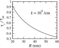
Taking examples with typical values $v=10^{8}$ cm/s, $R\sim 50$ nm, and $\langle\lambda^{2}\rangle\sim 500$ $\mu$eV², similar to what can be expected from Ref.[hernando06, ], we obtain $\tau_{k}^{s}$ less than or of the order of 10 ns. As one can see from Eq.(17), the spin relaxation for small $kR\ll 1$ is suppressed, as can be understood in terms of the averaging of the random field over a large $1/k^{2}\gg R^{2}$ area. The full $k$-dependence in Eq.(17) implies that the spin dephasing rate is proportional to $n^{1/2}$ at low carrier concentrations $n$ and is independent of $n$ at higher ones. Therefore, at the charge neutrality point, where $n=0$, the spin relaxation vanishes, in agreement with the observations of Ref.[han, ]. Moreover, our approach qualitatively agrees with the increase in the spin relaxation time in the bilayer graphene compared to the single layer one han : the transverse rigidity of the bilayer can be larger, thus suppressing formation of the long-range ripples, and, as a result, the random spin-orbit coupling.

Equation (17) shows that, as far as the spin dephasing is considered, the only difference between graphene and conventional semiconductors sherman03 ; glazov05 ; dugaev09 is related to the fact that the electron velocity is constant for the former case and is proportional to the momentum in the latter one. As we will see in the next Section, this difference becomes crucial for the spin pumping processes.

The dependence of spin relaxation time, calculated from Eq. (16) as a function of the characteristic domain size $R$ of the random spin-orbit interaction is presented in Fig. 1, were $\tau_{s0}$ is defined as $\tau_{s0}^{-1}\equiv 8\left\langle\lambda^{2}\right\rangle/vk$. The curves corresponding to different values of $k>10^{6}$ cm^-1 would be practically indistinguishable in this figure.

Here several comments on the numerical values of spin relaxation are in order. The values observed in experiments on spin injection from ferromagnetic contactstombros07 ; tombros08 are of the order of 10^-10 s, two orders of magnitude less than our estimate which does not take into account explicitly the role of the Si-based substrates. The effect of the SiO₂ substrate, including the contributions from impurities and electron-phonon coupling, was thoroughly analyzed in Ref.[ertler09, ]. However, the obtained dephasing rates were well below the experimental values and also below the estimate obtained here, leading the authors of Ref.[ertler09, ] to the suggestion of an important role of heavy adatoms in the spin-orbit coupling.adatoms On the other hand, it was shown that the spin dephasing rate can be strongly influenced at relatively high temperatures by the electron-electron collisions.zhou10 However, including these collisions does not bring theoretical values closer to the experimental ones.

The discrepancies between theory and experiment and between experimental data obtained on different systems call for a more detailed analysis of the experimental situation, including the dependence of spin relaxation time on the device functional properties and the experimental techniques applied.

IV Spin pumping

Let us consider now spin pumping by an external electromagnetic periodic field corresponding to the vector potential $\mathbf{A}(t)$. We assume that the system described by Eqs. (1)-(3) is additionally in a constant magnetic field $\mathbf{B}$. For simplicity, we consider the Voigt geometry with the field in the graphene plane, so that the effects of Landau quantization are absent. Thus, the Hamiltonian $\mathcal{H}_{0}$ includes now the constant field and can be written as

$$\mathcal{H}_{0}=v\,\mbox{\boldmath$\tau$}\cdot\mathbf{k}+\Delta\sigma_{x},$$ (18)

where $2\Delta=g\mu_{B}B$ is the spin splitting and the magnetic field is oriented along the $x-$axis (the electron Landé factor for graphene is $g=2$). The induced spin polarization is opposite to the direction of the magnetic field.

Since we are interested in real transitions in which the energy is conserved, we consider interaction with a single component of the periodic electromagnetic field, $\mathbf{A}(t)=\mathbf{A}e^{-i\omega t},$ which enters in the gauge-invariant form

$$\mathcal{H}_{A}=-\frac{e}{c}\,\frac{\partial\mathcal{H}}{\partial\mathbf{k}}\cdot\mathbf{A}(t)=-\frac{ev}{c}\,\mbox{\boldmath$\tau$}\cdot\mathbf{A}(t),$$ (19)

and in the following we treat the term $\mathcal{H}_{A}$ as a small perturbation.

The absorption in a periodic field (probability of field-induced transitions in unit time) can be written as

$$I(\omega)=\mathrm{Re\,Tr}\sum_{\mathbf{k}}\int\frac{d\varepsilon}{2\pi}\;\mathcal{H}_{A}\;G_{\mathbf{k}}(\varepsilon+\omega)\;\mathcal{H}_{A}\;G_{\mathbf{k}}(\varepsilon),$$ (20)

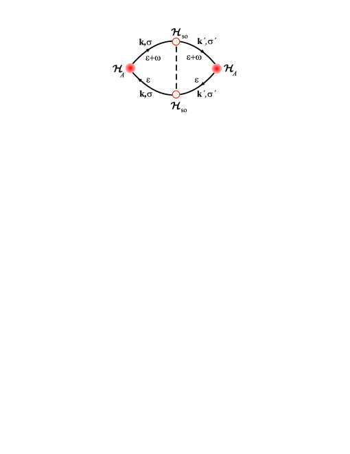
where $G_{\mathbf{k}}(\varepsilon)$ is the Green function. In the absence of spin-orbit interaction, the absorption (20) does not include any spin-flip transitions. We can account for the spin-orbit interaction (3) in the second order perturbation theory, including the corresponding matrix elements as shown in Fig. 2. This means that we do not consider perturbation terms as the self-energy within a single Green function assuming that they are already included in the electron relaxation rate.

Figure 2: (Color online.) Feynman diagrams for the light absorption in the second order perturbation theory with respect to the random spin-orbit interaction. The coupling and electromagnetic vertices are shown as white and filled circles, respectively.

Thus, in the second order perturbation theory with respect to the random spin-orbit interaction $\mathcal{H}_{\rm so}$ we obtain

$$I(\omega) = \mathrm{Re\,Tr}\,\sum_{\mathbf{kk^{\prime}}}\int\frac{d\varepsilon}{2\pi}\;\mathcal{H}_{A}\;G_{\mathbf{k}}^{0}(\varepsilon+\omega)\;\mathcal{H}_{\rm so}^{\mathbf{kk^{\prime}}}\,G_{\mathbf{k^{\prime}}}^{0}(\varepsilon+\omega)\;$$ (21)

$$\times\mathcal{H}_{A}\;G_{\mathbf{k^{\prime}}}^{0}(\varepsilon)\;\mathcal{H}_{\rm so}^{\mathbf{k^{\prime}k}}\;G_{\mathbf{k}}^{0}(\varepsilon),$$

where Green’s function $G_{\mathbf{k}}^{0}(\varepsilon)=\mathrm{diag}\left\{G_{\mathbf{k}\uparrow}^{0}(\varepsilon),\,G_{\mathbf{k}\downarrow}^{0}(\varepsilon)\right\}$ corresponds to the Hamiltonian $\mathcal{H}_{0}$ of Eq. (18),

$$G_{\mathbf{k}\sigma}^{0}(\varepsilon)=\frac{\varepsilon+v\,\mbox{\boldmath$\tau$}\cdot\mathbf{k}+\Delta\sigma+\mu}{\left(\varepsilon-\varepsilon_{1k\sigma}+\mu+i\delta\,\mathrm{sgn}\,\varepsilon\right)\left(\varepsilon-\varepsilon_{2k\sigma}+\mu+i\delta\,\mathrm{sgn}\,\varepsilon\right)},$$ (22)

with $\sigma=\pm 1$ corresponding to the spins oriented along and opposite to the $x-$axis, respectively, $\varepsilon_{(1,2)k\sigma}=\pm v\,k+\Delta\sigma$, $\delta$ being the half of the momentum relaxation rate, $\delta=1/2\tau$, and $\mu$ denoting the chemical potential.

Figure 3: (Color online.) The energy spectrum and indirect spin-flip transitions in graphene in a uniform magnetic field $\mathbf{B}$. Long and short arrows correspond to the interband and intraband transitions, respectively.

Diagrams in Fig. 2 show the qualitative difference between the graphene and semiconductor quantum well with respect to the effects of random spin-orbit coupling. In semiconductors, the external electric field is explicitly coupled to the anomalous spin-dependent term in the electron velocity, which is random, and therefore the diagrams describing the corresponding transitions include only two Green functions. In graphene, due to the absence of randomness-originated term in the Hamiltonian $\mathcal{H}_{A},$ four Green functions are required to take into account the random contribution of the spin-orbit coupling. This situation, in some sense, is more close to what is observed in the conventional kinetic theory of normal metal conductivity, where the coupling to the external field does not depend on the randomness explicitly, and the additional disorder effects appear due to the self-energy and/or due to the vertex corrections, as in Fig. 2.

Upon calculating contributions from the diagrams of Fig. 2, one finds the total rate of spin-flip and spin-conserving transitions due to the random spin-orbit coupling in the form

$$I_{\rm rso}(\omega) = \frac{e^{2}A^{2}}{c^{2}}\,\mathrm{Re\,Tr}\sum_{\sigma\sigma^{\prime}}\sum_{\mathbf{kk^{\prime}}}v^{2}C(\mathbf{q})\int\frac{d\varepsilon}{2\pi}(\mbox{\boldmath$\tau$}\cdot\mathbf{n}_{A})$$ (23)

$$\times G_{\mathbf{k}\sigma}^{0}(\varepsilon+\omega)\tau_{-}G_{\mathbf{k^{\prime}}\sigma^{\prime}}^{0}(\varepsilon+\omega)(\mbox{\boldmath$\tau$}\cdot\mathbf{n}_{A})$$

$$\times G_{\mathbf{k^{\prime}}\sigma^{\prime}}^{0}(\varepsilon)\,\tau_{+}G_{\mathbf{k}\sigma}^{0}(\varepsilon),$$

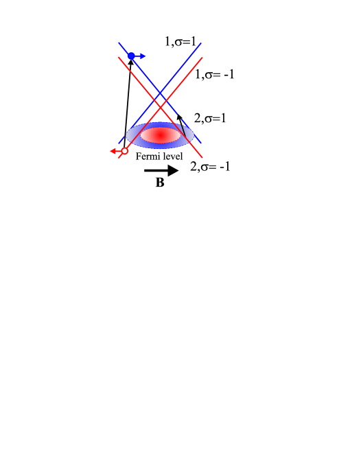
where $\tau_{\pm}=\tau_{{}_{x}}\pm i\tau_{y},$ and $\mathbf{n}_{A}$ describes the direction of $\mathbf{A}$. In the following we assume linear polarization of light, $\mathbf{A}=(A,\,0)$. After calculating the trace and integrating over energy $\varepsilon$ in Eq. (23) one finds a rather cumbersome expression (see Appendix) consisting of several terms, each of them corresponding to transitions between certain branches of the spectrum (Fig. 3). For definiteness, we locate the chemical potential in the valence band. Correspondingly, only the transitions from the bands $(2\,\uparrow)$ and $(2\,\downarrow)$ to the unoccupied states in the bands $(1\,\uparrow)$, $(1\,\downarrow)$, $(2\,\uparrow)$ and $(2\,\downarrow)$ are possible. We will concentrate on the optically induced spin-flip transitions contributing to the optically-generated spin pumping. Hence, we do not consider spin-conserved transitions contributing to the usual Drude conductivity.Kuzmenko ; optics ; ESR

IV.1 Interband spin-flip transitions

Figure 4: (Color online.) The parameter $K_{2\downarrow}(\omega)$ for the rate of the spin-flip interband transitions in the high-frequency domain (a) and $K_{2\uparrow}$ (b) for different values of the range parameter $R$ describing characteristic size of the fluctuations in spin-orbit interaction and $\langle\lambda^{2}\rangle=100$ $\mu$eV².

Let us consider first the spin-flip transitions from the valence to conduction bands, such as $\overline{\mathbf{k}}_{2}\rightarrow$ $\overline{\mathbf{k}}_{1}^{\prime}.$ For convenience we introduce the parameter $\overline{\mathbf{k}}_{j}=\left(\mathbf{k,\sigma}_{x}\right)_{j},$ describing the momentum and spin projection for an electron in the subband $j.$ The corresponding expression for the transition rate can be obtained from the equations presented in the Appendix, and considerably simplified by taking into account that: (i) in the nonsingular terms $\varepsilon_{\overline{\mathbf{k}}_{1}}-\varepsilon_{\overline{\mathbf{k}}_{2}}$ can be substituted by $\omega,$ (ii) in the semiclassical limit $kR\gg 1$ the energy change due to the change in the momentum is small compared to $1/\tau$, and (iii) the photon energy is much larger than the characteristic low-energy scale parameters, i.e., $\omega\gg 1/\tau,$ and $\omega\gg\Delta$. We mention that the linear in $\Delta$ terms have to be kept despite $\Delta\ll\omega$ since the resulting spin pumping rate, determined by the contributions of both initial spin states, is linear in $\Delta$. The expressions for the parameters $K_{2\sigma}(\omega)$, which determine the spin-flip rate as introduced in the Appendix, Eq.(31), can be then simplified, and as a result one obtains the following formula for the spin-flip rate in the relevant frequency domain:

$$I_{2\sigma\to 1\sigma^{\prime}}(\omega)=4\pi\sigma\frac{e^{2}A^{2}}{c^{2}}\frac{v^{4}}{\omega}\sum_{\mathbf{kk^{\prime}}}C\left(\mathbf{q}\right)\left[f(\varepsilon_{\overline{\mathbf{k}}_{2}})-f(\varepsilon_{\overline{\mathbf{k}}_{1}^{\prime}})\right]$$

$$\times\frac{k^{2}-kq\cos\varphi}{\varepsilon_{\overline{\mathbf{k}}_{2}}+\omega-\varepsilon_{\overline{\mathbf{k}}_{1}}}\,\frac{\delta\left(\varepsilon_{\overline{\mathbf{k}}_{2}}+\omega-\varepsilon_{\overline{\mathbf{k}}_{1}^{\prime}}\right)}{\left(\varepsilon_{\overline{\mathbf{k}}_{2}}+\omega-\varepsilon_{\overline{\mathbf{k}}_{2}^{\prime}}\right)\left(\varepsilon_{\overline{\mathbf{k}}_{2}}-\varepsilon_{\overline{\mathbf{k}}_{2}^{\prime}}\right)}\,.\hskip 5.69046pt$$ (24)

The transitions are constrained due to the $\delta$-function in Eq. (24) corresponding to the energy conservation with the change in the momentum $\mathbf{q}$ (here we use $\varphi=\cos^{-1}(\mathbf{k},\mathbf{q})$)

$$\delta\left(\varepsilon_{\overline{\mathbf{k}}_{2}}+\omega-\varepsilon_{\overline{\mathbf{k}}_{1}^{\prime}}\right)=\frac{|\omega-vk-2\sigma\Delta|\;\delta(\varphi-\varphi_{0})}{v^{2}kq\,|\sin\varphi_{0}|}\,,$$ (25)

where $\varphi_{0}$ is a solution of the equation

$$vk+2\sigma\Delta-\omega+v\sqrt{k^{2}-2kq\cos\varphi+q^{2}}=0,$$ (26)

which gives us the condition for a minimum value of momentum in Eq. (26), $vk_{\min}=\omega-2\sigma\Delta$. The energy conservation determines the angle $\varphi_{0}$ between the vectors $\mathbf{k}$ and $\mathbf{q}$ as

$$\cos\varphi_{0}=\frac{q}{2k}+\frac{\omega-2\sigma\Delta}{vq}\left(1-\frac{\omega-2\sigma\Delta}{2vk}\right).$$ (27)

The usual condition of $|\cos\varphi_{0}|<1$ leads to the following restrictions in the integration over $q$ in Eq. (24):

Figure 5: (Color online.) The parameter $K_{2}(\omega)\equiv K_{2\downarrow}(\omega)-K_{2\uparrow}(\omega)$ for the spin injection rate for different $R$. Other parameters are the same as Fig.4.

a) if $\omega/2-\sigma\Delta<vk<\omega-2\sigma\Delta$ then $vk-|vk+2\sigma\Delta-\omega|<vq<vk+|vk+2\sigma\Delta-\omega|$,

b) if $\omega/2-\sigma\Delta>vk$ then $-vk+|vk+2\sigma\Delta-\omega|<vq<vk+|vk+2\sigma\Delta-\omega|$.

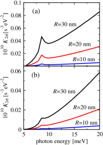
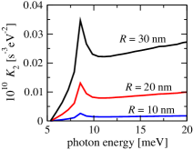
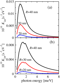
Accounting for all these conditions, the integral over $k$ and $q$ in Eq. (24) can be calculated numerically. We used the following parameters: $\mu=-3$ meV, corresponding to the Fermi momentum $k_{F}\approx 5\times 10^{4}$ cm^-1 and hole concentration $\approx 4\times 10^{8}$ cm^-2, $\Delta=1$ meV, and $1/\tau=1$ meV. These parameters correspond to a rather clean graphene and strong Zeeman splitting of the bands (magnetic field of 17 T). For numerical accuracy, the calculations were performed with exact Eqs.(33) and (35). The results of numerical calculations for the interband spin-flip transitions are presented in Fig. 4. Figure 5 presents the quantity describing the total spin injection rate for the interband transitions in this frequency domain, $K_{2}(\omega)\equiv K_{2\downarrow}(\omega)-K_{2\uparrow}(\omega)$. The positive sign of $K_{2}(\omega)$ corresponds to the fact that the absolute value of spin density decreases due to the pumping. The peaks correspond to the absorption edge of direct optical transitions, where the transition probability rapidly increases, and the increase at large frequencies is due to the linear energy dependence of the density of states.

IV.2 Intraband transitions in the hole subband

Using the general formulas (33) and (35) we can write down the expression for the spin-flip intraband transitions within the valence band in a low-frequency region $\omega\ll\left|\mu\right|$. Such transitions are associated with a relatively large change of the momentum in the absorption process, and one can expect that they give a smaller transition rate. Upon taking into account that $\varepsilon_{\overline{\mathbf{k}}_{1}}-\varepsilon_{\overline{\mathbf{k}}_{2}}=-2\mu\gg\omega,$ and $\left|\varepsilon_{\overline{\mathbf{k}}_{2}}-\varepsilon_{\overline{\mathbf{k}}_{2}^{\prime}}\right|\ll\left|\mu\right|$, we find

$$I_{2\sigma\to 2\sigma^{\prime}}(\omega)=-4\pi\sigma\frac{e^{2}A^{2}}{c^{2}}\frac{v^{4}\tau^{2}}{\mu^{2}(1+\omega^{2}\tau^{2})}$$

$$\times\sum_{\mathbf{kk^{\prime}}}C\left(\mathbf{q}\right)\left[f(\varepsilon_{\overline{\mathbf{k}}_{2}})-f(\varepsilon_{\overline{\mathbf{k}}_{2}^{\prime}})\right]$$

$$\times\varepsilon_{\overline{\mathbf{k}}_{2}}\varepsilon_{\overline{\mathbf{k}}_{2}^{\prime}}(k^{2}-kq\cos\varphi)\,\frac{\delta\left(\varepsilon_{\overline{\mathbf{k}}_{2}}+\omega-\varepsilon_{\overline{\mathbf{k}}_{2}^{\prime}}\right)}{(\varepsilon_{\overline{\mathbf{k}}_{2}}+\omega-\varepsilon_{\overline{\mathbf{k}}_{1}^{\prime}})(\varepsilon_{\overline{\mathbf{k}}_{2}}-\varepsilon_{\overline{\mathbf{k}}_{1}^{\prime}})}.$$ (28)

The $\delta$-function can be presented in the form of Eq.(25), where $\varphi_{0}$ is a solution of the equation

$$vk+2\sigma\Delta-\omega-v\sqrt{k^{2}-2kq\cos\varphi+q^{2}}=0.$$ (29)

Figure 6: (Color online.) The parameter $K_{2\downarrow}(\omega)$ for the rate of the spin-flip intraband transitions in the low-frequency domain (a) and $K_{2\uparrow}(\omega)$ (b) for different values of the range parameter $R$. Other parameters are the same as Fig.4.

Figure 7: (Color online.) The parameter $K_{2}(\omega)\equiv K_{2\downarrow}(\omega)-K_{2\uparrow}(\omega)$ for the spin injection rate for different $R$ in the low-frequency domain. Other parameters are the same as Fig.4. Unmarked line corresponds to $R=30$ nm.

Equations (29) and (26) are similar, with the important difference in the sign in front of $\sqrt{k^{2}-2kq\cos\varphi+q^{2}}.$ In the case of interband transitions this corresponds to the transitions occurring at $\omega\approx 2vk,$ while the intraband transitions occur at lower frequencies determined by the possible momentum transfer due to the randomness of the spin-orbit coupling. The solution exists only for $vk>\omega-2\sigma\Delta$ and gives Eq.(27). However, the condition $|\cos\varphi_{0}|<1$ leads here to a different restriction. Since only the condition $\omega-2\sigma\Delta<2vk$ is consistent with $vk>\omega-2\sigma\Delta$, the momentum $q$ should be then in the single range of $vk-|vk+2\sigma\Delta-\omega|<vq<vk+|vk+2\sigma\Delta-\omega|$, in contrast to the case of interband transitions.

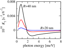
The results of calculations for the intraband transitions are presented in Fig. 6. The intensity of such processes is relatively small compared to the interband transitions, and they can be seen only at low photon energies. Figure 7 corresponds to spin injection rate by the intraband transitions, $K_{2}(\omega)$.

V Conclusions

We have considered certain spin effects associated with random spin-orbit interaction in graphene. First, we have calculated the corresponding spin relaxation time, and believe that this mechanism can be dominating when the amplitude of fluctuations in spin-orbit interaction is large enough. This may happen in the presence of surface ripples with short wavelengths. The other possibility can be related to the absorbed impurities at both surfaces of a free-standing graphene. One can expect especially strong random spin-orbit coupling for heavy impurity atoms.

The second effect concerns the possibility of spin pumping by an external electromagnetic field. The results of our calculations show that graphene can be used as a material, in which the electron spin density can be generated by the optical pumping. The mechanism of pumping here is related to the spin-flip transitions associated with the random Rashba spin-orbit interaction.

Appendix A Formula for the absorption rate

Using (22) and (23), after calculating the trace and integrating over energy $\varepsilon$, we find out that spin-flip processes can be characterized by the initial state as $I_{1\downarrow}(\omega),I_{2\downarrow}(\omega),I_{1\uparrow}(\omega),$ and $I_{2\uparrow}(\omega)$ with the corresponding transition rate $I_{j\sigma}(\omega)$ defined as

$$I_{j\sigma}(\omega) \equiv \frac{16e^{2}A^{2}}{c^{2}}K_{j\sigma}(\omega),$$ (30)

$$K_{j\sigma}(\omega) \equiv -\mathrm{Im}\int v^{4}C\left(\mathbf{q}\right)\frac{J_{j\sigma}(\mathbf{q,}\omega)}{\omega+i\delta}\frac{d^{2}kd^{2}k^{\prime}}{\left(2\pi\right)^{4}},$$ (31)

describing transitions from the band and spin states corresponding to the subscript $j\sigma$. Here $J_{j\sigma}(\mathbf{q,}\omega)$ have the form:

$$J_{1\downarrow}(\mathbf{q,}\omega) = \left.\left[f(\varepsilon_{1k\downarrow})-f(\varepsilon_{1k\downarrow}+\omega)\right]\,\frac{(\varepsilon_{1k\downarrow}^{2}-\Delta^{2}+\varepsilon_{1k\downarrow}\omega)(k^{2}-kq\cos\varphi)}{(\varepsilon_{1k\downarrow}-\varepsilon_{1k^{\prime}\uparrow})(\varepsilon_{1k\downarrow}-\varepsilon_{2k\downarrow})(\varepsilon_{1k\downarrow}-\varepsilon_{2k^{\prime}\uparrow})}\right.$$ (32)

$$\times\left.\frac{1}{\left(\varepsilon_{1k\downarrow}+\omega-\varepsilon_{1k^{\prime}\uparrow}+i\delta\right)(\varepsilon_{1k\downarrow}+\omega-\varepsilon_{2k\downarrow}+i\delta)\left(\varepsilon_{1k\downarrow}+\omega-\varepsilon_{2k^{\prime}\uparrow}+i\delta\right)}\right.,$$

$$J_{2\downarrow}(\mathbf{q,}\omega) = \left.\left[f(\varepsilon_{2k\downarrow})-f(\varepsilon_{2k\downarrow}+\omega)\right]\,\frac{(\varepsilon_{2k\downarrow}^{2}-\Delta^{2}+\varepsilon_{2k\downarrow}\omega)(k^{2}-kq\cos\varphi)}{(\varepsilon_{2k\downarrow}-\varepsilon_{2k^{\prime}\uparrow})(\varepsilon_{2k\downarrow}-\varepsilon_{1k\downarrow})(\varepsilon_{2k\downarrow}-\varepsilon_{1k^{\prime}\uparrow})}\right.$$ (33)

$$\times\left.\frac{1}{\left(\varepsilon_{2k\downarrow}+\omega-\varepsilon_{2k^{\prime}\uparrow}+i\delta\right)(\varepsilon_{2k\downarrow}+\omega-\varepsilon_{1k\downarrow}+i\delta)\left(\varepsilon_{2k\downarrow}+\omega-\varepsilon_{1k^{\prime}\uparrow}+i\delta\right)}\right.,$$

$$J_{1\uparrow}(\mathbf{q,}\omega) = \left.\left[f(\varepsilon_{1k\uparrow})-f(\varepsilon_{1k\uparrow}+\omega)\right]\,\frac{(\varepsilon_{1k\uparrow}^{2}-\Delta^{2}+\varepsilon_{1k\uparrow}\omega)(k^{2}-kq\cos\varphi)}{(\varepsilon_{1k\uparrow}-\varepsilon_{1k^{\prime}\downarrow})(\varepsilon_{1k\uparrow}-\varepsilon_{2k\uparrow})(\varepsilon_{1k\uparrow}-\varepsilon_{2k^{\prime}\downarrow})}\right.$$ (34)

$$\times\left.\frac{1}{(\varepsilon_{1k\uparrow}+\omega-\varepsilon_{1k^{\prime}\downarrow}+i\delta)\left(\varepsilon_{1k\uparrow}+\omega-\varepsilon_{2k\uparrow}+i\delta\right)(\varepsilon_{1k\uparrow}+\omega-\varepsilon_{2k^{\prime}\downarrow}+i\delta)}\right.,$$

$$J_{2\uparrow}(\mathbf{q,}\omega) = \left.\left[f(\varepsilon_{2k\uparrow})-f(\varepsilon_{2k\uparrow}+\omega)\right]\,\frac{(\varepsilon_{2k\uparrow}^{2}-\Delta^{2}+\varepsilon_{2k\uparrow}\omega)(k^{2}-kq\cos\varphi)}{(\varepsilon_{2k\uparrow}-\varepsilon_{2k^{\prime}\downarrow})(\varepsilon_{2k\uparrow}-\varepsilon_{1k\uparrow})(\varepsilon_{2k\uparrow}-\varepsilon_{1k^{\prime}\downarrow})}\right.$$ (35)

$$\times\left.\frac{1}{(\varepsilon_{2k\uparrow}+\omega-\varepsilon_{2k^{\prime}\downarrow}+i\delta)\left(\varepsilon_{2k\uparrow}+\omega-\varepsilon_{1k\uparrow}+i\delta\right)(\varepsilon_{2k\uparrow}+\omega-\varepsilon_{1k^{\prime}\downarrow}+i\delta)}\right..$$

Although the expressions seem to be long, all $J_{j\sigma}(\mathbf{q},\omega)$ terms have the same simple structure. They contain energy-difference denominators corresponding to the transitions from initial $j\sigma$ states to all allowed final states, and the corresponding resonant terms. Here the single allowed spin-conserving transition arising due to the $\mathcal{H}_{A}$ term in Eq.(19) is the momentum-conserving as well, while the two transitions caused by random spin-orbit term $\mathcal{H}_{\mathrm{so}}^{\mathbf{k^{\prime}k}}$ are off-diagonal both in the spin and momentum subspaces, as illustrated in Fig.2. Taking the imaginary part in each of these terms we get $\delta-$functions corresponding to the energy conservation for the transitions to different bands.

References

- (1) K. S. Novoselov, A. K. Geim, S. V. Morozov, D. Jiang, Y. Zhang, S. V. Dubonos, I. V. Grigorieva, and A. A. Firsov, Science 306, 666 (2004).
- (2) K. S. Novoselov, A. K. Geim, S. V. Morozov, D. Jiang, M. I. Katsnelson, I. V. Grigorieva, S. V. Dubonos, and A. A. Firsov, Nature (London) 438, 197 (2005).
- (3) A. K. Geim, K. S. Novoselov, Nature Mater. 6, 183 (2007).
- (4) A. H. Castro Neto, F. Guinea, N. M. R. Peres, K. S. Novoselov, and A. K. Geim, Rev. Mod. Phys. 81, 109 (2009).
- (5) N. M. R. Peres, J. Phys. Condens. Matter 21, 323201 (2009).
- (6) Analysis of the bandstructure in the presence of spin-orbit coupling can be found in P. Rakyta, A. Kormányos, and J. Cserti, Phys. Rev. B 82, 113405 (2010).
- (7) The Dirac-like electron spectrum in single carbon layers was established by P. R. Wallace Phys. Rev. 71, 622 (1947) and observed experimentally in graphite (I. A. Luk’yanchuk and Y. Kopelevich, Phys. Rev. Lett. 93, 166402 (2004)). Also, the quantum Hall effects in graphene and clean graphite are similar: I. A. Luk’yanchuk and Y. Kopelevich, Phys. Rev. Lett. 97, 256801 (2006).
- (8) M. Nishioka and A. M. Goldman, Appl. Phys. Lett. 90, 252505 (2007).
- (9) S. Cho, Y. F. Chen, and M. S. Fuhrer, Appl. Phys. Lett. 91, 123105 (2007).
- (10) F. S. M. Guimarães, A. T. Costa, R. B. Muniz, and M. S. Ferreira, Phys. Rev. B81, 233402 (2010).
- (11) O. V. Yazyev, Rep. Prog. Phys. 73, 056501 (2010).
- (12) D. Huertas-Hernando, F. Guinea, and A. Brataas, Phys. Rev. B74, 155426 (2006).
- (13) H. Min, J. E. Hill, N. A. Sinitsyn, B. R. Sahu, L. Kleinman, and A. H. MacDonald, Phys. Rev. B74, 165310 (2006).
- (14) Y. Yao, F. Ye, X. L. Qi, S. C. Zhang, and Z. Fang, Phys. Rev. B75, 041401(R) (2007).
- (15) M. Gmitra, S. Konschuh, C. Ertler, C. Ambrosch-Draxl, and J. Fabian, Phys. Rev. B80, 235431 (2009).
- (16) Spin relaxation times in carbon nanotubes, which can be considered as the rolled graphene sheets are indeed long enough to allow information transfer (L. E. Hueso, J. M. Pruneda, V. Ferrari, G. Burnell, J. P. Valdés-Herrera, B. D. Simons, P. B. Littlewood, E. Artacho, A. Fert, and N. D. Mathur, Nature 445, 410 (2007)) due to the very weak spin-orbit coupling. However, theoretical analysis shows that the spin resonance caused by external electric field can be observable in these systems: A. De Martino, R. Egger, K. Hallberg, and C. A. Balseiro, Phys. Rev. Lett. 88, 206402 (2002).
- (17) N. Tombros, C. Jozsa, M. Popinciuc, H. T. Jonkman, and B. J. van Wees, Nature (London) 448, 571 (2007).
- (18) N. Tombros, S. Tanabe, A. Veligura, C. Jozsa, M. Popinciuc, H. T. Jonkman, and B. J. van Wees, Phys. Rev. Lett. 101, 046601 (2008).
- (19) T. Maassen, F. K. Dejene, M. H. D. Guimares, C. Józsa, and B. J. van Wees, preprint arXiv:1012.0526.
- (20) T.-Y. Yang, J. Balakrishnan, F. Volmer, A. Avsar, M. Jaiswal, J. Samm, S.R. Ali, A.Pachoud, M. Zeng, M. Popinciuc, G. Güntherodt, B. Beschoten, B. Özyilmaz, preprint arXiv:1012.1156.
- (21) Wei Han and Roland K. Kawakami, preprint arXiv:1012.3435.
- (22) D. Huertas-Hernando, F. Guinea, and A. Brataas, Eur. Phys. J. Special Topics 148, 177 (2007); D. Huertas-Hernando, F. Guinea, and A. Brataas, Phys. Rev. Lett. 103, 146801 (2009).
- (23) C. Ertler, S. Konschuh, M. Gmitra, and J. Fabian, Phys. Rev. B80, 041405(R) (2009).
- (24) Y. Zhou and M. W. Wu, Phys. Rev. B82, 085304 (2010).
- (25) E. Ya. Sherman, Phys. Rev. B67, 161303(R) (2003).
- (26) M. M. Glazov and E. Ya. Sherman, Phys. Rev. B71, 241312(R) (2005).
- (27) J. C. Meyer, A. K. Geim, M. I. Katsnelson, K. S. Novoselov, T. J. Booth, and S. Roth, Nature (London) 446, 60 (2007).
- (28) M. Ishigami, J. H. Chen, W. G. Cullen, M. S. Fuhrer, and E. D. Williams, Nano Lett. 7, 6 (2007).
- (29) T. O. Wehling, A. V. Balatsky, A. M. Tsvelik, M. I. Katsnelson, and A. I. Lichtenstein, EPL 84, 17003 (2008).
- (30) E. I. Rashba and V. I. Sheka, Fizika Tverdogo Tela 3, 2369 (1961 [Sov. Phys. Solid State 3, 1718 (1962)].
- (31) E. I. Rashba and Al. L. Efros, Phys. Rev. Lett. 91, 126405 (2003); Appl. Phys. Lett. 83, 5295 (2003).
- (32) Optical orientation, ed. by F. Mayer and B. Zakharchenya (North-Holland, Amsterdam, 1984).
- (33) S. A. Tarasenko, Phys. Rev. B73, 115317 (2006).
- (34) O. E. Raichev, Phys. Rev. B75, 205340 (2007).
- (35) A. A. Perov, L. V. Solnyshkova, and D. V. Khomitsky, Phys. Rev. B 82, 165328 (2010); D. V. Khomitsky, Phys. Rev. B 79, 205401 (2009).
- (36) V. K. Dugaev, E. Ya. Sherman, V. I. Ivanov, and J. Barnaś, Phys. Rev. B80, 081301(R) (2009).
- (37) C. L. Kane and E. J. Mele, Phys. Rev. Lett. 95, 226801 (2005).
- (38) The influence of the substrate on the spin-orbit coupling is weak for graphene on the top of SiO2 and SiC. An exception is given by graphene on the Ni/Au substrate, where, due to the large atomic number of Au, induced spin-orbit coupling is very strong: A. Varykhalov, J. Sanchez-Barriga, A. M. Shikin, C. Biswas, E. Vescovo, A. Rybkin, D. Marchenko, and O. Rader, Phys. Rev. Lett. 101, 157601 (2008) However, this extreme case is not of our interest here.
- (39) The detailed analysis done by A. H. Castro Neto and F. Guinea, Phys. Rev. Lett. 103, 026804 (2009) shows that taking into account the bond hybridization by the adatoms can lead to the spin relaxation rate of the order of the observed experimentally.
- (40) S. A. Tarasenko, JETP Letters 84, (2006).
- (41) A. B. Kuzmenko, I. Crassee, D. van der Marel, P. Blake, and K. S. Novoselov, Phys. Rev. B 80, 165406 (2009).
- (42) Effects of spin-orbit coupling for the optical properties in disorder-free graphene were considered by P. Ingenhoven, J. Z. Bernád, U. Zülicke, and R. Egger, Phys. Rev. B 81, 035421 (2010)
- (43) Magnetic-field induced electron spin resonance in graphene at frequency was analyzed in B. Dóra, F. Murányi and F. Simon, EPL 92 17002 (2010).