Exotic supersymmetry of the kink-antikink crystal, and the infinite period limit

Abstract

Some time ago, Thies et al. showed that the Gross-Neveu model with a bare mass term possesses a kink-antikink crystalline phase. Corresponding self-consistent solutions, known earlier in polymer physics, are described by a self-isospectral pair of one-gap periodic Lamé potentials with a Darboux displacement depending on the bare mass. We study an unusual supersymmetry of such a second order Lamé system, and show that the associated first order Bogoliubov-de Gennes Hamiltonian possesses the own nonlinear supersymmetry. The Witten index is ascertained to be zero for both of the related exotic supersymmetric structures, each of which admits several alternatives for the choice of a grading operator. A restoration of the discrete chiral symmetry at zero value of the bare mass, when the kink-antikink crystalline condensate transforms into the kink crystal, is shown to be accompanied by structural changes in both of the supersymmetries. We find that the infinite period limit may or may not change the index. We also explain the origin of the Darboux dressing phenomenon recently observed in a non-periodic self-isospectral one-gap Pöschl-Teller system, which describes the Dashen, Hasslacher and Neveu kink-antikink baryons.

1 Introduction

The Gross-Neveu (GN) model [1, 2, 3] is a remarkable (1+1)-dimensional theory of self-interacting fermions that has no gauge fields or gauge symmetries, but exhibits some important features of quantum chromodynamics, namely, asymptotic freedom, dynamical mass generation, and chiral symmetry breaking [4]. It has been widely studied over the years and the richness of its properties is still astonishing. Some time ago, Thies et al. showed that at finite density, the ground state of the model with a discrete chiral symmetry is a kink crystal [5], while the kink-antikink crystalline phase was found in the GN model with a bare mass term [6]. Then, Dunne and Basar derived a new self-consistent inhomogeneous condensate, the twisted kink crystal in the GN model with continuous chiral symmetry [7, 8]. On the other hand, the relation of the GN model with the sinh-Gordon equation and classical string solutions in AdS₃ has been observed recently [9, 10].

These two classes of the results seem to be different, but both are rooted in the integrability features of the GN model, and may be related to the Bogoliubov-de Gennes (BdG) equations incorporated implicitly in its structure. It is because of these properties that the model finds many applications in diverse areas of physics. Particularly, the model has provided very fruitful links between particle and condensed matter physics, see [11, 12] and [13].

The origin of the model itself may also be somewhat related to the BdG equations. We briefly discuss these equations to formulate the aim of the present paper.

The BdG equations [14] in the Andreev approximation [15] is a set of two coupled linear differential equations, which can be presented in a form of a stationary Dirac-type matrix equation,

$$\hat{G}_{1}\psi=\omega\psi,\qquad\hat{G}_{1}=a\sigma_{1}\frac{1}{i}\frac{d}{dx}-\sigma_{2}\Delta(x)\,.$$ (1.1)

The scalar field $\Delta(x)$ is determined via a self-consistency condition, which often referred to as a gap equation. Equation (1.1) arose in the theory of superconductivity by linearizing the non-relativistic energy dispersion (in absence of magnetic field), or, equivalently, by neglecting second derivatives of the Bogoliubov amplitudes, see [16]. A constant $a$ is proportional there to the Fermi momentum $\hbar k_{F}$. In what follows we put $a=1$ and $\hbar=1$.

The Lagrangian of the GN model of the $N$ species of self-interacting fermions is

$$\mathcal{L}_{GN}=\bar{\psi}(i\gamma^{\mu}\partial_{\mu}-m_{0})\psi+\frac{1}{2}g^{2}(\bar{\psi}\psi)^{2}\,,$$ (1.2)

where $g^{2}$ is a coupling constant, the summation in the flavor index is suppressed, and a bare mass term $\sim m_{0}$, which breaks explicitly the discrete chiral symmetry $\psi\rightarrow\gamma_{5}\psi$ of the massless model, is included . It is the two-dimensional version of the Nambu-Jona-Lasinio model [17] [with continuous chiral symmetry reduced to the discrete one]. The latter is based on an analogy with superconductivity, and was introduced as a model of symmetry breaking in particle physics. There are two equivalent methods to seek for solutions for the GN model. One of them is the Hartree-Fock approach, in which self-consistent solutions to the Dirac equation $(i\gamma^{\mu}\partial_{\mu}-\mathcal{S})\psi=0$ are looked for, with spinor and scalar fields subject to a constraint of the form $(\mathcal{S}(x)-m_{0})=-Ng^{2}\langle\bar{\psi}\psi\rangle$, see [4, 5, 18]. For static solutions, under appropriate choice of the gamma matrices, the Dirac equation takes a form of the BdG matrix equation (1.1), with $\hat{G}_{1}$ as a single particle fermionic Hamiltonian. The condensate field $\mathcal{S}(x)$ is identified with a gap function $\Delta(x)$, while the constraint corresponds to the above mentioned gap equation. Another approach to seek solutions for the GN model, in which the BdG equations also play a key role, is via a functional gap equation [19, 20]. There, the condensate field is given by stationary points of effective action, and a connection of the GN model with integrable hierarchies can be revealed, see [7, 8, 20, 21]. In light of this, the relation of the GN model to the sinh-Gordon equation does not seem to be so surprising as the BdG equations arise (in a slightly modified form) as an important ingredient in solving the sine-Gordon equation, see [22, 23].

We now return to the BdG matrix system (1.1). By squaring, the equations decouple,

$$\hat{H}\psi=E\psi,\qquad E=\omega^{2},\qquad\hat{H}=-\frac{d^{2}}{dx^{2}}+\Delta^{2}-\sigma_{3}\Delta^{\prime}\,.$$ (1.3)

From the viewpoint of the second order system $\hat{H}=\hat{G}_{1}^{2}$, the first order matrix operator $\hat{G}_{1}$ is a nontrivial integral of motion, $[\hat{H},\hat{G}_{1}]=0$. Having also an integral $\sigma_{3}$, $[\hat{H},\sigma_{3}]=0$, which anti-commutes with $\hat{G}_{1}$, we obtain a pattern of supersymmetric quantum mechanics with $\sigma_{3}$ identified as a grading operator. Though a system of the first and second order equations (1.1) and (1.3) was exploited in investigations on superconductivity, its superalgebraic structure, which also includes the second supercharge $\hat{G}_{2}=i\sigma_{3}\hat{G}_{1}$, seems to have gone unnoticed before the theoretical discovery of supersymmetry in particle physics. Supersymmetric quantum mechanics was then developed by Witten as a toy model for studying the supersymmetry breaking in quantum field theories [24]. Later, the relation of supersymmetric quantum mechanics with Darboux transformations was noticed [25], and found many applications [26].

Braden and Macfarlane [27], and, in a broader context, Dunne and Feinberg [28] observed that the Darboux transformed, supersymmetric partner of the one-gap periodic Lamé system [29] with a zero energy ground state is described by the same potential but translated for a half-period. The superpartner, therefore, also has a zero ground state. Such a system is described by unbroken supersymmetry, in which, however, the Witten index takes zero value. For a class of superpesymmetric systems with super-partner potentials of the same form a term self-isospectrality was coined by Dunne and Feinberg [28]. The supersymmetric Lamé system considered in [27, 28] corresponds to the kink crystalline phase discussed in [5], which describes a periodic generalization of the Callan-Coleman-Gross-Zee (CCGZ) kink configurantions of the GN model, see [2, 18, 30] and [16]. It was known earlier as a self-consistent solution to the GN model in the context of condensed matter physics [31], see also [32, 33, 34].

The Lamé system, like non-periodic reflectionless solutions of the GN model, belongs to a special class of the finite-gap systems [25, 35] . Some time ago, it was found that such systems in an unextended case (i. e. when a second order Hamiltonian has a single component), are characterized by a hidden, peculiar nonlinear supersymmetry [37, 38]. It is associated with a corresponding Lax operator (integral), and the grading is provided there by a reflection operator. As a consequence, supersymmetric structure of an extended system [with a matrix Hamiltonian of the form (1.3)] turns out to be much richer than that associated with only the first order supercharges $\hat{G}_{a}$, $a=1,2$, and integral $\sigma_{3}$, see [39]. It has also been shown recently [40] that the self-isospectral Pöschl-Teller system (PT), which describes the Dashen-Hasslacher-Neveu (DHN) kink-antikink baryons [2], is characterized by a very unusual nonlinear supersymmetric structure that admits six more alternatives for the grading operator in addition to the usual choice of $\sigma_{3}$. All the local and non-local supersymmetry generators turn out to be the Darboux-dressed integrals of a free non-relativistic particle. Moreover, it was shown there that the associated BdG system, with the matrix operator (1.1) identified as a first order (Dirac) Hamiltonian, possesses its own, nontrivial nonlinear supersymmetry.

In the present paper we investigate the exotic supersymmetric structure of the kink-antikink crystal of [6, 31], which is a self-consistent solution of the GN model (1.2) with a real gap function $\Delta(x;\tau)$. Parameter $\tau$ is related to $m_{0}$ and controls a central gap in the spectrum of the first order BdG Hamiltonian operator (1.1). Simultaneously, it defines a mutual displacement, $2\tau$, of superpartner Lamé potentials in correspondence with the structure of the second order Schrödinger operator (1.3). One more parameter, not shown explicitly here, defines a period of the crystal. A quarter-period value of $\tau$ corresponds to the kink crystal solution of [5] for the model (1.2) with $m_{0}=0$, which was considered in [27, 28]. We also study different forms of the infinite-period limit applied to the supersymmetric structure. A priori the picture of such a limit has to be rather involved : the Darboux dressing relates the non-periodic kink-antikink system to a free particle, while the Darboux transformations in the periodic case are expected to be just self-isospectral displacements, see [31, 39, 41, 42].

The outline of the paper is as follows. In the next section, we discuss the main properties of the one-gap Lamé system. In section 3 we construct its self-isospectral extension by employing certain eigenfunctions of the Lamé Hamiltonian. We investigate the action of the first order Darboux displacement generators, and discuss the spectral peculiarities of the obtained supersymmetric system. Section 4 is devoted to the study of the properties of a superpotential (gap function) that is an elliptic function both in a variable and a shift parameter. These properties are employed in section 5, where we construct the second order intertwining operators, identify further local matrix integrals of motion, and compute a corresponding nonlinear superalgebra. In section 6 we show that the system possesses six more, nonlocal integrals of motion, each of which may be chosen as a $\mathbb{Z}_{2}$ grading operator instead of a usual integral $\sigma_{3}$ of the supersymmetric quantum mechanics. We discuss alternative forms of the superalgebra associated with these additional integrals and their action on the physical states of the system. In section 7, we investigate a peculiar nonlinear supersymmetry of the associated first order BdG system. Section 8 is devoted to the infinite period limit of the both, second and first order supersymmetric systems. In section 9 we clarify the origin of the Darboux dressing phenomenon that takes place in the non-periodic self-isospectral PT system, that was revealed in [40]. In section 10 we discuss the obtained results. To provide a self-contained presentation, the necessary properties of Jacobi elliptic functions and of some related non-elliptic functions are summarized in the two appendices.

2 One-gap Lamé equation

In this section we discuss the properties of the Lamé system which is necessary for further constructions and analysis.

Consider the simplest (and unique) one-gap periodic second order system described by the Lamé Hamiltonian

$$H=-\frac{d^{2}}{dx^{2}}+2k^{2}\mathrm{sn}^{2}x-k^{2}\,.$$ (2.1)

An additive constant term is chosen here such that a minimal energy value (the lower edge of the valence band, see below) is zero. Potential $V(x)=2k^{2}\mathrm{sn}^{2}x-k^{2}$ is a periodic function with a real period $2{\rm{\bf K}}$ (and a pure imaginary period $2i{\rm{\bf K}}^{\prime}$) . The general solution of the equation

$$H\Psi(x)=E\Psi(x)$$ (2.2)

is given by [29]

$$\Psi_{\pm}^{\alpha}(x)=\frac{{\rm H}(x\pm\alpha)}{\Theta(x)}\exp\left[\mp x{\rm Z}(\alpha)\right]\,.$$ (2.3)

Here ${\rm H}$, $\Theta$ and ${\rm Z}$ are Jacobi’s Eta, Theta and Zeta functions, and the eigenvalue $E=E(\alpha)$ is defined by the relation

$$E(\alpha)=\mathrm{dn}^{2}\alpha\,.$$ (2.4)

The Hamiltonian (2.1) is Hermitian, and we treat (2.2) as the stationary Schrödinger equation on a real line. We are interested in the values of the parameter $\alpha$, which give real $E$. $\mathrm{dn}^{2}\alpha$ is an elliptic function with periods $2{\rm{\bf K}}$ and $2i{\rm{\bf K}}^{\prime}$, and its period parallelogram in a complex plane is a rectangle with vertices in $0$, $2{\rm{\bf K}}$, $2{\rm{\bf K}}+2i{\rm{\bf K}}^{\prime}$ and $2i{\rm{\bf K}}^{\prime}$. We then look for those $\alpha$ in the period parallelogram for which $\mathrm{dn}\,\alpha$ takes real or pure imaginary values. They can be taken, for instance, on the border of the rectangle shown on Fig. 1.

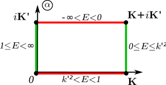
Figure 1: The sides of the rectangle are mapped by (2.4) onto the indicated energy intervals. The vertical (horizontal) sides shown in green (red) correspond to the two allowed (forbidden) bands. Vertices $\alpha={\rm{\bf K}}+i{\rm{\bf K}}^{\prime}$, ${\rm{\bf K}}$ and $0$ are mapped, respectively, into the edges $E=0$, $k^{\prime}{}^{2}$, and $1$ of the valence, $0\leq E\leq k^{\prime 2}$, and conduction, $1\leq E<\infty$, bands, which are described by periodic, $\mathrm{dn}\,x$ ($E=0$), and antiperiodic, $\mathrm{cn}\,x$ ($E=k^{\prime 2}$) and $\mathrm{sn}\,x$ ($E=1$), functions. Vertex $i{\rm{\bf K}}^{\prime}$ as a limit point on a horizontal (vertical) side corresponds to $E=-\infty$ ($E=+\infty$).

We have, particularly,

$$E({\rm{\bf K}}+i\beta)=k^{\prime}{}^{2}{\mathrm{cn}^{2}(\beta|k^{\prime})}{\mathrm{nd}^{2}(\beta|k^{\prime})}\,,\qquad 0\leq\beta\leq{\rm{\bf K}}^{\prime}\,,\quad k^{\prime}{}^{2}\geq E({\rm{\bf K}}+i\beta)\geq 0\,,$$ (2.5)

$$E(i\beta)={\mathrm{dn}^{2}(\beta|k^{\prime})}{\mathrm{nc}^{2}(\beta|k^{\prime})}=k^{\prime}{}^{2}+{k^{2}}{\mathrm{nc}^{2}(\beta|k^{\prime})}\,,\qquad 0\leq\beta<{\rm{\bf K}}^{\prime}\,,\quad 1\leq E(i\beta)<\infty\,.$$ (2.6)

For (2.5) and (2.6), eigenfunctions in (2.2) are bounded on a real line, that corresponds to the two allowed (valence and conduction) bands in the spectrum. In contrast, for $\alpha=\beta$ and $\alpha=\beta+i{\rm{\bf K}}^{\prime}$, $\beta\in(0,{\rm{\bf K}})$, a real part of ${\rm Z}(\alpha)$ is nonzero, and eigenfunctions (2.3) are not bounded for $|x|\rightarrow\infty$. This corresponds to the two forbidden zones, $-\infty<E<0$ and $k^{\prime}{}^{2}<E<1$.

Differentiation of (2.5) and (2.6) in $\beta$ gives a relation

$$\frac{dE}{d\beta}=2\eta(E)\sqrt{P(E)}\,,\qquad P(E)=E(E-k^{\prime}{}^{2})(E-1)\,.$$ (2.7)

The third order polynomial $P(E)$ takes positive values inside the allowed bands, and turns into zero at their edges. $\eta(E)$ takes values $-1$ and $+1$ in the valence and conduction bands, respectively.

Inside the two allowed bands, (2.3) are quasi-periodic Bloch wave functions,

$$\Psi^{\alpha}_{\pm}(x+2{\rm{\bf K}})=e^{\mp i2{\rm{\bf K}}\kappa(E)}\Psi^{\alpha}_{\pm}(x)\,,\qquad\kappa(E)=\frac{\pi}{2{\rm{\bf K}}}-i{\rm Z}(\alpha)\,,$$ (2.8)

where a first term in quasimomentum (crystal momentum) $\kappa(E)$ originates from the imparity of ${\rm H}$ function. In the valence, (2.5), and conduction, (2.6), bands its values are given by

$$\kappa(E({\rm{\bf K}}+i\beta))=\frac{\pi}{2{\rm{\bf K}}}-\left[{\rm Z}(\beta|k^{\prime})+\frac{\pi}{2{\rm{\bf K}}{\rm{\bf K}}^{\prime}}\beta-k^{\prime}{}^{2}\mathrm{cn}(\beta|k^{\prime})\mathrm{sn}(\beta|k^{\prime})\mathrm{nd}(\beta|k^{\prime})\right]\,,$$ (2.9)

$$\kappa(E(i\beta))=\frac{\pi}{2{\rm{\bf K}}}-\left[{\rm Z}(\beta|k^{\prime})+\frac{\pi}{2{\rm{\bf K}}{\rm{\bf K}}^{\prime}}\beta-\mathrm{dn}(\beta|k^{\prime})\mathrm{sn}(\beta|k^{\prime})\mathrm{nc}(\beta|k^{\prime})\right]\,.$$ (2.10)

With the help of (2.4) and (2.7) one finds a differential dispersion relation

$$\frac{d\kappa}{dE}=\eta(E)\,\frac{E-({\rm{\bf E}}/{\rm{\bf K}})}{2\sqrt{P(E)}}\,,$$ (2.11)

where ${\rm\bf{E}}$ is a complete elliptic integral of the second kind, see (B.1). Taking into account a relation $k^{\prime}{}^{2}<\frac{{\rm{\bf E}}}{{\rm{\bf K}}}<1$, see Appendix B, one finds that within the both allowed bands quasimomentum is increasing function of energy. It takes values $0$ and $\pi/2{\rm{\bf K}}$ at the edges $E=0$ and $E=k^{\prime}{}^{2}$ of the valence band, where Bloch-Floquet functions reduce to the periodic, $\mathrm{dn}\,x$, and antiperiodic, $\mathrm{cn}\,x$, functions in the real period $2{\rm{\bf K}}$ of the system. Within the conduction band, quasi-momentum increases from ${\pi}/{2{\rm{\bf K}}}$ to $+\infty$. At the lower edge $E=1$, two functions (2.3) reduce to the antiperiodic function $\mathrm{sn}\,x$. At all three edges of the allowed bands, derivative of quasimomentum in energy is $+\infty$. For large values of energy, $E\rightarrow+\infty$, we find that $\kappa(E)\approx\sqrt{E}$, i.e. Bloch functions (2.3) behave as the plane waves, $\Psi_{\pm}^{\alpha}(x+2{\rm{\bf K}})\approx e^{\mp i2{\bf{\rm K}}\sqrt{E}}\Psi_{\pm}^{\alpha}(x)$.

Second, linear independent solutions at the edges of the allowed bands $E_{i}=0,\,k^{\prime}{}^{2},\,1$ are $\Psi_{i}(x)=\psi_{i}(x)\mathcal{I}_{i}$, where $\mathcal{I}_{i}=\int dx/\psi_{i}^{2}(x)$, and $\psi_{i}=\mathrm{dn}\,x$, $\mathrm{cn}\,x$, $\mathrm{sn}\,x$, $i=1,2,3$. The integrals are expressed in terms of non-periodic incomplete elliptic integral of the second kind (B.2), $\mathcal{I}_{1}=\frac{1}{k^{\prime}{}^{2}}{\rm E}(x+{\rm{\bf K}})$, $\mathcal{I}_{2}=x-\frac{1}{k^{\prime}{}^{2}}{\rm E}(x+{\rm{\bf K}}+i{\rm{\bf K}}^{\prime})$, $\mathcal{I}_{3}=x-{\rm E}(x+i{\rm{\bf K}}^{\prime})$. $\Psi_{i}(x)$ are not bounded on $\mathbb{R}$ and correspond to non-physical states. These non-physical solutions follow also from general solutions (2.3). For instance, $\Psi_{3}(x)$ may be obtained as a limit of $(\Psi^{\alpha}_{+}(x)-\Psi^{\alpha}_{-}(x))/\alpha$ as $\alpha\rightarrow 0$. Eq. (2.3) provides a complete set of solutions for (2.2) as the second order differential equation. Notice also that Bloch states (2.3) within the allowed bands are related under complex conjugation as $(\Psi^{\alpha}_{+}(x))^{*}=\eta\Psi^{\alpha}_{-}(x)$, where $\eta$ is the same as in (2.7).

In conclusion of this section we note that the function $P(E)$ in Eqs. (2.7), (2.11) is a spectral polynomial. It will play a fundamental role in a nonlinear supersymmetry we will discuss below.

3 Self-isospectral Lamé system

Consider the lower in energy $E$ forbidden band by extending it with the edge value $E=0$ of the valence band. We introduce a notation $-2\tau+i{\rm{\bf K}}^{\prime}$ for the parameter $\alpha$ that corresponds to the extended interval $-\infty<E\leq 0$. By taking into account relations $\mathrm{dn}\,(-u)=\mathrm{dn}\,(u+2{\rm{\bf K}})=-\mathrm{dn}\,(u+2i{\rm{\bf K}}^{\prime})=\mathrm{dn}\,u$, it will be convenient do not restrict the values of $\tau$ to the interval $[-{\rm{\bf K}}/2,0)$, but assume that $\tau\in\mathbb{R}$, while keeping in mind that $E\rightarrow-\infty$ for $\tau\rightarrow n{\rm{\bf K}}$, $n\in\mathbb{Z}$. After a shift of the argument $x\rightarrow x+\tau$, the corresponding function $\Psi_{+}^{\alpha}$ from (2.3) with $\alpha=-2\tau+i{\rm{\bf K}}^{\prime}$ takes, up to an inessential multiplicative constant, the form

$$\frac{\Theta(x_{-})}{\Theta(x_{+})}\exp{\left[x\,{\rm z}(\tau)\right]}\equiv F(x;\tau)\,,$$ (3.1)

where we have introduced the notations $x_{+}=x+\tau$, $x_{-}=x-\tau$,

$${\rm z}(\tau)=-i\kappa(E(-2\tau+i{\rm{\bf K}}^{\prime}))=\varsigma(\tau)+{\rm Z}(2\tau)=\frac{1}{2}\frac{d}{d\tau}\ln(\Theta(2\tau)\,\mathrm{sn}\,2\tau)\,,$$ (3.2)

$$\varsigma(\tau)=\frac{1}{2}\frac{d}{d\tau}\ln\mathrm{sn}\,2\tau=\mathrm{ns}\,2\tau\,\mathrm{cn}\,2\tau\,\mathrm{dn}\,2\tau\,.$$ (3.3)

$F(x;\tau)$ is a quasi-periodic in $x$ and periodic in the $\tau$ function, $F(x+2{\rm{\bf K}};\tau)=\exp{\big{(}2{\rm{\bf K}}{\rm z}(\tau)\big{)}}F(x;\tau),$ $F(x;\tau+2{\rm{\bf K}})=F(x;\tau).$ It is a regular function of $\tau$, save for $\tau=n{\rm{\bf K}}$, $n\in\mathbb{Z}$, [which correspond to the poles $\alpha=2n{\rm{\bf K}}+i{\rm{\bf K}}^{\prime}$ of $\mathrm{dn}\,\alpha$ in (2.4)], where $F(x;\tau)$ with $x\neq 0$ undergoes infinite jumps from $0$ to $+\infty$. Since ${\rm z}({\rm{\bf K}}/2)=0$, function (3.1) reduces at $\tau={\rm{\bf K}}/2$ (up to an inessential multiplicative constant) to a periodic in the $x$ function $\mathrm{dn}\,(x+\frac{1}{2}{\rm{\bf K}})$ which describes a physical state with energy $E=0$ at the lower edge of the valence band of the system $H(x+\frac{1}{2}{\rm{\bf K}})$. $F(x;\tau)$ is a nodeless function that obeys the relations $F(x;-\tau)=F(-x;\tau)=1/F(x;\tau)$ and

$$\left[H(x_{+})+\varepsilon(\tau)\right]F(x;\tau)=0\,,\quad{\rm where}\quad\varepsilon(\tau)=-E(-2\tau+i{\rm{\bf K}}^{\prime})=\mathrm{cn}^{2}\,2\tau\,\mathrm{ns}^{2}\,2\tau\,.$$ (3.4)

Define a first order differential operator

$$\mathcal{D}(x;\tau)=F(x;\tau)\,\frac{d}{dx}\,\frac{1}{F(x;\tau)}=\frac{d}{dx}-\Delta(x;\tau)\,,\qquad\mathcal{D}^{\dagger}(x;\tau)=-\mathcal{D}(x;-\tau)\,,$$ (3.5)

where

$$\Delta(x;\tau)=\frac{F^{\prime}(x;\tau)}{F(x;\tau)}\,.$$ (3.6)

Operator (3.5) annihilates function (3.1), $\mathcal{D}(x;\tau)F(x;\tau)=0$, and we find that

$$\mathcal{D}^{\dagger}(x;\tau)\mathcal{D}(x;\tau)=H(x_{+})+\varepsilon(\tau)\,,\qquad\mathcal{D}(x;\tau)\mathcal{D}^{\dagger}(x;\tau)=H(x_{-})+\varepsilon(\tau)\,.$$ (3.7)

By virtue of $\varepsilon(\frac{1}{2}{\rm{\bf K}})=0$, a non-shifted Lamé Hamiltonian operator (2.1) factorizes then as $H(x)=\mathcal{D}\left(x+\frac{1}{2}{\rm{\bf K}};\frac{1}{2}{\rm{\bf K}}\right)\mathcal{D}^{\dagger}\left(x+\frac{1}{2}{\rm{\bf K}};\frac{1}{2}{\rm{\bf K}}\right)$. The alternative product produces a shifted in the half-period ${\rm{\bf K}}$ system, $H(x+{\rm{\bf K}})=\mathcal{D}^{\dagger}\left(x+\frac{{\rm{\bf K}}}{2};\frac{1}{2}{\rm{\bf K}}\right)\mathcal{D}\left(x+\frac{1}{2}{\rm{\bf K}};\frac{1}{2}{\rm{\bf K}}\right)\,.$ It is this factorization of a pair of Lamé Hamiltonians $H(x)$ and $H(x+{\rm{\bf K}})$ that underlies a usual supersymmetric structure studied in [28] in the light of a phenomenon of self-isospectrality.

Notice that while $F(x_{-};\tau)$ is, up to a multiplicative constant, a non-physical eigenfunction $\Psi^{-2\tau+iK^{\prime}}_{+}(x)$ of $H(x)$ of energy $-\varepsilon(\tau)$, function $F(x_{+};-\tau)=1/F(x_{+};\tau)$ coincides, up to a multiplicative constant, with another eigenfunction $\Psi^{-2\tau+iK^{\prime}}_{-}(x)$ of $H(x)$ with the same eigenvalue.

According to (3.7), the mutually shifted Hamiltonians $H(x+\tau)$ and $H(x-\tau)$ form a supersymmetric, self-isospectral periodic one-gap Lamé system

$$\mathcal{H}={\rm diag}\,(H(x_{+}),H(x_{-})),$$ (3.8)

see Fig. 2, for which $\Delta(x;\tau)$ plays the role of the superpotential that obeys the Ricatti equations

$$\Delta^{2}(x;\tau)\pm\Delta^{\prime}(x;\tau)=2k^{2}\mathrm{sn}^{2}(x\pm\tau)-k^{2}+\varepsilon(\tau)\,.$$ (3.9)

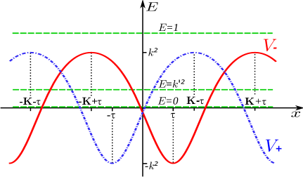
Figure 2: The self-isospectral potentials $V_{\pm}=2k^{2}\mathrm{sn}(x_{\pm})-k^{2}$ are shown together with the edges of the valence ($0\leq E\leq k^{\prime}{}^{2}$) and conduction ($1\leq E<\infty$) bands. $V_{\pm}$ have maxima at $x=\mp\tau+(2n+1){\rm{\bf K}}$ and minima at $x=\mp\tau+2n{\rm{\bf K}}$. Here $k^{2}=0.75$, ${\rm{\bf K}}=2.16$, and $\tau=0.8$.

Indeed, from factorizations (3.7) it follows that the $\mathcal{D}(x;\tau)$ and $\mathcal{D}^{\dagger}(x;\tau)$ intertwine the Hamiltonians $H(x_{+})$ and $H(x_{-})$,

$$\mathcal{D}(x;\tau)H(x_{+})=H(x_{-})\mathcal{D}(x;\tau)\,,\qquad\mathcal{D}^{\dagger}(x;\tau)H(x_{-})=H(x_{+})\mathcal{D}^{\dagger}(x;\tau)\,,$$ (3.10)

and interchange the eigenstates of the superpartner systems,

$$\mathcal{D}(x;\tau)\Psi^{\alpha}_{\pm}(x_{+})=\mathcal{F}^{\mathcal{D}}_{\pm}(\alpha,\tau)\,\Psi^{\alpha}_{\pm}(x_{-})\,,\quad\mathcal{D}^{\dagger}(x;\tau)\Psi^{\alpha}_{\pm}(x_{-})=-\mathcal{F}^{\mathcal{D}}_{\pm}(\alpha,-\tau)\,\Psi^{\alpha}_{\pm}(x_{+})\,.$$ (3.11)

The second relation in (3.11) follows from the first one via a substitution $\tau\rightarrow-\tau$. A complex amplitude, $\mathcal{F}^{\mathcal{D}}_{\pm}(\alpha,\tau)=e^{\pm i\varphi^{\mathcal{D}}(\alpha,\tau)}\mathcal{M}^{\mathcal{D}}(\alpha,\tau)$, is given by

$$\mathcal{F}^{\mathcal{D}}_{\pm}(\alpha,\tau)=-\exp\left[\mp 2i\left(\kappa(\alpha)-\frac{\pi}{2{\rm{\bf K}}}\right)\tau\right]\mathrm{ns}\,2\tau\,\frac{\Theta(2\tau\pm\alpha)\,\Theta(0)}{\Theta(2\tau)\Theta(\alpha)}\,.$$ (3.12)

It satisfies $\left(\mathcal{F}^{\mathcal{D}}_{\pm}(\alpha,\tau)\right)^{*}=\mathcal{F}^{\mathcal{D}}_{\mp}(\alpha,\tau)=-\mathcal{F}^{\mathcal{D}}_{\pm}(\alpha,-\tau).$ Its modulus may be presented in a form $\mathcal{M}^{\mathcal{D}}(\alpha,\tau)=\sqrt{E(\alpha)+\varepsilon(\tau)}\,,$ where $E(\alpha)$ for the valence and conduction bands is given by Eqs. (2.5) and (2.6). This agrees with Eq. (3.7). Notice that the modulus is an even in $\tau$ function, $\mathcal{M}^{\mathcal{D}}(\alpha,\tau)=\mathcal{M}^{\mathcal{D}}(\alpha,-\tau)$, which is nonzero except for the lower edge states of the valence band ($E=0$) in the case $\tau=(\frac{1}{2}+n){\rm{\bf K}}$. A phase is well defined for $\mathcal{M}^{\mathcal{D}}\neq 0$, and satisfies a relation

$$e^{i\varphi^{\mathcal{D}}(\alpha,-\tau)}=-e^{-i\varphi^{\mathcal{D}}\,(\alpha,\tau)}\,.$$ (3.13)

It can be presented in a form

$$e^{i\varphi^{\mathcal{D}}(\alpha,\tau)}=-{\rm sign}\,(\mathrm{ns}\,2\tau)\exp\left[-2i\left(\kappa(\alpha)-\frac{\pi}{2{\rm{\bf K}}}\right)\tau+i\varphi_{\Theta}(\alpha,\tau)\right],$$ (3.14)

where ${\rm sign}\,(.)$ is a sign function, and $\varphi_{\Theta}(\alpha,\tau)$ is a phase of $\Theta(2\tau+\alpha)$, $\varphi_{\Theta}(\alpha,\tau)={\rm Im}\left(\int_{0}^{2\tau+\alpha}Z(u)\,du\right),$ see Eq. (B.9). Particularly, for the edge states ($i=1,2,3$), Eq. (3.12) gives $\mathcal{D}(x;\tau)\psi_{i}(x_{+})=\mathcal{F}^{\mathcal{D}}_{i}(\tau)\psi_{i}(x_{-})$, $\mathcal{D}^{\dagger}(x;\tau)\psi_{i}(x_{-})=\mathcal{F}^{\mathcal{D}}_{i}(\tau)\psi_{i}(x_{+})$, where

$$\psi_{i}(x)=\mathrm{dn}\,x\,,\,\,\mathrm{cn}\,x\,,\,\,\mathrm{sn}\,x\,,\quad\mathcal{F}^{\mathcal{D}}_{i}(\tau)=-\mathrm{cn}\,2\,\tau\,\mathrm{ns}\,2\tau\,,\,\,-\mathrm{dn}\,2\,\tau\,\mathrm{ns}\,2\tau\,,\,\,-\mathrm{ns}\,2\tau\,,$$ (3.15)

and so,

$$\mathcal{M}^{\mathcal{D}}_{i}(\tau)=\sqrt{\varepsilon(\tau)}\,,\,\,\sqrt{k^{\prime}{}^{2}+\varepsilon(\tau)}\,,\,\,\sqrt{1+\varepsilon(\tau)}\,,$$ (3.16)

and $e^{i\varphi_{i}^{\mathcal{D}}(\tau)}=-{\rm sign}\,(\mathrm{cn}\,2\tau\,\mathrm{ns}\,2\tau)$, $-{\rm sign}\,(\mathrm{ns}\,2\tau),$ $-{\rm sign}\,(\mathrm{ns}\,2\tau).$

As a consequence of intertwining relations (3.10), first order matrix operators

$$S_{1}=\left(\begin{array}[]{cc}0&\mathcal{D}^{\dagger}(x;\tau)\\ \mathcal{D}(x;\tau)&0\\ \end{array}\right),\qquad S_{2}=i\sigma_{3}S_{1}\,,$$ (3.17)

are the integrals of motion for system (3.8). Integrals (3.17) correspond here (up to a unitary transformation of sigma matrices) to the first order operators $\hat{G}_{a}$ in section 1. Operator $\Gamma=\sigma_{3}$ is a trivial integral for (3.8), $[\Gamma,\mathcal{H}]=0$, that anticommutes with $S_{a}$, $a=1,2$, $\{\Gamma,S_{a}\}=0$, and classifies them as supercharges. Bosonic, $\mathcal{H}$, and fermionic, $S_{a}$, operators satisfy then the $N=2$ supersymmetry algebra,

$$\{S_{a},S_{b}\}=2\delta_{ab}(\mathcal{H}+\varepsilon(\tau))\,,\qquad[\mathcal{H},S_{a}]=0\,.$$ (3.18)

In correspondence with (3.11) and (3.13), the eigenstates of the supercharge $S_{1}$ are

$$S_{1}\Psi^{\alpha}_{\pm,S_{1},\epsilon}=\epsilon\mathcal{M}^{\mathcal{D}}(\alpha,\tau)\Psi^{\alpha}_{\pm,S_{1},\epsilon}\,,\quad\Psi^{\alpha}_{\pm,S_{1},\epsilon}=\left(\begin{array}[]{c}\Psi^{\alpha}_{\pm}(x_{+})\\ \epsilon e^{\pm i\varphi^{\mathcal{D}}(\alpha,\tau)}\Psi^{\alpha}_{\pm}(x_{-})\\ \end{array}\right),\quad\epsilon=\pm 1\,.$$ (3.19)

Since $\varepsilon(\tau)>0$ for $\tau\neq(\frac{1}{2}+n){\rm{\bf K}}$, $n\in\mathbb{Z}$, the first-order supersymmetry (3.18)  is dynamically broken in general case. It is unbroken however for $\tau=(n+\frac{1}{2}){\rm{\bf K}}$ by virtue of $\varepsilon((\frac{1}{2}+n){\rm{\bf K}})=0$. For these values of the shift parameter, the supercharges $S_{a}$ annihilate the ground states $\mathrm{dn}\,(x+(n+\frac{1}{2}){\rm{\bf K}})$ and $\mathrm{dn}\,(x-(n+\frac{1}{2}){\rm{\bf K}})$ of the super-partner systems $H(x+(n+\frac{1}{2}){\rm{\bf K}})$ and $H(x-(n+\frac{1}{2}){\rm{\bf K}})$. Notice that with variation of the shift parameter $\tau\neq n{\rm{\bf K}}$, which simultaneously governs the scale of the supersymmetry breaking $\varepsilon(\tau)$, the spectrum of the second order system (3.8) does not change. Each of its two super-partners has the same spectrum as a non-shifted Lamé system (2.1) does. Therefore, each energy level inside the valence, $0<E<k^{\prime}{}^{2}$, and conduction, $1<E<\infty$, bands is fourth-fold degenerate in accordance with the existence of the two Bloch states, $\Psi^{\alpha}_{\pm}(x_{+})$ and $\Psi^{\alpha}_{\pm}(x_{-})$, of the form (2.3) for each subsystem, see Eq. (3.19). We have a two-fold degeneration at the edges $E=0$, $E=k^{\prime}{}^{2}$ and $E=1$ of the valence and conduction bands in the spectrum of the supersymmetric system $\mathcal{H}$. Bosonic, $\Psi^{(+)}$, and fermionic, $\Psi^{(-)}$, states are defined as eigenstates of the grading operator $\Gamma=\sigma_{3}$, $\Gamma\Psi^{(\pm)}=\pm\Psi^{(\pm)}$, and have the general form $\Psi^{(+)}=(\Psi(x_{+}),0)^{T}$ and $\Psi^{(-)}=(0,\Psi(x_{-}))^{T}$, where $T$ means a transposition. In summary, we see that in both the broken and unbroken cases, the Witten index, which characterizes the difference between the number of bosonic and fermionic zero modes, is the same and equals zero.

For $\tau\neq(\frac{1}{2}+n){\rm{\bf K}}$ (when $\varepsilon(\tau)\neq 0$) supersymmetric relations (3.18) look differently from a usual form of superalgebra in supersymmetric quantum mechanics. A simple redefinition of the matrix Hamiltonian (3.8), $\mathcal{H}\rightarrow\tilde{\mathcal{H}}=\mathcal{H}+\varepsilon(\tau)$, will correct the form of superalgebraic relations, but will not change the conclusions on a broken (for $\tau\neq(\frac{1}{2}+n){\rm{\bf K}}$) form of the supersymmetric structure that we have analyzed. We shall return to this point in the discussion of the peculiar supersymmetry of the first order Bogoliubov-de Gennes system in section 7.

The described degeneracy of the energy levels in both, broken and unbroken, cases is unusual for $N=2$ supersymmetry. We will show that additional nontrivial integrals of motion may be associated with this peculiarity of the self-isospectral supersymmetric system (3.8). To identify such integrals, in the next section we investigate the function $\Delta(x;\tau)$ in greater detail.

4 Superpotential

Being the logarithmic derivative of $F(x;\tau)$, see Eq. (3.6), the superpotential $\Delta(x;\tau)$ may be written with the help of (B.11), (B.14) in terms of Jacobi’s ${\rm Z}$, or $\Theta$ and ${\rm H}$ functions,

$$\Delta(x;\tau)={\rm z}(\tau)+{\rm Z}(x_{-})-{\rm Z}(x_{+})=\frac{1}{2}\frac{\partial}{\partial\tau}\ln\left(\frac{{\rm H}(2\tau)}{\Theta^{2}(x_{-})\Theta^{2}(x_{+})}\right)\,.$$ (4.1)

The addition formula (B.6) for the ${\rm Z}$ function gives another, equivalent representation

$$\Delta(x;\tau)=\varsigma(\tau)+k^{2}\mathrm{sn}\,2\tau\,\mathrm{sn}\,(x_{-})\,\mathrm{sn}\,(x_{+})\,.$$ (4.2)

Functions ${\rm z}(\tau)$ and $\varsigma(\tau)$ are defined in (3.2), (3.3). Yet another useful representation for the superpotential may be derived from (4.2),

$$\Delta(x;\tau)=\frac{\mathrm{sn}\,x_{-}\mathrm{cn}\,x_{-}\mathrm{dn}\,x_{-}+\mathrm{sn}\,x_{+}\mathrm{cn}\,x_{+}\mathrm{dn}\,x_{+}}{\mathrm{sn}^{2}x_{+}-\mathrm{sn}^{2}x_{-}}\,.$$ (4.3)

Having in mind relations (3.10), (3.7) and (3.9), in what follows we treat $x$ as a variable and $\tau$ as a shift parameter. $\Delta(x;\tau)$ is an elliptic function in both its arguments with the same periods $2{\rm{\bf K}}$ and $2i{\rm{\bf K}}^{\prime}$. It is an even in $x$ and odd in the $\tau$ function with respect to the points $0,K$ (modulo periods), $\Delta(-x;\tau)=\Delta(x;\tau)$, $\Delta({\rm{\bf K}}-x;\tau)=\Delta({\rm{\bf K}}+x;\tau)$, $\Delta(x;-\tau)=-\Delta(x;\tau)$, $\Delta(x;{\rm{\bf K}}-\tau)=-\Delta(x;{\rm{\bf K}}+\tau)$. It also obeys a relation $\Delta(x+{\rm{\bf K}};\tau+{\rm{\bf K}})=\Delta(x-{\rm{\bf K}};\tau+{\rm{\bf K}})=\Delta(x;\tau)$. In $\tau=0,{\rm{\bf K}}$ the function undergoes infinite jumps.

Being the elliptic function in $x$, $\Delta(x;\tau)$ obeys a nonlinear differential equation

$${\Delta^{\prime}}^{2}=\Delta^{4}+2\delta_{2}(\tau)\Delta^{2}+\delta_{1}(\tau)\Delta+\delta_{0}(\tau)\,,$$ (4.4)

where $\delta_{2}(\tau)=1+k^{2}-3\mathrm{ns}^{2}\,2\tau$, $\delta_{1}(\tau)=8\mathrm{ns}^{3}\,2\tau\,\mathrm{cn}\,2\tau\,\mathrm{dn}\,2\tau$, and $\delta_{0}(\tau)=-3\mathrm{ns}^{4}\,2\tau+2(1+k^{2})\mathrm{ns}^{2}\,2\tau+k^{\prime}{}^{4}$. As a consequence of (4.4), it also satisfies the nonlinear higher order differential equations

$$\Delta^{\prime\prime}=2\Delta^{3}+2\delta_{2}(\tau)\Delta+\frac{1}{2}\delta_{1}(\tau)\,,\qquad\Delta^{\prime\prime\prime}=2\Delta^{\prime}\left(3\Delta^{2}+\delta_{2}(\tau)\right)\,.$$ (4.5)

Making use of (4.1), one finds the relation

$$\Delta(x+\tau+\lambda;\lambda)-\Delta(x+\lambda;\tau+\lambda)+\Delta(x;\tau)=g(\tau,\lambda)\,.$$ (4.6)

Function $g(\tau,\lambda)=\varsigma(\tau)+\varsigma(\lambda)-\varsigma(\tau+\lambda)+k^{2}\mathrm{sn}\,2\tau\,\mathrm{sn}\,2\lambda\,\mathrm{sn}\,2(\tau+\lambda)$ has symmetry properties $g(\tau,\lambda)=g(\lambda,\tau)=g(\tau,-\lambda-\tau)=-g(-\tau,-\lambda)$, and may be written as

$$g(\tau,\lambda)=\mathrm{ns}\,2\tau\,\mathrm{ns}\,2\lambda\,\mathrm{ns}\,2(\tau+\lambda)[1-\mathrm{cn}\,2\tau\,\mathrm{cn}\,2\lambda\,\mathrm{cn}\,2(\tau+\lambda)].$$ (4.7)

For a particular case $\lambda={\rm{\bf K}}/2$, to be important for non-periodic limit,

$$g\left(\tau,\frac{1}{2}{\rm{\bf K}}\right)=\mathcal{C}(\tau)\,,\qquad\mathcal{C}(\tau)=\mathrm{ns}\,2\tau\,\mathrm{nc}\,2\tau\,\mathrm{dn}\,2\tau\,.$$ (4.8)

Notice that $g(\tau,\lambda)$ takes nonzero values for all real values of its arguments . Equation (4.6) is a kind of addition formula for elliptic function $\Delta(x;\tau)$. Differentiating (4.6) in $x$ and using Ricatti equations (3.9), we obtain a relation

$$\Delta^{\prime}(x+\tau+\lambda;\lambda)-\Delta(x+\lambda;\tau+\lambda)\Delta(x+\tau+\lambda;\lambda)=$$

$$-\frac{1}{2}\left(\Delta^{2}(x;\tau)+\Delta^{\prime}(x;\tau)+\delta_{2}(\tau)\right)-g(\tau,\lambda)\Delta(x;\tau)+G(\tau,\lambda)\,,$$ (4.9)

where $G(\tau,\lambda)=\frac{1}{2}\left[1+k^{2}+g^{2}(\tau,\lambda)-\mathrm{ns}^{2}\,2\tau\,-\mathrm{ns}^{2}\,2\lambda-\mathrm{ns}^{2}\,2(\tau+\lambda)\right]\equiv 0$.

In conclusion of this section we note that functions $\delta_{a}(\tau)$, $a=0,1,2$, can be given a physical sense by expressing them in terms of the band edges energies and of $\varepsilon(\tau)$ : $\delta_{2}(\tau)=-(\tilde{E}_{1}^{2}+\tilde{E}_{2}^{2}+\tilde{E}_{3}^{2}),$ $\delta_{1}(\tau)=-2\frac{d\tilde{E}_{1}}{d\tau},$ $\delta_{0}(\tau)=-\delta_{2}(\tau)-2(\tilde{E}_{1}\tilde{E}_{2}+\tilde{E}_{1}\tilde{E}_{3}+\tilde{E}_{2}\tilde{E}_{3}),$ where $\tilde{E}_{i}(\tau)=E_{i}+\varepsilon(\tau)$, $E_{1}=0$, $E_{2}=k^{\prime}{}^{2}$ and $E_{3}=1$. Particularly, $\delta_{1}$ measures a velocity with which a scale of supersymmetry breaking changes as a function of the shift parameter. Notice also that the first equation in (4.5) has a form of a modified Ginzburg-Landau equation, see [43], which corresponds here to a gap equation for the real condensate field in the kink-antikink crystalline phase in the Gross-Neveu model with a bare mass term, see [6, 8]. At $\tau=(\frac{1}{2}+n){\rm{\bf K}}$ we have $\delta_{1}=0$, and superpotential $\Delta(x)$ satisfies the nonlinear Schrodinger equation, the lowest nontrivial member of the modified Korteweg-de Vries hierarchy [44]. This homogenisation of the second order nonlinear differential equation can be associated with restoration of the discrete chiral symmetry in (1.2) at $m_{0}=0$.

5 Higher order integrals and nonlinear superalgebra

Now we are in a position to identify higher order local intertwining operators and integrals of motion for the system $\mathcal{H}$. First, we find the second order intertwining operators. Changing $\tau\rightarrow-\lambda$ and shifting the argument $x\rightarrow x+\tau+\lambda$ in the first relation from (3.10), we obtain

$$\mathcal{D}(x+\tau+\lambda;-\lambda)H(x+\tau)=H(x+\tau+2\lambda)\mathcal{D}(x+\tau+\lambda;-\lambda).$$ (5.1)

Multiplying (5.1) by $\mathcal{D}(x+\lambda;\tau+\lambda)$ from the left, and using once again (3.10) on the right hand side, we obtain an intertwining relation

$$\mathcal{B}(x;\tau,\lambda)H(x_{+})=H(x_{-})\mathcal{B}(x;\tau,\lambda)\,.$$ (5.2)

It is generated by the second order differential operator

$$\mathcal{B}(x;\tau,\lambda)=\mathcal{D}(x+\lambda;\tau+\lambda)\mathcal{D}^{\dagger}(x+\tau+\lambda;\lambda)\,,$$ (5.3)

which is defined for $\lambda\,,\tau+\lambda\neq n{\rm{\bf K}}$. For adjoint operator we have $\mathcal{B}^{\dagger}(x;\tau,\lambda)H(x-\tau)=H(x+\tau)\mathcal{B}^{\dagger}(x;\tau,\lambda)$. In accordance with (5.1), the second order intertwining operator (5.3) shifts the Hamiltonian’s argument first for $2\lambda$ and then for $-2(\tau+\lambda)$. Equivalent representation of the operator (5.3) is

$$\mathcal{B}(x;\tau,\lambda)=-\mathcal{Y}(x;\tau)-g(\tau,\lambda)\mathcal{D}(x;\tau)\,,$$ (5.4)

$$\mathcal{Y}(x;\tau)=\frac{d^{2}}{dx^{2}}-\Delta(x;\tau)\frac{d}{dx}-\frac{1}{2}\left(\Delta^{2}(x;\tau)+\Delta^{\prime}(x;\tau)+\delta_{2}(\tau)\right)\,,\qquad\mathcal{Y}^{\dagger}(x;\tau)=\mathcal{Y}(x;-\tau)\,.$$ (5.5)

We have used here Eq. (4.6). So, the dependence of $\mathcal{B}(x;\tau,\lambda)$ on $\lambda$ is localized only in the $x$-independent multiplier $g(\tau,\lambda)$, see Eq. (4.7).

From Eqs. (5.3) and (3.10) it follows that at $\tau=0$ the second order intertwining operators $\mathcal{B}(x;\tau,\lambda)$ and $\mathcal{B}^{\dagger}(x;\tau,\lambda)$ reduce, up to an additive term $\varepsilon(\lambda)$, to the isospectral superpartner Hamiltonians, $\mathcal{B}(x;0,\lambda)=H(x)+\varepsilon(\lambda)$,  $\mathcal{B}^{\dagger}(x;0,\lambda)=H(x+2\lambda)+\varepsilon(\lambda).$

Forgetting for the moment on the $\tau=0$ case, from the viewpoint of intertwining relation (5.2), one could conclude that the parameter $\lambda$ has a “gauge-like”, non-observable nature. Such a conclusion, however, is not correct. We will return to this point later.

Since $g(\tau,\lambda)$ is nonzero for real $\tau$ and $\lambda$, operator $\mathcal{Y}(x;\tau)$, unlike $\mathcal{B}(x;\tau,\lambda)$, is not factorizable in terms of our first order intertwining operators (with real shift parameters) . Nevertheless, it is the second order intertwining operator as well as $\mathcal{B}(x;\tau,\lambda)$. It can be presented as a linear combination of the second and first order intertwining operators, $\mathcal{Y}(x;\tau)=-\mathcal{B}(x;\tau,\lambda)-g(\tau,\lambda)\mathcal{D}(x;\tau)$, and also may be used together with the first order operator $\mathcal{D}(x;\tau)$ to characterize the system. At the end of this section we shall discuss the peculiarities associated with such an alternative.

Having in mind a non-periodic limit we discuss later, it is convenient to fix $\lambda={\rm{\bf K}}/2$, and introduce a notation $\mathcal{A}(x;\tau)=\mathcal{B}\left(x;\tau,\frac{1}{2}{\rm{\bf K}}\right)$, i.e.

$$\mathcal{A}(x;\tau)=\mathcal{D}\left(x+\frac{1}{2}{\rm{\bf K}};\tau+\frac{1}{2}{\rm{\bf K}}\right)\mathcal{D}^{\dagger}\left(x+\tau+\frac{1}{2}{\rm{\bf K}};\frac{1}{2}{\rm{\bf K}}\right)=-\mathcal{Y}(x;\tau)-\mathcal{C}(\tau)\mathcal{D}(x;\tau)\,,$$ (5.6)

where $\mathcal{C}(\tau)$ is defined in Eq. (4.8). Employing the properties of $\mathcal{Y}(x;\tau)$ and $\mathcal{D}(x;\tau)$ under hermitian conjugation, from (5.6) one finds $\mathcal{A}^{\dagger}(x;\tau)=\mathcal{A}(x;-\tau)$, and then a representation alternative to (5.6) is obtained, $\mathcal{A}(x;\tau)=\mathcal{D}(x-\tau+\frac{1}{2}{\rm{\bf K}};\frac{1}{2}{\rm{\bf K}})\mathcal{D}^{\dagger}(x+\frac{1}{2}{\rm{\bf K}};-\tau+\frac{1}{2}{\rm{\bf K}})$. Unlike the operators $\mathcal{D}(x;\tau)$ and $\mathcal{Y}(x;\tau)$, the $\mathcal{A}(x;\tau)$ is well defined at $\tau=0$ and reduces just to a non-shifted Hamiltonian, $\mathcal{A}(x;0)=\mathcal{A}^{\dagger}(x;0)=H(x)$. Notice, however, that unlike $\mathcal{D}(x;\tau)$, it is not defined for $\tau=(\frac{1}{2}+n){\rm{\bf K}}$.

Second order intertwining operator of the most general form (5.3) may be presented in terms of the intertwining operators $\mathcal{A}(x;\tau)$ and $\mathcal{D}(x;\tau)$, $\mathcal{B}(x;\tau,\lambda)=\mathcal{A}(x;\tau)+\big{(}C(\tau)-g(\tau,\lambda)\big{)}\mathcal{D}(x;\tau).$

Because of Eq. (5.2), the self-isospectral system possesses (for $\tau\neq(\frac{1}{2}+n){\rm{\bf K}}$) the second order integrals

$$Q_{1}=\left(\begin{array}[]{cc}0&\mathcal{A}^{\dagger}(x;\tau)\\ \mathcal{A}(x;\tau)&0\\ \end{array}\right),\qquad Q_{2}=i\sigma_{3}Q_{1}\,$$ (5.7)

to be nontrivial for $\tau\neq n{\rm{\bf K}}$ and independent from the first order integrals (3.17).

With some algebraic manipulations, we find

$$\mathcal{A}^{\dagger}(x;\tau)\mathcal{A}(x;\tau)=H(x_{+})\left[H(x_{+})+\varrho(\tau)\right]\,,\quad{\rm where}\quad\varrho(\tau)=k^{\prime}{}^{2}\mathrm{sn}^{2}\,2\tau\,\mathrm{nc}^{2}\,2\tau\,.$$ (5.8)

A similar relation is obtained from (5.8) by a simple change $\tau\rightarrow-\tau$, $\mathcal{A}(x;\tau)\mathcal{A}^{\dagger}(x;\tau)=H(x_{-})\left[H(x_{-})+\varrho(\tau)\right].$ cf. relations in (3.7) for the first order intertwining operators.

The intertwining second order operator $\mathcal{A}(x;\tau)$ annihilates the lower energy state $\mathrm{dn}\,(x+\tau)$ of the system $H(x+\tau)$. Another state annihilated by it is

$$f(x,\tau)=\mathrm{dn}\,(x+\tau)\int^{x}\frac{F(u+\frac{1}{2}{\rm{\bf K}};\tau+\frac{1}{2}{\rm{\bf K}})}{\mathrm{dn}\,(u+\tau)}du\,,$$ (5.9)

and we have $f(x+2K,\tau)=\exp\left[2{\rm{\bf K}}{\rm z}(\tau+\frac{1}{2}{\rm{\bf K}})\right]\,f(x,\tau)$. Function (5.9) for $\tau\neq 0$ is unbounded and describes therefore a non-physical eigenstate of $H(x+\tau)$ from the lower forbidden band with energy $E=-\varrho(\tau)<0$, see Eq. (5.8). At $\tau=0$, function (5.9) reduces to ${\rm E}(x+{\rm{\bf K}})\,\mathrm{dn}\,x$ that corresponds to a nonphysical state of $H(x)$ of zero eigenvalue.

Like the first order operator $\mathcal{D}(x;\tau)$, $\mathcal{A}(x;\tau)$ transforms the eigenstates of $H(x+\tau)$ into those of $H(x-\tau)$,

$$\mathcal{A}(x;\tau)\Psi^{\alpha}_{\pm}(x_{+})=\mathcal{F}^{\mathcal{A}}_{\pm}(\alpha,\tau)\,\Psi^{\alpha}_{\pm}(x_{-})\,,$$ (5.10)

where

$$\mathcal{F}^{\mathcal{A}}_{\pm}(\alpha,\tau)=e^{\pm i\varphi^{\mathcal{A}}(\alpha,\tau)}\mathcal{M}^{\mathcal{A}}(\alpha,\tau)\,,\quad\mathcal{M}^{\mathcal{A}}(\alpha,\tau)=\sqrt{E(\alpha)(E(\alpha)+\varrho(\tau))}\,.$$ (5.11)

The modulus and the phase of the complex amplitude $\mathcal{F}^{\mathcal{A}}_{\pm}(\alpha,\tau)$ are expressed in terms of those for the first order intertwining operator by employing Eqs. (5.1), (5.6) and (3.11),

$$\mathcal{M}^{\mathcal{A}}(\alpha,\tau)=\mathcal{M}^{\mathcal{D}}\left(\alpha,\tau+\frac{1}{2}{\rm{\bf K}}\right)\mathcal{M}^{\mathcal{D}}\left(\alpha,\frac{1}{2}{\rm{\bf K}}\right)\,,\quad\varphi^{\mathcal{A}}(\alpha,\tau)=\varphi^{\mathcal{D}}(\alpha,\tau+\frac{1}{2}{\rm{\bf K}})-\varphi^{\mathcal{D}}(\alpha,\frac{1}{2}{\rm{\bf K}})\,.\qquad$$ (5.12)

A phase $\varphi^{\mathcal{A}}(\alpha,\tau)\in\mathbb{R}$ has, unlike (3.13), a property $e^{i\varphi^{\mathcal{A}}(\alpha,-\tau)}=e^{-i\varphi^{\mathcal{A}}(\alpha,\tau)}$ due to a relation $\mathcal{A}^{\dagger}(x;\tau)=\mathcal{A}(x;-\tau)$ to be different in sign from that for the first order intertwining operator, $\mathcal{D}^{\dagger}(x;\tau)=-\mathcal{D}(x;-\tau)$. For the edge band states, particularly, we have $\mathcal{A}(x;\tau)\psi_{i}(x_{+})=\mathcal{F}^{\mathcal{A}}_{i}(\tau)\psi_{i}(x_{-})$, $\mathcal{A}^{\dagger}(x;\tau)\psi_{i}(x_{-})=\mathcal{F}^{\mathcal{A}}_{i}(\tau)\psi_{i}(x_{+}),$ where $\mathcal{F}^{\mathcal{A}}_{i}(\tau)=0\,,\,\,k^{\prime}{}^{2}\mathrm{nc}\,2\tau\,,\,\,\mathrm{dn}\,2\tau\,\mathrm{nc}\,2\tau$, $i=1,2,3$, cf. (3.15). The eigenstates of the integral $Q_{1}$, see (5.7), have a form similar to that for $S_{1}$,

$$Q_{1}\Psi^{\alpha}_{\pm,Q_{1},\epsilon}=\epsilon\mathcal{M}^{\mathcal{A}}(\alpha,\tau)\Psi^{\alpha}_{\pm,Q_{1},\epsilon}\,,\quad\Psi^{\alpha}_{\pm,Q_{1},\epsilon}=\left(\begin{array}[]{c}\Psi^{\alpha}_{\pm}(x_{+})\\ \epsilon e^{\pm i\varphi^{\mathcal{A}}(\alpha,\tau)}\Psi^{\alpha}_{\pm}(x_{-})\\ \end{array}\right),\quad\epsilon=\pm 1\,.$$ (5.13)

Two relations are valid for the first and second order intertwining operators,

$$\mathcal{D}^{\dagger}(x;\tau)\mathcal{A}(x;\tau)=\mathcal{P}(x_{+})-\mathcal{C}(\tau)H(x_{+})\,,\quad\mathcal{D}(x;\tau)\mathcal{A}^{\dagger}(x;\tau)=-\mathcal{P}(x_{-})-\mathcal{C}(\tau)H(x_{-})\,.$$ (5.14)

Here $\mathcal{P}(x_{+})=\mathcal{P}(x+\tau)$ is an anti-hermitian third order differential operator

$$\mathcal{P}(x_{+}) = \frac{d^{3}}{dx^{3}}-\frac{3}{2}\left(\Delta^{2}+\Delta^{\prime}+\frac{1}{3}\delta_{2}(\tau)\right)\frac{d}{dx}-\frac{3}{4}\left(\Delta^{2}+\Delta^{\prime}\right)^{\prime}\quad$$ (5.15)

$$= \frac{d^{3}}{dx^{3}}+\left(1+k^{2}-3k^{2}\mathrm{sn}^{2}x_{+}\right)\frac{d}{dx}-3k^{2}\mathrm{sn}\,x_{+}\,\mathrm{cn}\,x_{+}\,\mathrm{dn}\,x_{+}\,.\quad$$

Notice that like the Lamé Hamiltonian, the operator (5.15) is well defined for any value of the shift parameter $\tau$. Two related equalities may be obtained from (5.14) by hermitian conjugation.

Making use of intertwining relations (3.10), (5.2), we find that $H(x+\tau)$ commutes with $\mathcal{D}^{\dagger}(x;\tau)\mathcal{A}(x;\tau)$, and, therefore, $\mathcal{P}(x+\tau)$ is an integral for the subsystem $H(x+\tau)$. For self-isospectral supersymmetric system $\mathcal{H}$ we have then two further, third order hermitian integrals

$$L_{1}=-i\,{\rm diag}\,\left(\mathcal{P}(x_{+}),\mathcal{P}(x_{-})\right),\qquad L_{2}=\sigma_{3}L_{1}\,.$$ (5.16)

Operator $\mathcal{P}(x)$ is a Lax operator for the periodic one-gap Lamé system $H(x)$, see [38, 39].

The following relations that involve the operator $\mathcal{P}(x_{+})$ are valid,

$$\mathcal{D}(x;\tau)\mathcal{P}(x+\tau)=\mathcal{A}(x;\tau)\left[H(x_{+})+\varepsilon(\tau)\right]+\mathcal{C}(\tau)\mathcal{D}(x;\tau)H(x_{+})\,,$$ (5.17)

$$\mathcal{A}(x;\tau)\mathcal{P}(x_{+})=-\mathcal{D}(x;\tau)H(x_{+})\left[H(x_{+})+\varrho(\tau)\right]-\mathcal{C}(\tau)\mathcal{A}(x;\tau)H(x_{+})\,,$$ (5.18)

$$-\mathcal{P}^{2}(x_{+})=P(H(x_{+}))\,,\qquad P(H)=H(H-k^{\prime}{}^{2})(H-1)\,.$$ (5.19)

The third order polynomial $P(H)$ is the same spectral polynomial of the Lamé system that arose before in (2.7) and in differential dispersion relation (2.11) : it turns into zero when acts on the edge states with energies $E_{i}=0,k^{\prime}{}^{2},1$. Since the third order differential operator $\mathcal{P}(x_{+})$ is an integral of motion for $H(x_{+})$, relation (5.19) means that the edge states $\mathrm{dn}\,x_{+}$, $\mathrm{cn}\,x_{+}$ and $\mathrm{sn}\,x_{+}$ form its kernel [39]. The spectral polynomial is a semi-positive definite operator, while $\mathcal{P}(x)$ is an anti-hermitian operator. Its action on physical Bloch states (2.3) should reduce therefore to $\pm i\sqrt{P(E(\alpha))}$. The phase cannot change abruptly within the allowed bands. To fix correctly the sign, one can consider a limit $k\rightarrow 0$, in which Lamé system (2.1) reduces to a free particle, an integral $\mathcal{P}(x)$ reduces to a third order operator $d^{3}/dx^{3}+d/dx$, forbidden zone $k^{\prime}{}^{2}<E<1$ disappears, Bloch states transform into the plane wave states, whereas the edge states $\mathrm{dn}\,x$, $\mathrm{cn}\,x$ and $\mathrm{sn}\,x$ reduce, respectively, to $1$, $\cos x$ and $\sin x$ with energies $E=0,\,1$ and $1$. Summarizing all this, one finds that the operator (5.15) acts on the physical Bloch states (2.3) as follows,

$$\mathcal{P}(x)\Psi^{\alpha}_{\pm}(x)=\mp i\eta(E)\sqrt{P(E(\alpha))}\,\Psi^{\alpha}_{\pm}(x)\,,$$ (5.20)

where, as in (2.7) and (2.11), $\eta(E)=-1$ for valence and $+1$ for conduction bands . Relation (5.20) means, particularly, that the Lax operator is not reduced just to a square root from the spectral polynomial since Hamiltonian does not distinguish index $\pm$. This is a true, nontrivial integral of motion that is related with the Hamiltonian $H$ by polynomial equation (5.19) . Eq. (5.19) corresponds to a non-degenerate spectral elliptic curve of genus one associated with a one-gap periodic Lamé system [35].

Let us discuss now the superalgebra generated by the zero, $\sigma_{3}$, first, $S_{a}$, second, $Q_{a}$, and third, $L_{a}$, order integrals of motion of the self-isospectral system $\mathcal{H}$. The operator $\Gamma=\sigma_{3}$ commutes with $L_{a}$ and anti-commutes with $Q_{a}$, and so, classifies them, respectively, as bosonic and fermionic operators. Using the displayed relations for the operators $\mathcal{D}$, $\mathcal{A}$ and $\mathcal{P}$ as well as those obtained from them by a hermitian conjugation and by a change $\tau\rightarrow-\tau$, Eq. (3.18) is extended by the anti-commutation relations of the integrals $S_{a}$ with $Q_{a}$, and the commutation relations of $S_{a}$ and $Q_{a}$ with $L_{a}$. We arrive as a result at the following superalgebra for the self-isospectral system (3.8) with $\mathbb{Z}_{2}$ grading operator $\Gamma=\sigma_{3}$,

$$\{S_{a},S_{a}\}=2\delta_{ab}\big{(}\mathcal{H}+\varepsilon(\tau)\big{)},\qquad\{Q_{a},Q_{b}\}=2\delta_{ab}\mathcal{H}\big{(}\mathcal{H}+\varrho(\tau)\big{)},$$ (5.21)

$$\{S_{a},Q_{b}\}=2\left(-\delta_{ab}\,\mathcal{C}(\tau)\mathcal{H}+\epsilon_{ab}\,L_{1}\right),$$ (5.22)

$$[L_{1},S_{a}]=[L_{1},Q_{a}]=[L_{1},L_{2}]=0\,,\qquad[L_{2},S_{a}]=2i\big{(}S_{a}\mathcal{C}(\tau)\mathcal{H}+Q_{a}(\mathcal{H}+\varepsilon(\tau))\big{)}\,,$$ (5.23)

$$[L_{2},Q_{a}]=-2i\big{(}S_{a}\mathcal{H}(\mathcal{H}+\varrho(\tau))+Q_{a}\mathcal{C}(\tau)\mathcal{H}\big{)}\,,$$ (5.24)

$$[\sigma_{3},S_{a}]=-2i\epsilon_{ab}S_{b},\quad[\sigma_{3},Q_{a}]=-2i\epsilon_{ab}Q_{b},\quad[\sigma_{3},L_{a}]=0,$$ (5.25)

$$[\mathcal{H},\sigma_{3}]=[\mathcal{H},S_{a}]=[\mathcal{H},Q_{a}]=[\mathcal{H},L_{a}]=0\,.$$ (5.26)

We have here a nonlinear superalgebra, in which $L_{1}$ (that is a Lax operator for $\mathcal{H}$) plays a role of the bosonic central charge, and $\sigma_{3}$ is treated as one of its even generators in correspondence with $\mathbb{Z}_{2}$ grading relations $[\sigma_{3},\sigma_{3}]=[\sigma_{3},\mathcal{H}]=[\sigma_{3},L_{a}]=0$ and $\{\sigma_{3},S_{a}\}=\{\sigma_{3},Q_{a}\}=0$.

Since $L_{1}$ commutes with $S_{a}$ and $Q_{a}$, the eigenstates (3.19) and (5.13) of $S_{1}$ and $Q_{1}$ are simultaneously the eigenstates of $L_{1}$,

$$L_{1}\Psi^{\alpha}_{\pm,\Lambda,\epsilon}=\mp\eta\sqrt{P(\alpha)}\,\Psi^{\alpha}_{\pm,\Lambda,\epsilon}\,,$$ (5.27)

where $\Lambda=S_{1}$ or $Q_{1}$, $\eta$ is the same as in (2.11) and (5.20), and $P(\alpha)=P(E(\alpha))$. Note that unlike $S_{1}$ and $Q_{1}$, $L_{1}$ distinguishes the index $\pm$.

In correspondence with the discussion related to (5.9), the $Q_{a}$, $a=1,2$, annihilate the two ground states of zero energy, $\mathrm{dn}\,(x+\tau)$ and $\mathrm{dn}\,(x-\tau)$, while other two states from their kernel are non-physical. These supercharges are not defined, however, for $\tau=(\frac{1}{2}+n){\rm{\bf K}}$, which are the only values of the shift parameter when the $N=2$ supersymmetry associated with the first order supercharges $S_{a}$ is not broken. Therefore, when the first and the second order supercharges are simultaneously defined [for $\tau\neq(\frac{1}{2}+n){\rm{\bf K}},\,n{\rm{\bf K}}$], the supersymmetry generated together by $S_{a}$ and $Q_{a}$ is partially broken.

One could construct, instead, the second order supercharges, $Q^{\mathcal{Y}}_{a}$, on the basis of the intertwining operators $\mathcal{Y}(x;\tau)$ and $\mathcal{Y}^{\dagger}(x;\tau)$. According to (5.6), they are related to $Q_{a}$ as

$$Q^{\mathcal{Y}}_{a}=-Q_{a}-\mathcal{C}(\tau)S_{a}\,.$$ (5.28)

The corresponding super-algebra with $Q_{a}$ substituted for $Q^{\mathcal{Y}}_{a}$ will have then a form similar to that we have discussed, with the change of some of the corresponding (anti)-commutators for

$$\{Q^{\mathcal{Y}}_{a},Q^{\mathcal{Y}}_{b}\}=2\delta_{ab}\big{(}\mathcal{H}(\mathcal{H}+\varrho(\tau)-\mathcal{C}^{2}(\tau))+\varepsilon(\tau)\mathcal{C}^{2}(\tau)\big{)},$$ (5.29)

$$\{S_{a},Q^{\mathcal{Y}}_{b}\}=-2\big{(}\delta_{ab}\,\sigma_{3}\,\mathcal{C}(\tau)\varepsilon(\tau)+\epsilon_{ab}\,L_{1}\big{)}\,,$$ (5.30)

$$[L_{2},S_{a}]=-2i\big{(}S_{a}\mathcal{C}(\tau)\varepsilon(\tau)+Q^{\mathcal{Y}}_{a}(\mathcal{H}+\varepsilon(\tau))\big{)}\,,$$ (5.31)

$$[L_{2},Q^{\mathcal{Y}}_{a}]=2i\big{(}S_{a}\mathcal{H}(\mathcal{H}+\varrho(\tau)+\varepsilon(\tau)\mathcal{C}(\tau)-\mathcal{C}^{2}(\tau))+Q^{\mathcal{Y}}_{a}\varepsilon(\tau)\mathcal{C}(\tau)\big{)}\,.$$ (5.32)

The second order supercharges $Q^{\mathcal{Y}}_{a}$, like $S_{a}$, are well defined at $\tau=(\frac{1}{2}+n){\rm{\bf K}}$ but not defined for $\tau=n{\rm{\bf K}}$. Analyzing the roots of the polynomial in the right hand side of (5.29), one finds that the kernels of $Q^{\mathcal{Y}}_{a}$, $a=1,2$, for $\tau\neq(\frac{1}{2}+n){\rm{\bf K}}$ are formed by non-physical states. In the exceptional case $\tau=(\frac{1}{2}+n){\rm{\bf K}}$, for which the supercharges $Q_{a}$ are not defined, the polynomial in (5.29) reduces to the second order polynomial

$$P_{Q^{\mathcal{Y}}}(\mathcal{H})=(\mathcal{H}-k^{\prime}{}^{2})(\mathcal{H}-1)\,.$$ (5.33)

In correspondence with this, the zero modes of the operators $\mathcal{Y}(x;\frac{1}{2}{\rm{\bf K}})$ and $\mathcal{Y}^{\dagger}(x;\frac{1}{2}{\rm{\bf K}})=\mathcal{Y}(x;-\frac{1}{2}{\rm{\bf K}})$ are, respectively, the physical edge states $\mathrm{cn}\,(x+\frac{1}{2}{\rm{\bf K}})$, $\mathrm{sn}\,(x+\frac{1}{2}{\rm{\bf K}})$ and $\mathrm{cn}\,(x-\frac{1}{2}{\rm{\bf K}})$, $\mathrm{sn}\,(x-\frac{1}{2}{\rm{\bf K}})$. This property reflects a peculiarity of the case $\tau=(\frac{1}{2}+n){\rm{\bf K}}$ in another aspect. In accordance with footnote 5, function $g(\tau,\lambda)$ in (5.4) turns into zero at $\lambda=\frac{1}{2}({\rm{\bf K}}+i{\rm{\bf K}}^{\prime})$. The second order operator $\mathcal{Y}(x;\frac{1}{2}{\rm{\bf K}})$ factorizes then either as $\mathcal{Y}(x;\frac{1}{2}{\rm{\bf K}})=-\mathcal{D}(x+\frac{1}{2}({\rm{\bf K}}+i{\rm{\bf K}}^{\prime});{\rm{\bf K}}+\frac{1}{2}i{\rm{\bf K}}^{\prime})\mathcal{D}^{\dagger}(x+{\rm{\bf K}}+\frac{1}{2}i{\rm{\bf K}}^{\prime};\frac{1}{2}({\rm{\bf K}}+i{\rm{\bf K}}^{\prime}))$, or in alternative form obtained by the change of $i$ for $-i$. These two factorizations can be presented equivalently as

$$\mathcal{Y}(x;\frac{1}{2}{\rm{\bf K}})=\left(\mathrm{ns}\,(x-\frac{1}{2}{\rm{\bf K}})\frac{d}{dx}\mathrm{sn}\,(x-\frac{1}{2}{\rm{\bf K}})\right)\left(\mathrm{cn}\,(x+\frac{1}{2}{\rm{\bf K}})\frac{d}{dx}\mathrm{nc}\,(x+\frac{1}{2}{\rm{\bf K}})\right)\,,$$ (5.34)

$$\mathcal{Y}(x;\frac{1}{2}{\rm{\bf K}})=\left(\mathrm{nc}\,(x-\frac{1}{2}{\rm{\bf K}})\frac{d}{dx}\mathrm{cn}\,(x-\frac{1}{2}{\rm{\bf K}})\right)\left(\mathrm{sn}\,(x+\frac{1}{2}{\rm{\bf K}})\frac{d}{dx}\mathrm{ns}\,(x+\frac{1}{2}{\rm{\bf K}})\right)\,.$$ (5.35)

From here we see that the particular case of the half period shift of the super-partner systems is indeed exceptional. In this case not only the $N=2$ supersymmetry associated with the first order supercharges $S_{a}$ is unbroken (when zero modes of $S_{a}$ are the ground states that form a zero energy doublet), but all the other edge states of the energy doublets with $E=k^{\prime}{}^{2}$ and $E=1$ correspond to zero modes of the second order supercharges $Q^{\mathcal{Y}}_{a}$. Then the third order spectral polynomial $P(\mathcal{H})=\mathcal{H}(\mathcal{H}-k^{\prime}{}^{2})(\mathcal{H}-1)$ is just a product of the first and the second order polynomials which correspond to the squares of the first, $S_{a}$, and the second, $Q^{\mathcal{Y}}_{a}$, order supercharges. In this special case the (anti-)commutation relations (5.30), (5.31), (5.32) also simplify their form, $\{S_{a},Q^{\mathcal{Y}}_{b}\}=-2\epsilon_{ab}\,L_{1},$ $[L_{2},S_{a}]=-2iQ^{\mathcal{Y}}_{a}\mathcal{H},$ $[L_{2},Q^{\mathcal{Y}}_{a}]=2iS_{a}P_{Q^{\mathcal{Y}}}(\mathcal{H}).$ We also have

$$S_{a}Q^{\mathcal{Y}}_{a}=-Q^{\mathcal{Y}}_{a}S_{a}=-iL_{2}\,,\qquad S_{a}Q^{\mathcal{Y}}_{b}=Q^{\mathcal{Y}}_{b}S_{a}=-L_{1}\,,$$ (5.36)

where there is no summation in index $a$, and $b\neq a$. This is in conformity with the above mentioned factorization of the spectral polynomial. However, since $Q^{\mathcal{Y}}_{a}$ does not annihilate the ground states $\mathrm{dn}\,(x+\frac{1}{2}{\rm{\bf K}})$ and $\mathrm{dn}\,(x-\frac{1}{2}{\rm{\bf K}})$ (which are transformed mutually by the intertwining operators $\mathcal{Y}(x;\frac{1}{2}{\rm{\bf K}})$ and $\mathcal{Y}^{\dagger}(x;\frac{1}{2}{\rm{\bf K}})$), we conclude that nonlinear supersymmetry of the self-isospectral system also is partially broken at $\tau=(\frac{1}{2}+n){\rm{\bf K}}$ .

In the next section we will see that another peculiarity of our self-isospectral system is that the choice $\Gamma=\sigma_{3}$ is not unique for identification of the $\mathbb{Z}_{2}$ grading operator : it also admits other choices for $\Gamma$, which lead to different identifications of the integrals $\sigma_{3}$, $S_{a}$, $Q_{a}$ and $L_{a}$ as bosonic and fermionic operators. This results in the alternative forms for the superalgebra. Each of such alternative forms of the superalgebra makes, particularly, a nontrivial relation (5.19) to be ‘visible’ explicitly just in its structure, unlike the case with $\Gamma=\sigma_{3}$ that we have discussed. We also will identify the integrals of motion which detect the phases in the structure of the eigenstates of the operators $S_{a}$ and $Q_{a}$.

6 Nonlocal $\mathbb{Z}_{2}$ grading operators

Let us introduce the operators of reflection in $x$ and $\tau$, $\mathcal{R}x\mathcal{R}=-x$, $\mathcal{R}\tau\mathcal{R}=\tau$, $\mathcal{R}^{2}=1$, $\mathcal{T}\tau\mathcal{T}=-\tau$, $\mathcal{T}x\mathcal{T}=x$, $\mathcal{T}^{2}=1$. They intertwine the superpartner Hamiltonians, $\mathcal{R}H(x_{+})=H(x_{-})\mathcal{R}$, $\mathcal{T}H(x_{+})=H(x_{-})\mathcal{T}$, and we find that the self-isospectral supersymmetric system (3.8) possesses the hermitian integrals of motion

$$\mathcal{R}\sigma_{1},\quad\mathcal{T}\sigma_{1},\quad\mathcal{R}\sigma_{2},\quad\mathcal{T}\sigma_{2},\quad\mathcal{RT}\sigma_{3},\quad\mathcal{RT}\,.$$ (6.1)

Like for $\sigma_{3}$, a square of each of them equals 1. From relations

$$\mathcal{R}\mathcal{D}(x;\tau)=\mathcal{D}^{\dagger}(x;\tau)\mathcal{R}\,,\quad\mathcal{R}\mathcal{A}(x;\tau)=\mathcal{A}^{\dagger}(x;\tau)\mathcal{R}\,,\quad\mathcal{R}\mathcal{P}(x_{+})=-\mathcal{P}(x_{-})\mathcal{R}\,,$$ (6.2)

$$\mathcal{T}\mathcal{D}(x;\tau)=-\mathcal{D}^{\dagger}(x;\tau)\mathcal{T}\,,\quad\mathcal{T}\mathcal{A}(x;\tau)=\mathcal{A}^{\dagger}(x;\tau)\mathcal{T}\,,\quad\mathcal{T}\mathcal{P}(x_{+})=\mathcal{P}(x_{-})\mathcal{T}\,,$$ (6.3)

it follows that $\mathcal{R}$ and $\mathcal{T}$ intertwine also the operators of the same order within the pairs ($\mathcal{D}(x;\tau)$, $\mathcal{D}^{\dagger}(x;\tau)$), ($\mathcal{A}(x;\tau)$, $\mathcal{A}^{\dagger}(x;\tau)$), and ($\mathcal{P}(x_{+})$, $\mathcal{P}(x_{-})$). As a result, each of the nonlocal in $x$ or $\tau$, or in both of them, integrals of motion (6.1) either commutes or anti-commutes with each of the nontrivial local integrals $S_{a}$, $Q_{a}$ and $L_{a}$. Then each integral from (6.1) also may be chosen as the $\mathbb{Z}_{2}$ grading operator for the self-isospectral system (3.8). Corresponding $\mathbb{Z}_{2}$ parities together with those prescribed by a local integral $\sigma_{3}$ are shown in Table 1. $\mathbb{Z}_{2}$ parities of the second order integrals $Q^{\mathcal{Y}}_{a}$, defined in (5.28), are also displayed; the equality $\mathcal{C}(-\tau)=-\mathcal{C}(\tau)$ has to be employed in their computation. Notice that $Q^{\mathcal{Y}}_{a}$, $a=1,2$, always has the same $\mathbb{Z}_{2}$ parity as the $Q_{a}$ with the same value of the index $a$.

Table 1: $\mathbb{Z}_{2}$ parities of the local integrals.

$\Gamma$	$\sigma_{3}$	$S_{1}$	$S_{2}$	$Q_{1}$, $Q^{\mathcal{Y}}_{1}$	$Q_{2}$, $Q^{\mathcal{Y}}_{2}$	$L_{1}$	$L_{2}$
$\sigma_{3}$	$+$	$-$	$-$	$-$	$-$	$+$	$+$
$\mathcal{R}\sigma_{1}$	$-$	$+$	$-$	$+$	$-$	$-$	$+$
$\mathcal{T}\sigma_{1}$	$-$	$-$	$+$	$+$	$-$	$+$	$-$
$\mathcal{R}\sigma_{2}$	$-$	$-$	$+$	$-$	$+$	$-$	$+$
$\mathcal{T}\sigma_{2}$	$-$	$+$	$-$	$-$	$+$	$+$	$-$
$\mathcal{R}\mathcal{T}\sigma_{3}$	$+$	$+$	$+$	$-$	$-$	$-$	$-$
$\mathcal{R}\mathcal{T}$	$+$	$-$	$-$	$+$	$+$	$-$	$-$

A positive $\mathbb{Z}_{2}$ parity is assigned for the Hamiltonian $\mathcal{H}$ by any of the integrals (6.1). Then for any choice of the grading operator presented in Table 1, four of the eight local integrals $\sigma_{3}$, $\mathcal{H}$, $S_{a}$, $L_{a}$ and $Q_{a}$ or $Q^{\mathcal{Y}}_{a}$ are identified as bosonic generators, and four are identified as fermionic generators of the corresponding nonlinear superalgebra. The superalgebra may be found for each choice of $\Gamma$ from the set of integrals (6.1) by employing the quadratic products of the operators $\mathcal{D}$, $\mathcal{A}$ and $\mathcal{P}$ that have been discussed in the previous section. Alternatively, some of the (anti)-commutators may be obtained with the help of the already known (anti)-commutation relations and relations between the generators that involve $\sigma_{3}$. For instance, $[S_{1},Q_{1}]=i\sigma_{3}\{S_{1},Q_{2}\}$. As an example, we display the explicit form of the superalgebraic relations for the choice $\Gamma=\mathcal{RT}$,

$$\{S_{a},S_{b}\}=2\delta_{ab}\big{(}\mathcal{H}+\varepsilon(\tau)\big{)}\,,\quad\{S_{a},L_{1}\}=2\epsilon_{ab}\big{(}Q_{b}(\mathcal{H}+\varepsilon(\tau))+\mathcal{C}(\tau)S_{b}\mathcal{H}\big{)}\,,\quad\{S_{a},L_{2}\}=0\,,$$ (6.4)

$$\{L_{1},L_{1}\}=\{L_{2},L_{2}\}=2P(\mathcal{H}),\qquad\{L_{1},L_{2}\}=2\sigma_{3}P(\mathcal{H}),$$ (6.5)

$$[Q_{a},S_{b}]=2i\big{(}-\delta_{ab}L_{2}+\epsilon_{ab}\mathcal{C}(\tau)\sigma_{3}\mathcal{H}\big{)},\qquad[Q_{1},Q_{2}]=-2i\sigma_{3}\mathcal{H}\big{(}\mathcal{H}+\varrho(\tau)\big{)},$$ (6.6)

$$[Q_{a},L_{1}]=0,\qquad[Q_{a},L_{2}]=2i\big{(}\mathcal{C}(\tau)Q_{a}\mathcal{H}+S_{a}\mathcal{H}(\mathcal{H}+\varrho(\tau))\big{)},$$ (6.7)

which should be supplied by the commutation relations (5.25) and (5.26). $P(\mathcal{H})$ in (6.5) is the spectral polynomial, see (5.19).

A fundamental polynomial relation (5.19) between the Lax operator and the Hamiltonian, that underlies a very special, finite-gap nature of Lamé system , does not show up in the superalgebraic structure for a usual choice of the diagonal matrix $\sigma_{3}$ as the grading operator $\Gamma$, but is involved explicitly in the superalgebra in the form of the anticommutator of one or both generators $L_{a}$, $a=1,2$, when any of six non-local integrals (6.1) is identified as $\Gamma$.

Note that for $\Gamma=\mathcal{RT}$ as well as for any other choice of the grading operator that involves the operator $\mathcal{T}$, the constant $\mathcal{C}(\tau)$ anticommutes with the grading operator and should be treated as an odd generator of the superalgebra. As a result, the right hand side in the second anticommutator in (6.4) is an even operator, while the right hand side in the first (second) commutator in (6.6) (in (6.7)) is an odd operator as it should be.

By employing Eq. (5.28), one can rewrite superalgebraic relations (6.4), (6.6) and (6.7) in terms of the integrals $Q^{\mathcal{Y}}_{a}$, which, unlike $Q_{a}$, are defined for $\tau=(\frac{1}{2}+n){\rm{\bf K}}$. We do not display them here, but write down only a commutation relation

$$[S_{a},Q^{\mathcal{Y}}_{b}]=2i\big{(}\delta_{ab}L_{2}+\sigma_{3}\epsilon_{ab}\mathcal{C}(\tau)\varepsilon(\tau)\big{)}\,,$$ (6.8)

which we will need below. The form of such a superalgebra simplifies significantly at $\tau=(\frac{1}{2}+n){\rm{\bf K}}$ in correspondence with a special nature that the integrals $S_{a}$ and $Q_{a}^{\mathcal{Y}}$ acquire in the case. Particularly, one finds

$$\{S_{a},S_{b}\}=2\delta_{ab}\mathcal{H}\,,\qquad\{S_{a},L_{1}\}=-2\epsilon_{ab}Q^{\mathcal{Y}}_{b}\mathcal{H}\,,$$ (6.9)

$$[Q^{\mathcal{Y}}_{a},S_{b}]=2i\delta_{ab}L_{2}\,,\qquad[Q^{\mathcal{Y}}_{1},Q^{\mathcal{Y}}_{2}]=-2i\sigma_{3}P_{Q^{\mathcal{Y}}}(\mathcal{H})\,,\qquad[L_{2},Q^{\mathcal{Y}}_{a}]=2iS_{a}P_{Q^{\mathcal{Y}}}(\mathcal{H})\,.$$ (6.10)

All the integrals (6.1) including $\sigma_{3}$ but excluding $\mathcal{RT}$ may be related between themselves by unitary transformations, whose generators are constructed in terms of the grading operators themselves. For instance, $U\sigma_{3}U^{\dagger}=\mathcal{R}\sigma_{1}=\tilde{\sigma_{3}}$, $U=U^{\dagger}=U^{-1}=\frac{1}{\sqrt{2}}(\sigma_{3}+\mathcal{R}\sigma_{1}).$ Being constructed from the integrals of motion, such a transformation does not change the supersymmetric Hamiltonian $\mathcal{H}$. On the other hand, if we apply it to any nontrivial integral, the transformed operator still will be an integral. Particularly, its application to the integrals $S_{1}$ and $Q_{1}$ gives

$$\tilde{S}=i\mathcal{R}\sigma_{2}S_{1}={\rm diag}\,\left(\mathcal{RD}(x;\tau),-\mathcal{RD}^{\dagger}(x;\tau)\right),\quad\tilde{Q}=i\mathcal{R}\sigma_{2}Q_{1}={\rm diag}\,\left(\mathcal{RA}(x;\tau),-\mathcal{RA}^{\dagger}(x;\tau)\right).$$ (6.11)

These are nontrivial hermitian nonlocal integrals of motion for the self-isospectral system (3.8) . Eq. (6.11) has a sense of Foldy-Wouthuysen transformation that diagonalizes the supercharges $S_{1}$ and $Q_{1}$. The price we pay for this is a non-locality of the transformed operators.

Multiplication of (6.11) by the grading operators gives further nonlocal integrals, particularly, $\sigma_{3}\tilde{S}$ and $\sigma_{3}\tilde{Q}$. Since the both operators (6.11) are diagonal, the Lamé subsystem $H(x_{+})$ may be characterized, in addition to the Lax integral $\mathcal{P}(x_{+})$, by two nontrivial nonlocal integrals

$$\hat{S}=\mathcal{RD}(x;\tau)\,,\qquad\hat{Q}=\mathcal{RA}(x;\tau)\,.$$ (6.12)

In correspondence with relations $\mathcal{D}^{\dagger}(x;\tau)=-\mathcal{D}(x;-\tau)$ and $\mathcal{A}^{\dagger}(x;\tau)=\mathcal{A}(x;-\tau)$, another subsystem $H(x_{-})$ is characterized then by the integrals of the same form but with $\tau$ changed for $-\tau$. The operator $\hat{\Gamma}=\mathcal{RT}$ is an integral for the subsystem $H(x_{+})$ [as well as for subsystem $H(x_{-})$]. It can be identified as a $\mathbb{Z}_{2}$ grading operator that assigns definite $\mathbb{Z}_{2}$ parities for nontrivial integrals of the subsystem $H(x_{+})$. Namely, in correspondence with (6.2) and (6.3), the integrals $-i\mathcal{P}(x_{+})$ and $\hat{S}$ are fermionic operators with respect to such a grading, while $\hat{Q}$ should be treated as a bosonic operator. Multiplying fermionic integrals by $i\hat{\Gamma}$ and bosonic integral by $\hat{\Gamma}$, we obtain three more integrals for $H(x_{+})$. It is not difficult to calculate the corresponding superalgebra generated by these integrals. Let us note only that since the described supersymmetry may be revealed in the subsystem $H(x_{+})$ (or, in $H(x_{-})$), it may be treated as a bosonized supersymmetry, see [47, 37, 38].

Let us return to the question of degeneration in our self-isospectral system. This will allow us to observe some other interesting properties related to the nonlocal integrals (6.1). Let us take a pair of mutually commuting integrals $S_{1}$ and $L_{1}$. They can be simultaneously diagonalized, and for their common eigenstates we have $S_{1}\Psi^{\alpha}_{\pm,S_{1},\epsilon}=\epsilon\mathcal{M}^{\mathcal{D}}(\alpha,\tau)\Psi^{\alpha}_{\pm,S_{1},\epsilon}$ and $L_{1}\Psi^{\alpha}_{\pm,S_{1},\epsilon}=\mp\eta(\alpha)\sqrt{P(\alpha)}\,\Psi^{\alpha}_{\pm,S_{1},\epsilon}$, see Eqs. (3.19) and (5.27). We can distinguish all the four states by these relations for any value of the energy within the valence and conduction bands, and each two doublet states for the edges $E=0,k^{\prime}{}^{2},1$ of the allowed bands when $\tau\neq(\frac{1}{2}+n){\rm{\bf K}}$. However, in the case of $\tau=(\frac{1}{2}+n){\rm{\bf K}}$, the two ground states of zero energy are annihilated by the both operators $S_{1}$ and $L_{1}$, and cannot be distinguished by them. In this special case the operator $\sigma_{3}$ commutes with $S_{1}$ and $L_{1}$ on the subspace $E=0$, and may be used to distinguish the two ground states. It is necessary to remember, however, that $\sigma_{3}$ does not commute with $S_{1}$ on the subspaces of nonzero energy.

There is yet another possibility. According to Table 1, the local integrals $S_{1}$ and $L_{1}$ commute with the nonlocal integral $\mathcal{T}\sigma_{2}$. We find then

$$\mathcal{T}\sigma_{2}\Psi^{\alpha}_{\pm,S_{1},\epsilon}=i\epsilon e^{\mp i\varphi^{\mathcal{D}}(\alpha,\tau)}\Psi^{\alpha}_{\pm,S_{1},\epsilon}\,,$$ (6.13)

where we used relation (3.14). The operator $\mathcal{T}\sigma_{2}$ detects therefore the phase in the structure of the eigenstates of $S_{1}$. By comparing two supersymmetric systems with the shift parameters $\tau$ and $\tau+{\rm{\bf K}}$, and by taking into account the $2{\rm{\bf K}}$-periodicity of the $\Theta$ function in (3.12) and the $2{\rm{\bf K}}$-anti-periodicity of $\mathrm{sn}\,u$, we get from (3.14) that $e^{i\left(\varphi^{D}(\alpha,\tau+{\rm{\bf K}})-\varphi^{D}(\alpha,\tau)\right)}=e^{\frac{i}{{\rm{\bf K}}}\kappa(\alpha)\tau}$. Hence the integral $\mathcal{T}\sigma_{2}$ makes, particularly, the same job as a translation for the period operator (which is also a nonlocal integral for the system) : it allows us to determine an energy-dependent quasi-momentum. Finally, in the case of zero energy ($\alpha={\rm{\bf K}}+i{\rm{\bf K}}^{\prime}$), treating $\tau=(\frac{1}{2}+n){\rm{\bf K}}$ as a limit case, one can also distinguish two ground states in the supersymmetric doublet by means of (6.13).

Instead of $S_{1}$, $L_{1}$ and $\mathcal{T}\sigma_{2}$, we could choose the triplet $S_{2}$, $L_{1}$ and $\mathcal{T}\sigma_{1}$ of mutually commuting integrals, see Table 1. The states within the supermultiplets can be distinguished also by choosing the triplets of mutually commuting integrals ($Q_{1}$, $L_{1}$, $\mathcal{T}\sigma_{1}$), or ($Q_{2}$, $L_{1}$, $\mathcal{T}\sigma_{2}$). For the two latter cases, the doublet of the ground states is annihilated by $Q_{a}$ and $L_{1}$ for any value of the shift parameter $\tau$ (excluding the case $\tau=(\frac{1}{2}+n){\rm{\bf K}}$ when $Q_{a}$ are not defined), but the corresponding integrals $\mathcal{T}\sigma_{1}$ or $\mathcal{T}\sigma_{2}$ do here the necessary job of distinguishing the states as well.

The integrals $\mathcal{R}\sigma_{1}$ and $\mathcal{RT}\sigma_{3}$ act on the eigenstates of $S_{1}$, with which they also commute, as $\mathcal{R}\sigma_{1}\Psi^{\alpha}_{\pm,S_{1},\epsilon}(x,\tau)=-\epsilon e^{\pm i\varphi^{\mathcal{D}}(\alpha,\tau)}\Psi^{\alpha}_{\mp,S_{1},\epsilon}(x,\tau),$ $\mathcal{RT}\sigma_{3}\Psi^{\alpha}_{\pm,S_{1},\epsilon}(x,\tau)=-\Psi^{\alpha}_{\mp,S_{1},\epsilon}(x,\tau).$ These operators interchange the states with $+$ and $-$ indexes, and anti-commute with the integral $L_{1}$. The edge states, which do not carry such an index, are annihilated by $L_{1}$, so that there is no contradiction with the information presented in Table 1.

In conclusion of this section we note that the Witten index computed with the grading operator identified with any of the six nonlocal integrals (6.1) is the same as for a choice $\Gamma=\sigma_{3}$, i. e. $\Delta_{W}=0$.

7 Supersymmetry of the associated periodic BdG system

Till the moment we have discussed the self-isospectrality of the one-gap Lamé system with the second order Hamiltonian. Though we have shown that its supersymmetric structure is much more rich than a usual one, from the viewpoint of the physics of the GN model it is more natural to look at the revealed picture from another perspective.

Let us take one of the first order integrals $S_{a}$ of the self-isospectral Lamé system, say $S_{1}$, and consider it as a first order, Dirac Hamiltonian. In such a way we obtain an intimately related, but different physical system. Unlike the second order operator $\mathcal{H}$, the spectrum (3.19) of $S_{1}$ depends on $\tau$. We get a periodic Bogoliubov-de Gennes system with Hamiltonian $H_{BdG}=S_{1}$. The interpretation of the function $\Delta(x;\tau)$ changes in this case : this is a Dirac scalar potential in correspondence with a discussion from section 1. In dependence on a physical context, it takes a sense of an order parameter, a condensate, or a gap function.

The $\tau$-dependent spectrum of such a BdG system consists of four or three allowed bands located symmetrically with respect to the level $\mathcal{E}=0$, see Figure 3. Interpretation of the bands also changes and depends on the physical context. For $\tau\neq(\frac{1}{2}+n){\rm{\bf K}}$, the positive and negative ‘internal’ bands are separated by a nonzero gap $\Delta\mathcal{E}(\tau)=2\sqrt{\varepsilon(\tau)}=2|\mathrm{cn}\,2\tau\,\mathrm{ns}\,2\tau|$, which disappears at $\tau=(\frac{1}{2}+n){\rm{\bf K}}$. The total number of gaps in the spectrum is three in the case $\tau\neq(\frac{1}{2}+n){\rm{\bf K}}$, $\mathcal{E}\in(-\infty,\mathcal{E}_{3,-}]\,\cup\,[\mathcal{E}_{2,-},\mathcal{E}_{1,-}]\,\cup\,[\mathcal{E}_{1,+},\mathcal{E}_{2,+}]\,\cup\,[\mathcal{E}_{3,+},\infty)$, while for $\tau=(\frac{1}{2}+n){\rm{\bf K}}$ there are only two gaps, $\mathcal{E}\in(-\infty,\mathcal{E}_{3,-}]\,\cup\,[\mathcal{E}_{2,-},\mathcal{E}_{2,+}]\,\cup\,[\mathcal{E}_{3,+},\infty)$. According to (3.15), (3.16) and (3.19), the edges $\mathcal{E}_{i,\epsilon}$ of the internal ($i=1,2$) and external ($i=3$) allowed bands are

$$\mathcal{E}_{1,\epsilon}(\tau)=\epsilon\sqrt{\varepsilon(\tau)}\,,\qquad\mathcal{E}_{2,\epsilon}(\tau)=\epsilon\sqrt{k^{\prime}{}^{2}+\varepsilon(\tau)}\,,\qquad\mathcal{E}_{3,\epsilon}(\tau)=\epsilon\sqrt{1+\varepsilon(\tau)}\,,$$ (7.1)

where $\epsilon=\pm$, and the eigenstates have a form $\Psi_{i,\epsilon}(x,\tau)=\left(\psi_{i}(x_{+}),\epsilon e^{i\varphi^{\mathcal{D}}_{i}(\tau)}\psi_{i}(x_{-})\right)^{T},$ $S_{1}\Psi_{i,\epsilon}(x,\tau)=\mathcal{E}_{i,\epsilon}\Psi_{i,\epsilon}(x,\tau).$

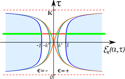
Figure 3: Spectrum of $H_{BdG}=S_{1}$ possesses symmetries $\mathcal{E}_{\epsilon}(\alpha,\tau)=\mathcal{E}_{\epsilon}(\alpha,-\tau)=\mathcal{E}_{\epsilon}(\alpha,\tau+{\rm{\bf K}})$, $\mathcal{E}_{\epsilon}(\alpha,\frac{1}{2}{\rm{\bf K}}+\tau)=\mathcal{E}_{\epsilon}(\alpha,\frac{1}{2}{\rm{\bf K}}-\tau)$, and $\mathcal{E}_{-}(\alpha,\tau)=-\mathcal{E}_{+}(\alpha,\tau)$. Horizontal line shows a spectrum for some value of $\tau$, $\frac{1}{2}{\rm{\bf K}}<\tau<{\rm{\bf K}}$. The allowed (forbidden) bands on it are presented by thick green (thin red) intervals, whose points are distinguished by the parameter $\alpha$, see Eq. (7.2). Curves indicate the edges of the allowed bands (7.1). The point $\mathcal{E}_{\epsilon}({\rm{\bf K}}+i{\rm{\bf K}}^{\prime},\frac{1}{2}{\rm{\bf K}})=0$ corresponds to a doubly degenerate energy level in the allowed band $[-k^{\prime},k^{\prime}]$, that is formed by the two merging at $\tau=\frac{1}{2}{\rm{\bf K}}$ internal allowed bands.

In the context of the physics of conducting polymers, for example, the internal bands are referred to as the lower, $[\mathcal{E}_{2,-},\mathcal{E}_{1,-}]$, and upper, $[\mathcal{E}_{1,+},\mathcal{E}_{2,+}]$, polaron bands; the upper external band, $[\mathcal{E}_{3,+},\infty)$, is called the conduction band; the lower external band, $(-\infty,\mathcal{E}_{3,-}]$, is referred to as the valence band [31]. In general case for eigenstates (3.19) we have

$$S_{1}\Psi^{\alpha}_{\pm,S_{1},\epsilon}(x,\tau)=\mathcal{E}_{\epsilon}(\alpha,\tau)\Psi^{\alpha}_{\pm,S_{1},\epsilon}(x,\tau)\,,\qquad\mathcal{E}_{\epsilon}(\alpha,\tau)=\epsilon\sqrt{E(\alpha)+\varepsilon(\tau)}\,,$$ (7.2)

where $E(\alpha)$ for internal and external bands is given by Eqs. (2.5) and (2.6).

Since $H_{BdG}=S_{1}$ does not distinguish index $\pm$ of the wave functions within the allowed bands, each corresponding energy level is doubly degenerate. Six edge states for $\tau\neq(\frac{1}{2}+n){\rm{\bf K}}$ are singlets. In the case $\tau=(\frac{1}{2}+n){\rm{\bf K}}$, four edge states with energies $\mathcal{E}=\pm k^{\prime}$ and $\pm 1$ are singlets. Zero energy states $\Psi_{1,\epsilon}$ form a doublet in this case, as it happens for any other energy level inside any allowed band.

The described degeneration in the spectrum of $S_{1}$ indicates that the BdG system might possess its own nonlinear supersymmetric structure. This is indeed the case. First of all, from Table 1 we see that there are three operators, $\mathcal{R}\sigma_{1}$, $\mathcal{T}\sigma_{2}$ and $\mathcal{RT}\sigma_{3}$, which commute with $S_{1}$, and square of each equals one. Hence, each of them may be chosen as a $\mathbb{Z}_{2}$ grading operator for the BdG system. There are three more, nontrivial local integrals of motion for $H_{BdG}$. One is the second order operator $\mathcal{H}$. This, however, is not interesting from the viewpoint of a supersymmetric structure since it is just a shifted square of $H_{BdG}=S_{1}$, $\mathcal{H}=S_{1}^{2}-\varepsilon(\tau)$. Then we have a third order integral $L_{1}\equiv\mathcal{L}_{1}$, that has been identified before as the Lax operator for the self-isospectral Lamé system $\mathcal{H}$. Finally, the fourth order operator $\mathcal{G}_{1}=S_{1}\mathcal{L}_{1}$ is also identified as a local integral of motion. Note that the both integrals $\mathcal{L}_{1}$ and $\mathcal{G}_{1}$ distinguish the states inside the allowed bands, which differ in index $\pm\,$. On distinguishing the states with $\mathcal{E}=0$ to be present in the spectrum if $\tau=(\frac{1}{2}+n){\rm{\bf K}}$, see a discussion at the end of the previous section. Further nontrivial, but nonlocal integrals may be obtained if we multiply local integrals by the operators $\mathcal{R}\sigma_{1}$, $\mathcal{T}\sigma_{2}$ and $\mathcal{RT}\sigma_{3}$. Then, as in the case of the self-isospectral Lamé system, different choices for the grading operator lead to distinct identifications of $\mathbb{Z}_{2}$ parities of the integrals.

For the sake of definiteness, let us choose $\Gamma=\mathcal{R}\sigma_{1}$, and assume first that $\tau\neq(\frac{1}{2}+n){\rm{\bf K}}$. Other two possibilities for the choice of $\Gamma$ may be considered in an analogous way. If, additionally, we restrict our analysis by the integrals that do not include in their structure a nonlocal in $\tau$ operator $\mathcal{T}$, we get two $\mathbb{Z}_{2}$-even (commuting with $\Gamma$) integrals in addition to $H_{BdG}=S_{1}$, namely, $\mathcal{R}\sigma_{1}$ and $\mathcal{R}\sigma_{1}S_{1}$. The four $\mathbb{Z}_{2}$-odd (anticommuting with $\Gamma$) integrals are $\mathcal{L}_{1}$, $\mathcal{G}_{1}$, $\mathcal{L}_{2}=i\mathcal{R}\sigma_{1}\mathcal{L}_{1}$ and $\mathcal{G}_{2}=i\mathcal{R}\sigma_{1}\mathcal{G}_{1}$. All these integrals are hermitian operators. It is interesting to note that a nonlocal integral $\mathcal{R}\sigma_{1}S_{1}$ is related to one of the diagonal nonlocal operators from (6.11), $\mathcal{R}\sigma_{1}S_{1}=\sigma_{3}\tilde{S}$. A nonlocal diagonal operator $\mathcal{G}_{2}$ also may be related to (6.11), $\mathcal{G}_{2}=\tilde{Q}S_{1}^{2}+\mathcal{C}(\tau)\tilde{S}(S_{1}^{2}-\varepsilon(\tau))$. Since, however, integrals $\mathcal{R}\sigma_{1}S_{1}$ and $\mathcal{G}_{a}$ are just the integrals $\mathcal{R}\sigma_{1}$ and $\mathcal{L}_{a}$ multiplied by the BdG Hamiltonian $S_{1}$, we can forget them as well as $\mathcal{H}$. We obtain then nontrivial (anti)commutation relations of the nonlinear BdG superalgebra,

$$[\mathcal{R}\sigma_{1},\mathcal{L}_{a}]=-2i\epsilon_{ab}\mathcal{L}_{b}\,,\qquad\{\mathcal{L}_{a},\mathcal{L}_{b}\}=2\delta_{ab}\hat{P}(S_{1},\tau)\,.$$ (7.3)

Here, in correspondence with Eqs. (5.19), (5.21) and (6.5), $\hat{P}(S_{1},\tau)$ is the six order spectral polynomial of the BdG system,

$$\hat{P}(S_{1},\tau)=(S_{1}^{2}-\varepsilon(\tau))(S_{1}^{2}-\varepsilon(\tau)-k^{\prime}{}^{2})(S_{1}^{2}-\varepsilon(\tau)-1)\,,$$ (7.4)

whose six roots correspond to the energy levels (7.1).

Superalgebra (7.3) has a structure similar to that of a hidden, bosonized supersymmetry [47] of the unextended Lamé system (2.1), which was revealed in [38]. There, the role of the grading operator is played by a reflection operator $\mathcal{R}$, the matrix integrals $\mathcal{L}_{a}$ are substituted by the Lax operator $-i\mathcal{P}(x)$, see Eq. (5.15), and by $\mathcal{R}\mathcal{P}(x)$. The six order polynomial $\hat{P}(S_{1},\tau)$ of the BdG Hamiltonian $S_{1}$ is changed there for a third order spectral polynomial $P(H)$, see Eq. (5.19).

We have seen that the structure of the BdG spectrum changes significantly at $\tau=(\frac{1}{2}+n){\rm{\bf K}}$. Essential changes happen also in the superalgebraic structure. Indeed, from (6.8) it follows that $[S_{1},Q^{\mathcal{Y}}_{2}]=2i\sigma_{3}\epsilon_{ab}\mathcal{C}(\tau)\varepsilon(\tau)$, i. e. in a generic case $Q^{\mathcal{Y}}_{2}$ does not commute with $H_{BdG}$. In contrary, for $\tau=(\frac{1}{2}+n){\rm{\bf K}}$ this is an additional nontrivial, second order integral of motion of the BdG system. This integral, like the third order integral $L_{1}$, also distinguishes the states marked by the index $\pm$ inside the allowed bands, $Q^{\mathcal{Y}}_{2}\Psi^{\alpha}_{\pm,S_{1},\epsilon}=\pm\eta\sqrt{P_{Q^{\mathcal{Y}}}(E(\alpha))}\,\Psi^{\alpha}_{\pm,S_{1},\epsilon}$, where $\eta$ is the same as in (2.11) and (5.20), i.e. $\eta=-1$ for $0\leq E\leq k^{\prime}{}^{2}$ and $\eta=+1$ for $E\geq 1$, while $P_{Q^{\mathcal{Y}}}(E)$ is a polynomial that appeared earlier in (5.33), i. e. $P_{Q^{\mathcal{Y}}}(E)=(E-k^{\prime}{}^{2})(E-1)$. In this case, $L_{1}$ is not independent integral for the BdG system anymore since here $L_{1}=-S_{1}Q^{\mathcal{Y}}_{2}$ in correspondence with (5.36). Integral $Q^{\mathcal{Y}}_{2}$ anticommutes with $\mathcal{R}\sigma_{1}$ and $\mathcal{RT}\sigma_{3}$. Let us choose, again, $\Gamma=\mathcal{R}\sigma_{1}$, and denote $\mathcal{Q}_{1}=Q^{\mathcal{Y}}_{2}$ and $\mathcal{Q}_{2}=i\Gamma\mathcal{Q}_{1}$. Instead of (7.3), we get a nonlinear superalgebra of the order four,

$$[\mathcal{R}\sigma_{1},\mathcal{Q}_{a}]=-2i\epsilon_{ab}\mathcal{Q}_{b}\,,\qquad\{\mathcal{Q}_{a},\mathcal{Q}_{b}\}=2\delta_{ab}\hat{P}_{\mathcal{Q}}(S_{1})\,,$$ (7.5)

where $\hat{P}_{\mathcal{Q}}(S_{1})=(S_{1}^{2}-k^{\prime}{}^{2})(S_{1}^{2}-1)$.

It is interesting to see what happens with the Witten index in the described unusual supersymmetry of the BdG system with the first order Hamiltonian. One can construct the eigenstates of the grading operator $\Gamma=\mathcal{R}\sigma_{1}$,

$$\Gamma\Psi^{(\epsilon)}(x;\alpha,\tau)=-\epsilon\Psi^{(\epsilon)}(x;\alpha,\tau)\,,\quad\Psi^{(\epsilon)}(x;\alpha,\tau)\equiv\Psi^{\alpha}_{+,S_{1},\epsilon}(x,\tau)+e^{i\varphi^{\mathcal{D}}(\alpha,\tau)}\Psi^{\alpha}_{-,S_{1},\epsilon}(x,\tau)\,.$$ (7.6)

For any energy value inside any allowed band (including $\mathcal{E}=0$ in the case of $\tau=(\frac{1}{2}+n){\rm{\bf K}}$), we have two states with opposite eigenvalues of $\Gamma$, and these contribute zero into the Witten index $\Delta_{W}={\rm Tr}\,\Gamma$, where trace is taken over all the eigenstates of the grading operator $\Gamma$. On the other hand, the edge states $\Psi_{i,\epsilon}(x,\tau)$ are singlets. They are also the eigenstates of $\Gamma$. The eigenstates of opposite energy signs have opposite eigenvalues, $+1$ and $-1$, of the grading operator. As a result, we conclude that the Witten index $\Delta_{W}$ in such a supersymmetric system equals zero for any value of $\tau$ [i.e., for $\tau\neq(\frac{1}{2}+n){\rm{\bf K}}$ when there are no zero energy states in the spectrum, and for $\tau=(\frac{1}{2}+n){\rm{\bf K}}$ when the spectrum contains a doublet of zero energy states], like this happens in the self-isospectral Lamé system with the second order supersymmetric Hamiltonian. The same result $\Delta_{W}=0$ is obtained for the choices $\Gamma=\mathcal{T}\sigma_{2}$ and $\Gamma=\mathcal{RT}\sigma_{3}$.

Finally, it is worth to notice that in accordance with the structure of superalgebra (7.3), the third order matrix BdG supercharges $\mathcal{L}_{a}$ annihilate all the six edge eigenstates of $H_{BdG}=S_{1}$ in the case of $\tau\neq(\frac{1}{2}+n){\rm{\bf K}}$. In special cases $\tau=(\frac{1}{2}+n){\rm{\bf K}}$ a central gap disappears in the spectrum, and, consistently with (7.5), all the remaining four edge states are the zero modes of the second order matrix BdG supercharges $\mathcal{Q}_{a}$. In other words, the spectral changes that happen in the BdG system at special values of the parameter $\tau=(\frac{1}{2}+n){\rm{\bf K}}$, which correspond to a zero value of the bare mass $m_{0}$ in the GN model (1.2), are reflected coherently by the changes in its superalgebraic structure.

8 Infinite period limit

Let us discuss now the infinite period limit of our self-isospectral Lamé and the associated BdG systems, i. e. the case when the period $2{\rm{\bf K}}$ tends to infinity.

${\rm{\bf K}}\rightarrow\infty$ assumes  $k\rightarrow 1$, $k^{\prime}\rightarrow 0$, ${\rm{\bf K}}^{\prime}\rightarrow\frac{1}{2}\pi$, and relations (A.5), and (B.8) have to be employed. According to (B.8) and (B.9), a limit for a quotient of $\Theta$ functions is also well defined,

$$\lim_{k\rightarrow 1}\frac{\Theta(u)}{\Theta(v)}=\frac{\cosh(u)}{\cosh(v)}\,,\qquad u,\,v\,\in\mathbb{C}\,.$$ (8.1)

Periodic Lamé Hamiltonian (2.1) transforms in this limit into a reflectionless one-gap Pöschl-Teller Hamiltonian

$$H_{PT}(x)=-\frac{d^{2}}{dx^{2}}-\frac{2}{\cosh^{2}x}+1\,.$$ (8.2)

When the limit ${\rm{\bf K}}\rightarrow\infty$ is applied to the self-isospectral system (3.8), we assume that a shift parameter $\tau$ remains to be finite. As a result we get a self-isospectral non-periodic PT system,

$$\mathcal{H}_{PT}(x)={diag}\,(H_{\tau}(x),H_{-\tau}(x))\,,$$ (8.3)

where $H_{\tau}(x)=H_{PT}(x+\tau)$ and $H_{-\tau}(x)=H_{PT}(x-\tau)$. In what follows we trace out how the peculiar supersymmetry of the self-isospectral Lamé system transforms in the infinite period limit into the supersymmetric structure of the system (8.3), which was studied recently in [40].

Since the super-partners in (8.3) are the two mutually shifted copies of the same PT system, it is clear that the limit does not change the Witten index : it remains to be equal zero as in the periodic case. In general, however, the index may or may not change depending on the concrete form of the self-isospectral Lamé system to which the limit is applied. For instance, in the case of the system with superpartners $H(x)$ and $H(x+{\rm{\bf K}})$ [see a remark just below Eq. (3.7)], the infinite-period limit gives, instead of (8.3), a supersymmetric system with one superpartner to be the PT system (8.2), while another one (which is a limit of $H(x+{\rm{\bf K}})$) to be a free particle $H_{0}=-\frac{d^{2}}{dx^{2}}+1$. Superpartner potentials in such a supersymmetric (but not self-isospectral) system are distinct. The only difference of the spectrum for the system (8.2) from that for $H_{0}$ consists in the presence of a unique bound state, see below. Consequently, the Witten index changes in the infinite period limit, by taking a value of the modulus one. If in the system (3.8) one takes $\tau=\tau({\rm{\bf K}})$ such that $\tau\rightarrow\infty$ for ${\rm{\bf K}}\rightarrow\infty$, the limit produces then a trivial self-isospectral system composed from the two copies of the free particle Hamiltonian $H_{0}$. In such a case, the Witten index does not change in agreement with (8.3) and (8.2).

The listed examples also mean that the shifts for the period, in a sense, ‘interfere’ with the infinite period limit. Self-isospectral Lamé system composed from $H(x_{+})$ and $H(x_{-})$ is equivalent, for instance, to a system with super-partner Hamiltonians $H(x_{+})$ and $H(x_{-}+2{\rm{\bf K}})$ . If before taking a limit we do not ‘eliminate’ the period $2{\rm{\bf K}}$ shift in the second subsystem, we will obtain a (not self-isospectral) system with super-partners $H_{\tau}$ and $H_{0}$ instead of (8.3).

Let us return to the symmetric case of the self-isospectral Lamé system (3.8), whose infinite period limit corresponds to the self-isospectral PT system (8.3). All the energy values (2.5) of the valence band transform into zero in the infinite period limit because of $k^{\prime}\rightarrow 0$, i. e. all this band shrinks just into a one energy level $E=0$ for the system (8.2). In conformity with this, all the Bloch states (2.3) of this band, including the edge states $\mathrm{dn}\,x$ and $\mathrm{cn}\,x$, turn into a unique bound state $\frac{1}{\cosh x}$ of $E=0$ for PT system . Then the states $1/\cosh(x\pm\tau)$ form a supersymmetric doublet of the ground states for self-isospectral system (8.3). The doublet of the edge states $\mathrm{sn}\,(x\pm\tau)$ of the system (3.8) transforms into a doublet of the lowest states $\tanh(x\pm\tau)$ of the energy $E=1$ in the scattering sector of the spectrum for (8.3). It is interesting to see how the eigenstates with $E>1$ in the scattering sector of the PT system originate from the Bloch states (2.3). The energy (2.6) as a function of the parameter $\beta$, which in the infinite period limit takes values in the interval $0\leq\beta<\frac{\pi}{2}$, reduces to $E(i\beta)=\frac{1}{\cos^{2}\beta}\geq 1.$ The states (2.3) transform into $\Psi^{i\beta}_{\pm}(x)=\cos\beta\left(\tanh x\pm i\tan\beta\right)\exp(\mp ix\tan\beta)$. Denoting $\tan\beta={\Bbbk}\geq 0$, we obtain $E=1+\Bbbk^{2}$, and the states $\Psi^{i\beta}_{\mp}(x)$ take the form of the scattering eigenstates of the PT system, $\Psi^{i\beta}_{\mp}(x)\longrightarrow\,\,\,\Psi^{\pm\Bbbk}(x)=-\frac{1}{\sqrt{E}}(\pm i\Bbbk-\tanh x)e^{\pm i\Bbbk x}.$

We have

$$F(x;\tau)\xrightarrow{k\rightarrow 1}\,\frac{\cosh x_{-}}{\cosh x_{+}}\,e^{x\coth 2\tau}$$ (8.4)

for function (3.2), cf. Eq. (5.17) in [40]. In correspondence with (3.4), this is a nonphysical eigenstate of $H_{\tau}$ of eigenvalue $-1/\sinh^{2}2\tau$. Function $\Delta(x;\tau)$ in the form (4.1) transforms into

$$\Delta(x;\tau)\xrightarrow{k\rightarrow 1}\,\Delta_{\tau}(x)=\coth 2\tau+\tanh x_{-}-\tanh x_{+}\,,$$ (8.5)

while Eq. (4.2) gives, equivalently,

$$\Delta(x;\tau)\xrightarrow{k\rightarrow 1}\,\Delta_{\tau}(x)=\frac{2}{\sinh 4\tau}+\tanh 2\tau\tanh x_{-}\tanh x_{+}\,.$$ (8.6)

Non-periodic superpotential (gap function) (8.5) corresponds to the DHN kink-antikink baryons [2]. For the first order intertwining operator we have

$$\mathcal{D}(x;\tau)\xrightarrow{k\rightarrow 1}\frac{d}{dx}-\Delta_{\tau}(x)\equiv X_{\tau}\,,$$ (8.7)

cf. (2.26) in [40]. It is the operator that appears in the limit structure of the supercharges $S_{a}$,

$$S_{1}\xrightarrow{k\rightarrow 1}\,\left(\begin{array}[]{cc}0&X_{\tau}^{\dagger}\\ X_{\tau}&0\\ \end{array}\right)\equiv S_{PT,1}\,,\qquad S_{2}\xrightarrow{k\rightarrow 1}\,S_{PT,2}=i\sigma_{3}S_{PT,1}\,.$$ (8.8)

For the second order intertwining operator (5.6),

$$\mathcal{A}(x;\tau)\xrightarrow{k\rightarrow 1}\,A_{-\tau}A^{\dagger}_{\tau}\equiv Y_{\tau}\,,$$ (8.9)

where $\lim_{{\rm{\bf K}}\rightarrow\infty}\mathcal{D}(x+\tau+\frac{1}{2}{\rm{\bf K}};\frac{1}{2}{{\rm{\bf K}}})=\lim_{{\rm{\bf K}}\rightarrow\infty}\mathcal{D}(x+\frac{1}{2}{\rm{\bf K}};-\tau+\frac{1}{2}{\rm{\bf K}})=\frac{d}{dx}-\tanh x_{+}\equiv A_{\tau}(x),$ and $A_{-\tau}$ is obtained via the change $\tau\rightarrow-\tau$. A limit of the second order integrals (5.7) is

$$Q_{1}\xrightarrow{k\rightarrow 1}\,\left(\begin{array}[]{cc}0&Y_{\tau}^{\dagger}\\ Y_{\tau}&0\\ \end{array}\right)\equiv Q_{PT,1}\,,\qquad Q_{2}\xrightarrow{k\rightarrow 1}\,Q_{PT,2}=i\sigma_{3}Q_{PT,1}\,,$$ (8.10)

cf. Eq. (2.18) in [40]. The first order operators $A_{\tau}$ and $A_{-\tau}$ factorize also the self-isospectral pair of the PT Hamiltonians, $H_{\tau}=A_{\tau}A_{\tau}^{\dagger}$, $H_{-\tau}=A_{-\tau}A^{\dagger}_{-\tau}$, as well as a free particle Hamiltonian, $H_{0}=A_{\tau}^{\dagger}A_{\tau}=A_{-\tau}^{\dagger}A_{-\tau}$.

The phases that appear in the action of the intertwining operators $\mathcal{D}(x;\tau)$ and $\mathcal{A}(x;\tau)$ on the super-partner’s eigenstates, see Eqs. (3.11) and (5.10), transform into

$$e^{i\varphi^{\mathcal{D}}(\alpha,\tau)}\xrightarrow{k\rightarrow 1}\,e^{-2i\Bbbk\tau}\cdot\frac{-i\Bbbk-\coth 2\tau}{\sqrt{\Bbbk^{2}+\coth^{2}2\tau}}\,,\qquad e^{i\varphi^{\mathcal{A}}(\alpha,\tau)}\xrightarrow{k\rightarrow 1}\,e^{-2i\Bbbk\tau}\,.$$ (8.11)

They are associated with the action of the intertwining operators $X_{\tau}$ and $Y_{\tau}$ on the eigenstates of super-partner systems $H_{\tau}$ and $H_{-\tau}$, and appear in the structure of the eigenstates of the first, (8.8), and the second, (8.10), order integrals of the self-isospectral PT system [40].

By employing a relation $2\mathcal{P}(x_{+})=\mathcal{D}^{\dagger}(x;\tau)\mathcal{A}(x;\tau)-\mathcal{A}^{\dagger}(x;\tau)\mathcal{D}(x;\tau)$ that follows from Eq. (5.14), we find that

$$\mathcal{P}(x_{+})\xrightarrow{k\rightarrow 1}\,A_{\tau}\frac{d}{dx}A_{\tau}^{\dagger}\equiv Z_{\tau}\,,$$ (8.12)

cf. (2.24) in [40]. For the limit of the Lax integrals we get then

$$L_{1}\xrightarrow{k\rightarrow 1}\,-i\left(\begin{array}[]{cc}Z_{\tau}&0\\ 0&Z_{-\tau}\\ \end{array}\right)\equiv L_{PT,1}\,,\qquad L_{2}\xrightarrow{k\rightarrow 1}\,L_{PT,2}=\sigma_{3}L_{PT,1}\,.$$ (8.13)

Finally, for a constant $\mathcal{C}(\tau)=\mathrm{ns}\,2\tau\,\mathrm{nc}\,2\tau\,\mathrm{dn}\,2\tau$ that appears in the superalgebraic (anti)commutation relations of our system we obtain

$$\mathcal{C}(\tau)\xrightarrow{k\rightarrow 1}\,\coth 2\tau\equiv\mathcal{C}_{2\tau}\,,$$ (8.14)

cf. the first term in Eq. (8.5).

With the described infinite period limit relations, we find a correspondence between the supersymmetric structures in the self-isospectral one-gap Lamé and PT systems. Particularly, applying the infinite period limit to the superalgebraic relations of the self-isospectral Lamé system and making use of the described correspondence, one may reproduce immediately the superalgebraic relations for the self-isospectral PT system (8.3).

The same $\tau$-dependent constant $\mathcal{C}_{2\tau}=\coth 2\tau$ shows up in representation for superpotential (8.5) and in the superalgebraic structure for the self-isospectral non-periodic PT system (8.3) due to relation (8.14). Notice, however, that corresponding functions of a shift parameter, ${\rm z}(\tau)$ and $\mathcal{C}(\tau)$, which appear in the periodic system, are different. In the next section we will return to this observation.

The infinite-period limit of the second order intertwining operator $\mathcal{Y}(x;\tau)$ may be found by employing relation (5.6),

$$\lim_{K\rightarrow\infty}\mathcal{Y}(x;\tau)=-Y_{\tau}-\mathcal{C}_{2\tau}X_{\tau}\,.$$ (8.15)

It plays no special role in the supersymmetric structure of the self-isospectral PT system (8.3). Let us, however, shift $x\rightarrow x-\tau$ in (8.15) and then take a limit $\tau\rightarrow\infty$. Such a double limit procedure applied to the self-isospectral Lamé system $\mathcal{H}$ produces a non-periodic supersymmetric system $\hat{\mathcal{H}}=diag\,(H_{PT}(x),H_{0}(x))$ that is composed from the PT system (8.2) and the free particle $H_{0}=-\frac{d^{2}}{dx^{2}}+1$. Operator $\mathcal{Y}(x;\tau)$ in such a limit transforms into the second order operator $\hat{y}(x)=\frac{d}{dx}(\frac{d}{dx}+\tanh x)$ that intertwines $H_{PT}$ with $H_{0}$, $\hat{y}(x)H_{PT}(x)=H_{0}(x)\hat{y}(x)$. The kernel of $\hat{y}$ is formed by singlet eigenstates $1/\cosh x$ ($E=0$) and $\tanh x$ ($E=1$) of the PT system $H_{PT}(x)$, cf. the discussion of the kernel of $\mathcal{Y}(x;\frac{1}{2}{\rm{\bf K}})$ in section 5. Hermitian conjugate operator $\hat{y}^{\dagger}(x)$ intertwines as $\hat{y}^{\dagger}(x)H_{0}(x)=H_{PT}(x)\hat{y}^{\dagger}(x)$, and annihilates the eigenstate $1$ of the lowest energy $E=1$ and a non-physical state $\sinh x$ of zero energy in the spectrum of $H_{0}$. Integrals $S_{a}$, $Q^{\mathcal{Y}}_{a}$ and $L_{a}$ transform in such a double limit into the integrals of the supersymmetric system $\hat{\mathcal{H}}$,

$$S_{1}\rightarrow-\left(\begin{array}[]{cc}0&A_{0}\\ A_{0}^{\dagger}&0\\ \end{array}\right)\equiv\hat{s}_{1}\,,\quad Q^{\mathcal{Y}}_{1}\rightarrow\left(\begin{array}[]{cc}0&\hat{y}^{\dagger}\\ \hat{y}&0\\ \end{array}\right)\equiv\hat{q}{}^{y}_{1}\,,\quad L_{1}\rightarrow-i\left(\begin{array}[]{cc}A_{0}\frac{d}{dx}A_{0}^{\dagger}&0\\ 0&H_{0}\frac{d}{dx}\\ \end{array}\right)\equiv\hat{l}_{1},$$ (8.16)

and $S_{2}\rightarrow\hat{s}_{2}=i\sigma_{3}\hat{s}_{1}$, $Q^{\mathcal{Y}}_{2}\rightarrow\hat{q}^{y}_{2}=i\sigma_{3}\hat{q}^{y}_{1}$, $L_{2}\rightarrow\hat{l}_{2}=\sigma_{3}\hat{l}_{1}$, where $A_{0}=\lim_{\tau\rightarrow\infty}A_{\tau}(x-\tau)=\frac{d}{dx}-\tanh x=A_{0}(x)$, and we have used the relations $\lim_{\tau\rightarrow\infty}A_{-\tau}(x)=\frac{d}{dx}+1$, and $A_{0}^{\dagger}A_{0}=H_{0}$, and $\hat{y}=-\frac{d}{dx}A_{0}^{\dagger}$.

Non-periodic superpotential (gap function) $\Delta(x)=\tanh x$ that appears in the structure of the first and second order intertwining operators as well as in that of the integrals (8.16) corresponds to the famous CCGZ kink solution [2, 18, 30] of the GN model.

From the total number of seven integrals of motion (6.1) and $\sigma_{3}$, each of which can be used as a grading operator for self-isospectral Lamé and PT systems, in the described double limit survive only three : in addition to the obvious operator $\sigma_{3}$, nonlocal operators $\mathcal{R}$ and $\mathcal{R}\sigma_{3}$ are also the integrals for supersymmetric system $\hat{\mathcal{H}}$. The last two operators originate in the double limit from the integrals $\mathcal{RT}$ and $\mathcal{RT}\sigma_{3}$. Having in mind this correspondence, Table 1 still may be used for identification of $\mathbb{Z}_{2}$ parities of the integrals $\hat{s}_{a}$, $\hat{q}^{y}_{a}$ and $\hat{l}_{a}$, and it is not difficult to obtain corresponding forms for superalgebra for each of the three possible choices of the grading operator in this case, see [39, 48].

Let us look what happens here with the Witten index. As we discussed at the beginning of this section, the only asymmetry between the spectra of the superpartner Hamiltonians $H_{PT}$ and $H_{0}$ is the presence of the zero energy bound state in the first super-partner system, which is described by the eigenstate $(1/\cosh x,0)^{T}$ of the supersymmetric system $\hat{\mathcal{H}}$. The doublet with $E=1$ is formed by the eigenstates $(\tanh x,0)^{T}$ and $(0,1)^{T}$. The first state is an eigenstate of all the three operators $\sigma_{3}$, $\mathcal{R}$ and $\mathcal{R}\sigma_{3}$ with the same eigenvalue $+1$, while for the second and third states the eigenvalues are, respectively, $+1$, $-1$, $-1$ and $-1$, $+1$, $-1$. All the forth-fold degenerate energy levels in the scattering part of the spectrum with $E>1$ contribute zero into the Witten index $\Delta_{W}={\rm Tr}\,\Gamma$. As a result, for all the three choices of the grading operator for non-periodic supersymmetric system $\hat{\mathcal{H}}$ we have consistently $|\Delta_{W}|=1$ .

On the other hand, the first order matrix operator $\hat{s}_{1}$ is identified here as a limit of the BdG Hamiltonian $H_{BdG}=S_{1}$. As may be checked directly, operator $\mathcal{R}\sigma_{3}$ commutes with $\hat{s}_{1}$ in accordance with Table 1 if to take into account the correspondence between nonlocal integrals discussed above. Therefore, it can be identified as a grading operator for a peculiar supersymmetry of the BdG system with the Hamiltonian $\hat{h}_{BdG}=\hat{s}_{1}$, in which the second order integral $\hat{q}^{y}_{2}$, and the nonlocal operator $i\mathcal{R}\sigma_{3}\hat{q}^{y}_{2}$ are identified as the odd supercharges, and $\hat{l}_{1}=-\hat{s}_{1}\hat{q}^{y}_{2}$, cf. (5.36). Corresponding superalgebra has a form (7.5) with obvious substitutions. The state $(1/\cosh x,0)^{T}$, is a unique zero mode of the first order matrix hamiltonian $\hat{s}_{1}$, while two states $(\tanh x,\pm 1)^{T}$ are the singlet eigenstates of $\hat{s}_{1}$ of the eigenvalues $\pm 1$, which are also the eigenstates of the grading operator $\mathcal{R}\sigma_{3}$ of the eigenvalue $-1$.

Thus, the modulus of the Witten index changes from zero to one for the supersymmetries of the both, second, $\hat{\mathcal{H}}$, and first, $h_{BdG}=\hat{s}_{1}$, order systems. This reflects effectively the changes in the spectrum that happen in the described infinite-period limit of the self-isospectral second order Lamé and the associated first order BdG systems.

9 Extended supersymmetric picture and Darboux dressing

Let us discuss now another interesting aspect of our self-isospectral periodic supersymmetric system in the light of the infinite period limit. As it was shown in [40], the supersymmetric structure of the non-periodic self-isospectral system (8.3) has a peculiar property : all its integrals can be treated as a Darboux-dressed form of the integrals of a free particle system $H_{0}(x)$. We clarify now what corresponds here, in the periodic case, to the Darboux-dressing structure of the self-isospectral PT system (8.3). For that, we extend a picture related to the intertwining operators and the Darboux displacements associated with them.

Consider along with our self-isospectral supersymmetric Lamé system (3.8), $\mathcal{H}(x)=diag\,(H(x+\tau),H(x-\tau))$, its copy shifted for the half period, $\mathcal{H}(x+{\rm{\bf K}})=diag\,(H(x+{\rm{\bf K}}+\tau),H(x+{\rm{\bf K}}-\tau)$. Any two of the four (single-component) Hamiltonians may be connected by intertwining relation of the form $\mathcal{D}(\xi;\mu)H(\xi+\mu)=H(\xi-\mu)\mathcal{D}(\xi;\mu)$. Putting $\xi=x+\frac{1}{2}(\tau_{1}+\tau_{2})$ and $\mu=\frac{1}{2}(\tau_{1}-\tau_{2})$, $\tau_{1}\neq\tau_{2}+2{\rm{\bf K}}n$, we present this relation in a more appropriate form

$$\mathcal{D}(x+\frac{1}{2}(\tau_{1}+\tau_{2});\frac{1}{2}(\tau_{1}-\tau_{2}))H(x+\tau_{1})=H(x+\tau_{2})\mathcal{D}(x+\frac{1}{2}(\tau_{1}+\tau_{2});\frac{1}{2}(\tau_{1}-\tau_{2}))\,.\quad$$ (9.1)

Here $\tau_{1}$ and $\tau_{2}$ take values in the set $\{-\tau,\,\tau,\,-\tau+{\rm{\bf K}},\,\tau+{\rm{\bf K}}\}$, and supersymmetric Hamiltonians $\mathcal{H}(x)$ and $\mathcal{H}(x+{\rm{\bf K}})$ may be related by $\tilde{\mathcal{D}}\mathcal{H}(x+{\rm{\bf K}})=\mathcal{H}(x)\tilde{\mathcal{D}},$ $\tilde{\mathcal{D}}^{\dagger}\mathcal{H}(x)=\mathcal{H}(x+{\rm{\bf K}})\tilde{\mathcal{D}}^{\dagger},$ where

$$\tilde{\mathcal{D}}={\rm diag}\,\left(\mathcal{D}(x+\tau+\frac{1}{2}{\rm{\bf K}};\frac{1}{2}{\rm{\bf K}}),\mathcal{D}(x-\tau+\frac{1}{2}{\rm{\bf K}};\frac{1}{2}{\rm{\bf K}})\right).$$ (9.2)

In general case, if any two Hamiltonians $h$ and $\tilde{h}$ are related by intertwining operators $D$ and $D^{\dagger}$, $Dh=\tilde{h}D$, $hD^{\dagger}=D^{\dagger}\tilde{h}$, and if $J$ is an integral for $h$, $[h,J]=0$, then the operator $\tilde{J}=DJD^{\dagger}$ is an integral for $\tilde{h}$. The system $\mathcal{H}(x)$ is characterized by the set of local integrals of motion $J(x)=\{\sigma_{3}$, $S_{a}(x)$, $Q_{a}(x)$, $L_{a}(x)\}$, while the system $\mathcal{H}(x+{\rm{\bf K}})$, is described by the same but shifted set, $J(x+{\rm{\bf K}})$. Identifying $\mathcal{H}(x+{\rm{\bf K}})$, $\mathcal{H}(x)$ and $\tilde{\mathcal{D}}$ with $h$, $\tilde{h}$ and $D$, respectively, we find that $\tilde{J}=\tilde{\mathcal{D}}J(x+{\rm{\bf K}})\tilde{\mathcal{D}}^{\dagger}=J(x)\mathcal{H}(x).$ In other words, the Darboux dressed integral of one system is just the corresponding integral of another, displaced self-isospectral periodic system, multiplied by its Hamiltonian. Nonlocal operators (6.1), which are the integrals for $\mathcal{H}(x)$, are also the integrals of motion for the displaced system $\mathcal{H}(x+{\rm{\bf K}})$. Then one finds that a similar relation is valid also for these nonlocal integrals as well as for nontrivial diagonal nonlocal integrals (6.11). The only difference is that for all the integrals that contain a factor $\mathcal{R}$, including (6.11), there appears a minus sign, like in $\tilde{\mathcal{D}}\tilde{S}(x+{\rm{\bf K}})\tilde{\mathcal{D}}^{\dagger}=-\tilde{S}(x)\mathcal{H}(x)$. Notice also that the Darboux dressed form of the trivial integral $\mathds{1}$ (that is a unit two-by-two matrix) for the displaced system $\mathcal{H}(x+{\rm{\bf K}})$ coincides with the Hamiltonian $\mathcal{H}(x)$, $\tilde{\mathcal{D}}\mathds{1}\tilde{\mathcal{D}}^{\dagger}=\mathcal{H}(x)$.

Since the both self-isospectral supersymmetric systems are just two copies of the same periodic system shifted mutually in the half period, the described picture is not so unexpected. Let us look, however, at this result from another viewpoint. In the infinite period limit, supersymmetric systems $\mathcal{H}(x)$ and $\mathcal{H}(x+{\rm{\bf K}})$ transform, respectively, into (8.3) and

$$\mathcal{H}_{0}={\rm diag}\,\left(H_{0},H_{0}\right),$$ (9.3)

where $H_{0}=-\frac{d^{2}}{dx^{2}}+1$ is a (shifted for a constant additive term) free particle Hamiltonian. In other words, the infinite period limit of the system $\mathcal{H}(x+{\rm{\bf K}})$ is given by the two copies of the free non-relativistic particle. As we have seen, the infinite period limit applied to the integrals of the self-isospectral system $\mathcal{H}(x)$ produces corresponding integrals of the self-isospectral PT system (8.3). The infinite period limit of the integrals of the system $\mathcal{H}(x+{\rm{\bf K}})$ may easily be obtained just by taking a limit $x\rightarrow\infty$ of the integrals of the self-isospectral PT system (8.3). For nontrivial local integrals we find

$$S_{1}(x+{\rm{\bf K}})\rightarrow-i\frac{d}{dx}\sigma_{2}-\mathcal{C}_{2\tau}\sigma_{1}\equiv s_{1}\,,\qquad S_{2}(x+{\rm{\bf K}})\rightarrow s_{2}=i\sigma_{3}s_{1}\,,\quad$$ (9.4)

$$Q_{a}(x+{\rm{\bf K}})\rightarrow(-1)^{a+1}\sigma_{a}\cdot\mathcal{H}_{0}\,,\quad L_{1}(x+{\rm{\bf K}})\rightarrow-i\frac{d}{dx}\cdot\mathcal{H}_{0}\equiv\ell_{1}\,,\,\,\,\,L_{2}(x+{\rm{\bf K}})\rightarrow\ell_{2}=\sigma_{3}\ell_{1}\,.$$ (9.5)

The obtained operators are the integrals of motion for the trivial free particle supersymmetric system (9.3). They correspond to the obvious integrals $\sigma_{a}$, and to the products of them with $-i\frac{d}{dx}$ and $\mathcal{H}_{0}$. System (9.3) is intertwined with the self-isospectral PT system (8.3) by the infinite period limit of the operator (9.2), $\hat{\mathcal{D}}\rightarrow{\rm diag}\,\left(A_{\tau},A_{-\tau}\right)\equiv\mathcal{D}_{\infty},$ $D_{\infty}\mathcal{H}_{0}=\mathcal{H}_{PT}D_{\infty},$ $\mathcal{H}_{0}D_{\infty}^{\dagger}=D_{\infty}^{\dagger}\mathcal{H}_{PT}.$ If $J_{0}$ is some integral for $\mathcal{H}_{0}$, then $D_{\infty}J_{0}\mathcal{H}_{0}D_{\infty}^{\dagger}=D_{\infty}J_{0}D_{\infty}^{\dagger}\mathcal{H}_{PT}$. Taking into account (9.4) and (9.5), the nontrivial local integrals $S_{PT,a}$, $Q_{PT,a}$ and $L_{PT,a}$ of the self-isospectral PT system (8.3) may be treated as a Darboux dressed form of the integrals for the free particle system $\mathcal{H}_{0}$, namely, of $s_{a}$, $\sigma_{a}$ and $-i\mathcal{I}_{a}\frac{d}{dx}$, where $\mathcal{I}_{1}=\mathds{1}$ and $\mathcal{I}_{2}=\sigma_{3}$.

It is interesting to note that the first order integral of $\mathcal{H}_{0}$, for instance, $s_{1}$, may also be treated as a Hamiltonian of a free relativistic Dirac particle of mass $\mathcal{C}_{2\tau}$. Then its Darboux dressed form is a non-periodic BdG Hamiltonian

$$S_{PT,1}=-i\frac{d}{dx}\sigma_{2}-\Delta_{\tau}(x)\sigma_{1},$$ (9.6)

see Eqs. (8.8) and (8.5). Comparing (9.6) with the structure of $s_{1}$ in (9.4), we see that a gap function $\Delta_{\tau}(x)$ is effectively a Darboux dressed form of a free Dirac particle’s mass $\mathcal{C}_{2\tau}$. The periodic BdG Hamiltonian $H_{BdG}=S_{1}$ may be treated then as a periodized form of (9.6), like the Lamé Hamiltonian may be considered as a periodized form of the PT Hamiltonian, see [31]. It is worth to stress, however, that a reconstruction of a crystal structure on the basis of a non-periodic kink-antikink system is not direct and free of ambiguities : in the previous section we already noted that two different basic functions of the shift parameter in the self-isospectral Lamé and associated BdG systems correspond to the same function in the non-periodic case.

Another interesting observation can be made on a genesis of the non-local integrals (6.11). For self-isospectral Lamé and PT systems, the reflection operator $\mathcal{R}$ and $\sigma_{a}$, $a=1,2$, are not integrals of motion, but the product of any two of these three operators is an integral of motion. For supersymmetric free particle system (9.3), however, each of these three operators is an integral of motion. One finds then that the infinite period limit of the integral $\sigma_{3}\tilde{Q}$, $\sigma_{3}\tilde{Q}\rightarrow{\rm diag}\,\left(\mathcal{R}Y_{\tau},\mathcal{R}Y_{-\tau}\right)\equiv\sigma_{3}\tilde{Q}_{PT}$ is exactly a Darboux dressed form of the reflection operator $\mathcal{R}$, $D_{\infty}\mathcal{R}D_{\infty}^{\dagger}=\sigma_{3}\tilde{Q}_{PT}$. Or, alternatively, an integral $\tilde{Q}_{PT}$ for the self-isospectral PT system is a dressed form of the nonlocal diagonal integral $\mathcal{R}\sigma_{3}$. An analogous relation exists also for the infinite period limit of another nonlocal diagonal integral from (6.11), $D_{\infty}(-i\mathcal{R}\sigma_{2}s_{1})D_{\infty}^{\dagger}=\tilde{S}_{PT}\cdot\mathcal{H}_{PT}$, where $\tilde{S}_{PT}=diag\,(\mathcal{R}X_{\tau},\mathcal{R}X_{-\tau})$.

We conclude that the described Darboux dressing structure of the self-isospectral PT system, observed earlier in [40], originates from, and is explained by the properties of the self-isospectral periodic one-gap Lamé system.

10 Discussion and outlook

To conclude, let us discuss the obtained results from the physics perspective and potential applications and generalizations.

Usual supersymmetric structure of the kink-antikink as well as of the kink crystalline phases of the GN model is known for about twenty years. However, such a structure with the first order supercharges and $\mathbb{Z}_{2}$ grading provided by the diagonal Pauli matrix does not explain or reflect a peculiar, finite-gap nature of the corresponding solutions. It does not reflect either a restoration of the discrete chiral symmetry at zero value of the bare mass in the GN model, when the kink-antikink crystalline condensate transforms into the kink crystal. The both aspects are explained by the exotic nonlinear supersymmetric structure we revealed here. The finite-gap nature is reflected by the Lax integral incorporated into a nonlinear supersymmetric structure alongside with the first and second order supercharges. A restoration of the discrete chiral symmetry, on the other hand, is reflected by structural changes that happen in nonlinear supersymmetry at the half period shift of Lamé superpartner systems, when a central gap in the spectrum of the associated BdG system disappears. We showed that the first order BdG system  has its own supersymmetry, which can be revealed only with the help of the nonlocal grading operators investigated in Section 6. The disappearance of the middle gap in the BdG spectrum is accompanied by emergence of the new, nontrivial second order integral of motion in the first order system (while the BdG Hamiltonian has no such integral in the kink-antikink crystalline phase).

The aspects related to the infinite period limit we investigated in sections 8 and 9 may be useful for understanding of some puzzles related to a computation of the Witten index in some supersymmetric field theories when a system is put in a periodized box [49].

Recently, perfect Klein tunneling in carbon nanostructures was explained in [50] by unusual supersymmetric structure with the first order matrix Hamiltonian. We believe that the supersymmetry we investigated here, particularly in Section 7, may also be useful in the study of other phenomena in graphene, where the dynamics of charges is governed by the effective first order Dirac Hamiltonian.

It would be interesting to clarify whether the twisted kink crystal of the GN model with continuous chiral symmetry, that was found in [7, 8], could be obtained by supersymmetric constructions similar to those from section 3.

We treated $\lambda$ that appears in the structure of the second order intertwining operator $\mathcal{B}(x;\tau,\lambda)$ of a general form (5.3) as a kind of a virtual shift parameter. One could extend the picture by reinterpreting Eqs. (5.1) and (5.2) as intertwining relations for three Lamé systems, $H(x+\tau_{1})$, $H(x+\tau_{2})$ and $H(x+\tau_{3})$, where $\tau_{1}=\tau$, $\tau_{2}=\tau+2\lambda$ and $\tau_{3}=-\tau$. Then we would get an extended self-isospectral system of three super-partner Lamé Hamiltonians. Employing relation of a form (9.1), one could further extend the picture to obtain a self-isospectral system with $n>3$ superpartners $H(x+\tau_{1}),\ldots,H(x+\tau_{n})$. When the shift parameters are such that $\tau_{n}=\tau_{1}$, the corresponding intertwining operator of order $n$ would reduce to an integral for the system $H(x+\tau_{1})$. It is in such a way we identified, in fact, the third order Lax operator $\mathcal{P}(x+\tau)$ for the system $H(x+\tau)$. The interesting questions that arise are then : what is a complete set of integrals and what kind of supersymmetry we get for such an $n$-component self-isospectral system? Particularly, what is the nature of the above-mentioned integral of motion of the order $n$ for $n>3$? What is a relation of such extended supersymmetric systems with the GN model and what physics could be associated with them?

Acknowledgements. The work of MSP has been partially supported by FONDECYT Grant 1095027, Chile and by Spanish Ministerio de Educación under Project SAB2009-0181 (sabbatical grant). LMN has been partially supported by the Spanish Ministerio de Ciencia e Innovación (Project MTM2009-10751) and Junta de Castilla y León (Excellence Project GR224). MSP and AA thank Physics Department of Valladolid University for hospitality.

Appendix A:  Jacobi elliptic functions

We summarize here some properties and relations for Jacobi elliptic and related functions. For details, see, e. g., [29, 51].

In notations for these functions we suppress a dependence on a modular parameter $0<k<1$, $\mathrm{sn}\,x=\mathrm{sn}(x|k)$, etc., when this does not lead to ambiguities. On the other hand, a dependence on a complementary modulus parameter $0<k^{\prime}<1$, $k^{\prime}=(1-k^{2})^{1/2}$, is indicated explicitly. We use Glaisher’s notation for inverse quantities and quotients of Jacobi elliptic functions, $\mathrm{nd}\,x=1/\mathrm{dn}\,x$, $\mathrm{ns}\,x=1/\mathrm{sn}\,x$, $\mathrm{nc}\,x=1/\mathrm{cn}\,x$, $\mathrm{sc}\,x=\mathrm{sn}\,x/\mathrm{cn}\,x$, etc.

The basic Jacobi elliptic functions are the doubly-periodic meromorphic functions $\mathrm{sn}\,u$, $\mathrm{cn}\,u$ and $\mathrm{dn}\,u$, whose periods are ($4{\rm{\bf K}}$, $2i{\rm{\bf K}}^{\prime}$), ($4{\rm{\bf K}}$, $2{\rm{\bf K}}+2i{\rm{\bf K}}^{\prime}$) and ($2{\rm{\bf K}}$, $4i{\rm{\bf K}}^{\prime}$), respectively. $\mathrm{sn}\,u$ is an odd function, while $\mathrm{cn}\,u$ and $\mathrm{dn}\,u$ are even functions, which are related by identities $\mathrm{sn}^{2}u+\mathrm{cn}^{2}u=1,$ $\mathrm{dn}^{2}u+k^{2}\mathrm{sn}^{2}u=1,$ $k^{2}\mathrm{cn}^{2}u+k^{\prime}{}^{2}=\mathrm{dn}^{2}u,$ $k^{\prime}{}^{2}\mathrm{sn}^{2}u+\mathrm{cn}^{2}u=\mathrm{dn}^{2}u,$ and whose derivatives are $\frac{d}{du}\,\mathrm{sn}\,u=\mathrm{cn}\,u\,\mathrm{dn}\,u,$ $\frac{d}{du}\,\mathrm{cn}\,u=-\mathrm{sn}\,u\,\mathrm{dn}\,u,$ $\frac{d}{du}\,\mathrm{dn}\,u=-k^{2}\mathrm{sn}\,u\,\mathrm{cn}\,u\,.$ They have simple zeros and poles at

$$\mathrm{sn}\,u\,:\,\,0,\,2{\rm{\bf K}}\,;\qquad\mathrm{cn}\,u\,:\,\,{\rm{\bf K}},\,-{\rm{\bf K}}\,;\qquad\mathrm{dn}\,u\,:\,\,{\rm{\bf K}}+i{\rm{\bf K}}^{\prime},\,{\rm{\bf K}}-i{\rm{\bf K}}^{\prime}\,,$$ (A.1)

$$\mathrm{sn}\,u\,,\,\,\mathrm{cn}\,u\,:\,\,i{\rm{\bf K}}^{\prime},\,2{\rm{\bf K}}+2i{\rm{\bf K}}^{\prime}\,;\qquad\mathrm{dn}\,u\,:\,\,i{\rm{\bf K}}^{\prime},\,-i{\rm{\bf K}}^{\prime}\,,$$ (A.2)

respectively, modulo periods. Here

$${\rm{\bf K}}={\rm{\bf K}}(k)=\int_{0}^{1}\frac{dx}{\sqrt{(1-x^{2})(1-k^{2}x^{2})}}$$ (A.3)

is a complete elliptic integral of the first kind, and ${\rm{\bf K}}^{\prime}={\rm{\bf K}}(k^{\prime})$ is a complementary integral, which are monotonic functions of $k$ in the interval $0<k<1$ : $d{\rm{\bf K}}/dk>0$, $d{\rm{\bf K}}^{\prime}/dk<0$. In the limit cases $k=0$ and $k=1$, elliptic functions transform into simply-periodic functions in a complex plane,

$$k=0,\,k^{\prime}=1\,:\quad{\rm{\bf K}}=\frac{1}{2}\pi,\,{\rm{\bf K}}^{\prime}=\infty\,,\quad\mathrm{sn}\,u=\sin u,\,\,\,\mathrm{cn}\,u=\cos u,\,\,\,\mathrm{dn}\,u=1,$$ (A.4)

$$k=1,\,k^{\prime}=0\,:\quad{\rm{\bf K}}=\infty,\,{\rm{\bf K}}^{\prime}=\frac{1}{2}\pi\,,\quad\mathrm{sn}\,u=\tanh u,\,\,\,\mathrm{cn}\,u=\mathrm{dn}\,u=\frac{1}{\cosh u}.$$ (A.5)

The addition formulae are

$${\rm s}_{+}=\frac{1}{\mu}({\rm s}_{u}{\rm c}_{v}{\rm d}_{v}+{\rm s}_{v}{\rm c}_{u}{\rm d}_{u}),\quad{\rm c}_{+}=\frac{1}{\mu}({\rm c}_{u}{\rm c}_{v}-{\rm s}_{u}{\rm s}_{v}{\rm d}_{u}{\rm d}_{u}),\quad{\rm d}_{+}=\frac{1}{\mu}({\rm d}_{u}{\rm d}_{v}-k^{2}{\rm s}_{u}{\rm s}_{v}{\rm c}_{u}{\rm c}_{u}),$$ (A.6)

where ${\rm s}_{+}=\mathrm{sn}\,(u+v)$, ${\rm s}_{u}=\mathrm{sn}\,u$, ${\rm s}_{v}=\mathrm{sn}\,v$, ${\rm c}_{+}=\mathrm{cn}\,(u+v)$, ${\rm d}_{+}=\mathrm{dn}\,(u+v)$, etc., and $\mu=1-k^{2}\mathrm{sn}^{2}u\,\mathrm{sn}^{2}v\,.$ The Jacobi’s imaginary transformation is

$$\mathrm{sn}(iu|k)=i\mathrm{sn}(u|k^{\prime})\mathrm{nc}(u|k^{\prime}),\quad\mathrm{cn}(iu|k)=\mathrm{nc}(u|k^{\prime}),\quad\mathrm{dn}(iu|k)=\mathrm{dn}(u|k^{\prime})\mathrm{nc}(u|k^{\prime})\,.$$ (A.7)

From addition formulae and (A.7), one finds some displacement properties of Jacobi elliptic functions shown in Table 2.

Table 2: Displacement properties of Jacobi elliptic functions

$u$	$u+{\rm{\bf K}}$	$u+i{\rm{\bf K}}^{\prime}$	$u+{\rm{\bf K}}+i{\rm{\bf K}}^{\prime}$	$u+2{\rm{\bf K}}$	$u+2i{\rm{\bf K}}^{\prime}$	$u+2({\rm{\bf K}}+i{\rm{\bf K}}^{\prime})$
$\mathrm{sn}\,u$	$\mathrm{cn}\,u\,\mathrm{nd}\,u$	$\frac{1}{k}\,\mathrm{ns}\,u$	$\frac{1}{k}\,\mathrm{dn}\,u\,\mathrm{nc}\,u$	$-\mathrm{sn}\,u$	$\mathrm{sn}\,u$	$-\mathrm{sn}\,u$
$\mathrm{cn}\,u$	$-k^{\prime}\mathrm{sn}\,u\,\mathrm{nd}\,u$	$-i\frac{1}{k}\,\mathrm{dn}\,u\,\mathrm{ns}\,u$	$-i\frac{k^{\prime}}{k}\,\mathrm{nc}\,u$	$-\mathrm{cn}\,u$	$-\mathrm{cn}\,u$	$\mathrm{cn}\,u$
$\mathrm{dn}\,u$	$k^{\prime}\mathrm{nd}\,u$	$-i\mathrm{cn}\,u\,\mathrm{ns}\,u$	$ik^{\prime}\mathrm{sn}\,u\,\mathrm{nc}\,u$	$\mathrm{dn}\,u$	$-\mathrm{dn}\,u$	$-\mathrm{dn}\,u$

Appendix B:  Jacobi Zeta, Theta and Eta functions

The complete elliptic integral of the second kind is defined by

$${\rm\bf{E}}={\rm\bf{E}}(k)=\int_{0}^{1}\sqrt{\frac{1-k^{2}x^{2}}{1-x^{2}}}\,dx\,.$$ (B.1)

It is a monotonically decreasing function, $d{\rm\bf{E}}/dk<0$. The complete elliptic integrals ${\rm{\bf K}}={\rm\bf{K}}(k)$ and ${\rm\bf{E}}={\rm\bf{E}}(k)$ satisfy the first order differential equations $\frac{d{\rm{\bf K}}}{dk}=\frac{{\rm\bf{E}}-k^{\prime}{}^{2}{\rm{\bf K}}}{kk^{\prime}{}^{2}},$ $\frac{d{\rm\bf{E}}}{dk}=\frac{{\rm\bf{E}}-{\rm{\bf K}}}{k},$ from which an inequality $k^{\prime}{}^{2}<{\rm{\bf E}}/{\rm{\bf K}}<1$ and the Legendre’s relation ${\rm\bf{E}}{\rm{\bf K}}^{\prime}+{\rm\bf{E}}^{\prime}{\rm{\bf K}}-{\rm{\bf K}}{\rm{\bf K}}^{\prime}=\frac{1}{2}\pi$ may be deduced, where ${\rm\bf{E}}^{\prime}={\rm\bf{E}}(k^{\prime})$ is a complementary integral of the second kind.

The incomplete elliptic integral of the second kind is defined as

$${\rm E}(u)=\int_{0}^{u}\mathrm{dn}^{2}u\,du\,,$$ (B.2)

in terms of which ${\rm\bf{E}}={\rm E}({\rm\bf{K}})$. This is an odd analytic function of $u$, regular save for simple poles of residue $+1$ at the points $2nK+(2m+1)iK^{\prime}$. Function ${\rm E}(u)$ is not an elliptic function. It possesses the properties of pseudo-periodicity, ${\rm E}(u+2{\rm{\bf K}})-{\rm E}(u)={\rm E}(2{\rm{\bf K}})=2{\rm\bf{E}},$ ${\rm E}(u+2i{\rm{\bf K}}^{\prime})-{\rm E}(u)={\rm E}(2i{\rm{\bf K}}^{\prime}),$ where in the first relation the second equality is obtained by putting $u=-{\rm{\bf K}}$.

In terms of ${\rm E}(u)$, a simply-periodic Jacobi Zeta function is defined,

$$Z(u)={\rm E}(u)-\frac{{\rm\bf{E}}}{{\rm{\bf K}}}\,u\,,$$ (B.3)

which satisfies relations $\frac{d{\rm Z}(u)}{du}=\mathrm{dn}^{2}u-\frac{{\rm\bf{E}}}{{\rm{\bf K}}}\,,$ and

$${\rm Z}(u+2{\rm{\bf K}})={\rm Z}(u),\,\,{\rm Z}(u+2i{\rm{\bf K}}^{\prime})={\rm Z}(u)-i\frac{\pi}{{\rm{\bf K}}},\,\,{\rm Z}(-u)=-{\rm Z}(u),\,\,{\rm Z}({\rm{\bf K}}-u)=-{\rm Z}({\rm{\bf K}}+u),\quad$$ (B.4)

$${\rm Z}(0)={\rm Z}({\rm{\bf K}})=0,\qquad{\rm Z}({\rm{\bf K}}+i{\rm{\bf K}}^{\prime})=-i\frac{\pi}{2{\rm{\bf K}}}.$$ (B.5)

Zeta function satisfies an addition formula

$${\rm Z}(u+v)={\rm Z}(u)+{\rm Z}(v)-k^{2}\mathrm{sn}\,u\,\mathrm{sn}\,v\,\mathrm{sn}\,(u+v)\,,$$ (B.6)

and obeys Jacobi’s imaginary transformation

$$i{\rm Z}(iu|k)={\rm Z}(u|k^{\prime})+\frac{\pi u}{2{\rm{\bf K}}{\rm{\bf K}}^{\prime}}-\mathrm{dn}(u|k^{\prime})\mathrm{sc}(u|k^{\prime})\,,$$ (B.7)

from which one finds ${\rm Z}(u+i{\rm{\bf K}}^{\prime})={\rm Z}(u)+\mathrm{ns}\,u\,\mathrm{cn}\,u\,\mathrm{dn}\,u\,-i\frac{\pi}{2{\rm{\bf K}}}.$ For the limit values of the modular parameter, $k=0$ and $k=1$, we have

$${\rm Z}(u|0)=0\,,\qquad{\rm Z}(u|1)=\tanh u\,.$$ (B.8)

In terms of ${\rm Z}(u)={\rm Z}(u|k)$, the Jacobi Theta function $\Theta(u|k)$ is defined as

$$\Theta(u)=\Theta(0)\exp\left(\int_{0}^{u}Z(u)\,du\right)\,.$$ (B.9)

This is an even, $\Theta(-u)=\Theta(u)$, integral periodic function of period $2{\rm{\bf K}}$, whose only zeros are simple ones at the points of the set $2n{\rm{\bf K}}+(2m+1)i{\rm{\bf K}}^{\prime}$. It satisfies a relation $\Theta(u+2i{\rm{\bf K}}^{\prime})=-\frac{1}{q}\,\exp\left(-i\frac{\pi}{{\rm{\bf K}}}u\right)\Theta(u),$ where $q=\exp(-\pi{\rm{\bf K}}^{\prime}/{\rm{\bf K}}).$ Notice that sometimes Jacobi’s Theta function is defined by the Fourier series,

$$\Theta(u|k)=\vartheta_{4}(v)\,,\quad\vartheta_{4}(z)=1+2\sum_{n=1}^{\infty}(-1)^{n}q^{n^{2}}\cos(2nz)\,,\quad v=\frac{\pi u}{2K}\,.$$ (B.10)

Then ${\rm Z}$ function can be defined by the logarithmic derivative,

$${\rm Z}(u)=\frac{d}{du}\ln\Theta(u)\,.$$ (B.11)

In correspondence with definition (B.10), a constant in (B.9) is fixed as $\Theta(0)=\sqrt{\frac{2{\rm{\bf K}}k\,{}^{\prime}}{\pi}}.$

Jacobi Eta function ${\rm H}(u)$ is defined in terms of the Theta function,

$${\rm H}(u)=-iq^{1/4}\exp\left(i\frac{\pi u}{2{\rm{\bf K}}}\right)\Theta(u+i{\rm{\bf K}}^{\prime})\,.$$ (B.12)

This is an odd, ${\rm H}(-u)=-{\rm H}(u)$, integral periodic function of period $4{\rm{\bf K}}$, which possesses simple zeros at the points of the set $2n{\rm{\bf K}}+2mi{\rm{\bf K}}^{\prime}$. Some properties of the Eta and Theta functions are summarized in Table 3,

Table 3: Parity and some displacement properties of Jacobi $\Theta$ and ${\rm H}$ functions

$u$	$-u$	$u+2{\rm{\bf K}}$	$u+i{\rm{\bf K}}^{\prime}$	$u+2i{\rm{\bf K}}^{\prime}$	$u+{\rm{\bf K}}+i{\rm{\bf K}}^{\prime}$	$u+2{\rm{\bf K}}+2i{\rm{\bf K}}^{\prime}$
$\Theta(u)$	$\Theta(u)$	$\Theta(u)$	$iM(u){\rm H}(u)$	$-N(u)\Theta(u)$	$M(u){\rm H}(u+{\rm{\bf K}})$	$-N(u)\Theta(u)$
${\rm H}(u)$	$-{\rm H}(u)$	$-{\rm H}(u)$	$iM(u)\Theta(u)$	$-N(u){\rm H}(u)$	$M(u)\Theta(u+{\rm{\bf K}})$	$N(u){\rm H}(u)$

where $M(u)=\exp\left(-i\frac{\pi u}{2{\rm{\bf K}}}\right)q^{-1/4},$ $N(u)=\exp\left(-i\frac{\pi u}{{\rm{\bf K}}}\right)q^{-1}\,.$ For particular values of the argument we also have ${\rm H}^{\prime}(0)=\frac{\pi}{2{\rm{\bf K}}}{\rm H}({\rm{\bf K}})\Theta(0)\Theta({\rm{\bf K}}),$ $\Theta({\rm{\bf K}})=\sqrt{\frac{2{\rm{\bf K}}}{\pi}},$ ${\rm H}({\rm{\bf K}})=\sqrt{\frac{2k{\rm{\bf K}}}{\pi}}.$ Jacobi Theta function satisfies a kind of addition theorem,

$$\Theta(u+v)\Theta(u-v)\Theta^{2}(0)=\Theta^{2}(u)\Theta^{2}(v)-{\rm H}^{2}(u){\rm H}^{2}(v)\,.$$ (B.13)

The basic Jacobi elliptic functions may be represented in terms of $\Theta$ and ${\rm H}$ functions,

$$\mathrm{sn}\,u=\frac{{\rm H}(u)}{\Theta(u)}\cdot\frac{\Theta(0)}{{\rm H}^{\prime}(0)}\,,\qquad\mathrm{cn}\,u=\frac{{\rm H}(u+{\rm{\bf K}})}{\Theta(u)}\cdot\frac{\Theta(0)}{{\rm H}({\rm{\bf K}})}\,,\qquad\mathrm{dn}\,u=\frac{\Theta(u+{\rm{\bf K}})}{\Theta(u)}\cdot\frac{\Theta(0)}{\Theta({\rm{\bf K}})}\,.$$ (B.14)

Under the complex conjugation, all the Jacobi elliptic functions as well as ${\rm H}$, $\Theta$ and ${\rm Z}$ satisfy a relation $(f(z))^{*}=f(z^{*}).$

References

[1]
D. J. Gross and A. Neveu,
Phys. Rev. D 10, 3235 (1974).
[2]
R. F. Dashen, B. Hasslacher and A. Neveu,
Phys. Rev. D 12, 2443 (1975).
[3]
A. Neveu and N. Papanicolaou,
Commun. Math. Phys. 58, 31 (1978).
[4]
V. Schon and M. Thies, in: At the Frontier of Particle
Physics: Handbook of QCD, Boris Ioffe Festschrift,
edited by M. Shifman (World Scientific, 2001), Vol. 3,
Chap. 33, p. 1945
[arXiv:hep-th/0008175].
[5]
M. Thies and K. Urlichs,
Phys. Rev. D 67, 125015 (2003);
M. Thies,
Phys. Rev. D 69, 067703 (2004).
[6]
M. Thies and K. Urlichs,
Phys. Rev. D 72, 105008 (2005);
O. Schnetz, M. Thies and K. Urlichs,
Annals Phys. 321, 2604 (2006).
[7]
G. Basar and G. V. Dunne,
Phys. Rev. Lett. 100, 200404 (2008);
Phys. Rev. D 78, 065022 (2008).
[8]
G. Basar, G. V. Dunne and M. Thies,
Phys. Rev. D 79, 105012 (2009).
[9]
A. Klotzek and M. Thies,
J. Phys. A 43, 375401 (2010).
[10]
G. Basar and G. V. Dunne,
arXiv:1011.3835 [hep-th].
[11]
R. Jackiw and C. Rebbi,
Phys. Rev. D 13, 3398 (1976);
R. Jackiw and J. R. Schrieffer,
Nucl. Phys. B 190, 253 (1981).
[12]
D. K. Campbell and A. R. Bishop,
Nucl. Phys. B 200, 297 (1982).
[13]
M. Thies,
J. Phys. A 39, 12707 (2006).
[14]
N.N. Bogoliubov,
Zh. Eksp. Teor. Fiz. 34, 58 (1958) [JETP 7, 41
(1958)]; P. G. de Gennes, Superconductivity of Metals
and Alloys (Addison-Wesley, Redwood City, CA, 1989).
[15]
A. F. Andreev, Zh. Eksp. Teor. Fiz. 46, 1823 (1964)
[JETP 19, 1228 (1964)]; J. Bardeen, R. Kümmel, A.
E. Jacobs, and L. Tewordt, Phys. Rev. 187, 556
(1969).
[16]
J. Bar-Sagi and C. G. Kuper,
Phys. Rev.
Lett. 28, 1556 (1972);
J. Low Temp. Phys. 16, 73 (1974).
[17]
Y. Nambu and G. Jona-Lasinio,
Phys. Rev. 122, 345 (1961);
Phys. Rev. 124, 246 (1961).
[18]
R. Pausch, M. Thies and V. L. Dolman,
Z. Phys. A 338, 441 (1991).
[19]
J. Feinberg and A. Zee,
Phys. Rev. D 56, 5050 (1997);
J. Feinberg,
Annals Phys. (NY) 309, 166 (2004).
[20]
G. V. Dunne,
Int. J. Mod. Phys. A 25, 616 (2010).
[21]
F. Correa, G. V. Dunne and M. S. Plyushchay,
Annals Phys. 324, 2522 (2009).
[22]
M. J. Ablowitz, D. J. Kaup, A. C. Newell and H. Segur,
Phys. Rev. Lett. 30, 1262 (1973).
[23]
D. V. Chen and Ch.-R. Hu,
J. Low Temp. Phys. 25, 43 (1976).
[24]
E. Witten,
Nucl. Phys. B 188, 513 (1981);
Nucl. Phys. B 202, 253 (1982).
[25]
V. B. Matveev and M. A. Salle, Darboux
Transformations and Solitons (Springer, 1991).
[26]
G. Junker, Supersymmetric Methods in Quantum and
Statistical Physics (Springer, 1996);
F. Cooper, A. Khare and U. Sukhatme, Supersymmetry in
Quantum Mechanics (World Scientific, 2001); B. K. Bagchi,
Supersymmetry in Quantum and Classical Mechanics
(CRC, Boca Raton, 2001).
[27]
H. W. Braden and A. J. Macfarlane,
J. Phys. A 18, 3151 (1985).
[28]
G. V. Dunne and J. Feinberg,
Phys. Rev. D 57, 1271 (1998).
[29]
E. T. Whittaker and G. N. Watson, A Course of Modern
Analysis (Cambridge Univ. Press, 1980).
[30]
D.J. Gross, in : Methods in Field Theory,
Les-Houches session XXVIII 1975, R. Balian and J.
Zinn-Justin (Eds.), (North Holland, Amsterdam, 1976); A.
Klein, Phys. Rev. D 14, 558 (1976); J. Feinberg,
Phys. Rev. D 51, 4503 (1995).
[31]
A. Saxena and A. R. Bishop,
Phys. Rev. A 44, R2251 (1991).
[32]
S. A. Brazovkii, S. A. Gordynin, and K. N. Kirova,
Pis’ma Zh. Eksp. Teor. Fiz. 31, 486 (1980) [JETP
Lett. 31, 456 (1980)].
[33]
B. Horovitz,
Phys. Rev. Lett. 46, 742 (1981).
[34]
K. Machida and H. Nakanishi,
Phys. Rev. B 30, 122 (1984);
K. Machida and M. Fujita,
Phys. Rev. B 30, 5284 (1984).
[35]
B. A. Dubrovin, V. B. Matveev and S. P. Novikov,
Russ. Math. Surv. 31 (1976) 59; S. P. Novikov, S. V.
Manakov, L. P. Pitaevskii and V. E. Zakharov, Theory
of Solitons (Plenum, New York, 1984);
E. D. Belokolos, A. I. Bobenko, V. Z. Enol skii,
A. R. Its, and V. B. Matveev, Algebro-Geometric
Approach to Nonlinear Integrable Equations (Springer,
Berlin, 1994).
[36]
B. Sutherland,
Phys. Rev. A 8, 2514 (1973).
[37]
F. Correa and M. S. Plyushchay,
Annals Phys. 322, 2493 (2007).
[38]
F. Correa, L. M. Nieto and M. S. Plyushchay,
Phys. Lett. B 644, 94 (2007).
[39]
F. Correa, V. Jakubský, L. M. Nieto and M. S. Plyushchay,
Phys. Rev. Lett. 101, 030403 (2008);
F. Correa, V. Jakubský and M. S. Plyushchay,
J. Phys. A 41, 485303 (2008).
[40]
M. S. Plyushchay and L. M. Nieto,
Phys. Rev. D 82,
065022 (2010).
[41]
D. J. Fernandez, J. Negro and L. M. Nieto,
Phys. Lett. A 275, 338 (2000).
[42]
D. J. Fernandez, B. Mielnik, O. Rosas-Ortiz and B. F. Samsonov,
Phys. Lett. A 294, 168 (2002).
[43]
D. Coffey, L. J. Sham, Y. R. Lin-Liu, Phys. Rev. B 38, 5084 (1988).
[44]
F. Gesztesy and H. Holden, Soliton Equations and their
Algebro-Geometric Solutions, (Cambridge Univ. Press,
2003).
[45]
J.L. Burchnall and T.W. Chaundy, Proc. London Math. Soc.
Ser. 2 21, 420 (1923); E. L. Ince, Ordinary
Differential Equations (Dover, 1956).
[46]
M. Faux and D. Spector,
J. Phys. A 37, 10397 (2004).
[47]
M. S. Plyushchay,
Annals Phys. 245, 339 (1996);
Int. J. Mod. Phys. A 15, 3679 (2000).
[48]
F. Correa, V. Jakubsky and M. S. Plyushchay,
Annals Phys. 324, 1078 (2009).
[49]
A. V. Smilga,
JHEP 1001, 086 (2010).
[50]
V. Jakubsky, L. M. Nieto and M. S. Plyushchay, Phys.
Rev. D 83, 047702 (2011).
[51]
N. I. Akhiezer, Elements of the Theory of Elliptic
Functions (AMS, 1990).