Spin superconductor in ferromagnetic graphene

Abstract

We show a spin superconductor (SSC) in ferromagnetic graphene as the counterpart to the charge superconductor, in which a spin-polarized electron-hole pair plays the role of the spin $2(\hbar/2)$ ‘Cooper pair’ with a neutral charge. We present a BCS-type theory for the SSC. With the ‘London-type equations’ of the super-spin-current density, we show the existence of an electric ‘Meissner effect’ against a spatial varying electric field. We further study a SSC/normal conductor/SSC junction and predict a spin-current Josephson effect.

The superconductivity was discovered about a century ago.sc Since then, it has been one of the central subjects in physics.sc Many fascinating properties of superconductors, such as zero resistance,sc the Meissner effect,meiss and the Josephson effect,jose have many applications nowadays. On the other hand, the potential application of the spin degrees of freedom of an electron, the field of spintronics, is still rapidly developing and is emerging as a major field in condensed matter physics.spintronics

The key physics of superconductivity was well understood in the BCS theory:BCS Electrons in a solid state system may have a net weak attraction so that they form Cooper pairs which can then condense into the BCS ground state. The simplest $s$-wave Cooper pairs are of electric charge $2e$ and spin singlet. A dual of superconductor is the so-called exciton condensate in which a Cooper pair-like object is a particle-hole pair which is charge-neutral while its spin may either be singlet or triplet. We name a spin-triplet exciton condensate as the spin superconductor (SSC). The exciton condensates can exist in many physical systems.exciton1 ; exciton2 However, a general drawback of the exciton condensate is its instability because of electron-hole (e-h) recombination that lowers the total energy of the system (see Fig.1(a)). The typical lifetime of an exciton is restricted from pico-second to nano-second, and at most limited to the micro-second range.timeps ; timens ; timereview It is too short for many meaningful applications. Thus, finding a long-lived exciton gas becomes an important task.

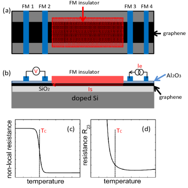
Figure 4: (color online). (a) and (b) are schematic diagrams for the proposed device. (a) is the top view and (b) is the side view. (c) and (d) schematically show the non-local resistance and the resistance $R_{23}$ versus the temperature, respectively.

Recently, graphene, a single-layer hexagonal lattice of carbon atoms, has been successfully fabricated.ref1a ; ref1b ; ref3 ; ref4 The unique structure of graphene leads to many peculiar properties, e.g., the relativistic-like quasi-particles spectrum.ref3 ; ref4 For graphene, the charge carriers are usually spin-unpolarized. However, if graphene is growing on a ferromagnetic (FM) materialref5 ; ref6 ; ref7 or is under an external magnetic fielda2ref1 , a spin split $M$ can be induced. Then the carriers are spin-polarized and the Dirac points with different spins are split. When the Fermi level lies in between the spin-resolved Dirac points (see Fig. 4(b)), the spin-up carriers are electron-like while the spin-down ones are hole-like. These positive and negative carriers attract and form e-h pairs that are stable against the e-h recombination due to the Coulomb interaction. This is because the filled electron-like states are now below the hole-like states, as shown in Fig. 4(b), unlike in conventional exciton systems in semiconductors (Fig. 4(a)) where the electron states are above the hole states. If a carrier jumps from the electron-like state to the hole-like one, the total energy of the system rises. This prevents the e-h recombination and means the e-h pairs in FM graphene is stable and can exist indefinitely in princeple. Therefore, this e-h pair gas can condense. In this work, we show that this condensate is a SSC and the spin current is dissipationless. We derive the London-type equations of the super-spin-current and find an electric ‘Meissner effect’ against the spatial variation of an electric field.

We consider an interacting electron system in graphene with the Hamiltonian $H=H_{0}+U_{C}$ where $H_{0}$ is the free Dirac fermion Hamiltonian and $U_{C}$ the electron-electron (e-e) Coulomb interaction:

$$H_{0} = \sum\limits_{{\bf k},\sigma}\Psi^{\dagger}_{{\bf k}\sigma}\left(\begin{array}[]{ll}-\sigma M&v_{F}(k_{x}-ik_{y})\\ v_{F}(k_{x}+ik_{y})&-\sigma M\end{array}\right)\Psi_{{\bf k}\sigma},$$ (3)

$$U_{C} = \sum\limits_{s,s^{\prime};i,j;\sigma,\sigma^{\prime}}U^{ss^{\prime}}_{ij}n^{s}_{i\sigma}n^{s^{\prime}}_{j\sigma^{\prime}},$$ (4)

where $\Psi_{{\bf k}\sigma}=(a_{{\bf k}\sigma},b_{{\bf k}\sigma})^{T}$, $s_{{\bf k}\sigma}$ $(s=a,b)$ are the Fourier components of the electron annihilation operators $s_{i\sigma}$ at sites $i$ for the sublattices $s$, and $n^{s}_{i\sigma}=s^{\dagger}_{i\sigma}s_{i\sigma}$ are the local electron number operators. ${\bf k}=(k_{x},k_{y})$ is the momentum, $\sigma=(\uparrow,\downarrow)$ represents the spin, $M$ is the FM exchange split energy, $U^{ss^{\prime}}_{ij}$ is the e-e Coulomb potential, and $v_{F}=3ta_{0}/2$ with the nearest hopping energy $t$ and the carbon-carbon distance $a_{0}$. Here we have ignored the valley degree of freedom, because the two valleys are degenerate and the inter-valley coupling is normally very weak due to the two valleys being well separated in k-space. Hereafter we also set the Fermi energy $E_{F}$ at zero. By taking a unitary transformation: $a_{{\bf k}\sigma}=\sum_{\tau}\tau c^{*}\alpha_{{\bf k}\tau\sigma}$ and $b_{{\bf k}\sigma}=\sum_{\tau}c\alpha_{{\bf k}\tau\sigma}$ with the pseudo spin index $\tau=\pm$, $c=e^{i\theta/2}/\sqrt{2}$ and $\theta=\tan^{-1}(k_{y}/k_{x})$, the free Hamiltonian $H_{0}$ can be diagonalized $H_{0}=\sum_{{\bf k},\tau,\sigma}\epsilon_{\tau\sigma}\alpha_{{\bf k}\tau\sigma}\alpha^{\dagger}_{{\bf k}\tau\sigma}$, where $\epsilon_{\tau\sigma}=-\sigma M+\tau v_{F}k$ are four energy bands (see the blue curves in Fig.1d) because the spin-degeneracy is lifted now. While $E_{F}=0$, $\epsilon_{-\uparrow}$ and $\epsilon_{+\downarrow}$ are high-energy bands. In the following, we focus on the low energy part and only two bands $\epsilon_{+\uparrow}$ and $\epsilon_{-\downarrow}$ are involved. Here the band $\epsilon_{+\uparrow}$ is electron-like, while the band $\epsilon_{-\downarrow}$ is hole-like and the annihilation operator $\alpha_{{\bf k}-\downarrow}$ also means to create a spin-up hole. Thus, we define operators $\alpha_{{\bf k}e\uparrow}=\alpha_{{\bf k}+\uparrow}$ and $\alpha^{\dagger}_{{\bf k}h\uparrow}=\alpha_{{\bf k}-\downarrow}$. The Hamiltonian $H_{0}$ can then be written as:

$$H_{0} = \sum\limits_{\bf k}(\alpha^{\dagger}_{{\bf k}e\uparrow},\alpha_{{\bf k}h\uparrow})\left(\begin{array}[]{ll}\epsilon_{+\uparrow}&0\\ 0&\epsilon_{-\downarrow}\end{array}\right)\left(\begin{array}[]{l}\alpha_{{\bf k}e\uparrow}\\ \alpha^{\dagger}_{{\bf k}h\uparrow}\end{array}\right).$$ (9)

For the e-e interaction $U_{C}$, we also focus on the two low-energy bands which are given by the terms $\alpha^{\dagger}_{{\bf k}-{\bf q},e\uparrow}\alpha_{{\bf k}e\uparrow}\alpha_{{\bf k}^{\prime}+{\bf q},h\uparrow}\alpha^{\dagger}_{{\bf k}^{\prime}h\uparrow}$. Furthermore, we keep only the terms whose momenta satisfy ${\bf k}-{\bf q}={\bf k}^{\prime}$, giving rise to the zero momentum e-h pair that is energetically favorable. Under these approximations, the interaction $U_{C}$ reduces to the attraction between electrons and holes

$$U_{C}=-\sum\limits_{{\bf k},{\bf k}^{\prime}}U_{{\bf k}{\bf k}^{\prime}}\alpha^{\dagger}_{{\bf k}^{\prime}e\uparrow}\alpha^{\dagger}_{{\bf k}^{\prime}h\uparrow}\alpha_{{\bf k}h\uparrow}\alpha_{{\bf k}e\uparrow},$$ (10)

where $U_{{\bf k}{\bf k}^{\prime}}=(U_{{\bf k}{\bf k}^{\prime}}^{ab}e^{i(\theta^{\prime}-\theta)}+U_{{\bf k}^{\prime}{\bf k}}^{ab}e^{i(\theta-\theta^{\prime})}+U_{{\bf k}{\bf k}^{\prime}}^{aa}+U_{{\bf k}{\bf k}^{\prime}}^{bb})/4$ with $U_{{\bf k}{\bf k}^{\prime}}^{ab}=\sum_{j}U^{ab}_{0j}e^{-i({\bf k}-{\bf k}^{\prime})\cdot({\bf r}_{j}+{\bf\delta})}$ and $U_{{\bf k}{\bf k}^{\prime}}^{ss}=\sum_{j}U^{ss}_{0j}e^{-i({\bf k}-{\bf k}^{\prime})\cdot{\bf r}_{j}}$ for the coordinate ${\bf r}_{j}$ of the site $j$ and the lattice spacing vector ${\bf\delta}$. $U_{\bf kk^{\prime}}$ is a large positive value at ${\bf k}={\bf k^{\prime}}$ and it gradually and oscillatorily decays to zero with increase of $|{\bf k}-{\bf k^{\prime}}|$. As discussed before, this attractive interaction does not induce the e-h recombination while it binds the electrons and holes into pairs. The mean field approximation of Eq. (10) reads

$$U_{C}\approx\sum_{\bf k}\Delta_{\bf k}\alpha^{\dagger}_{{\bf k}e\uparrow}\alpha^{\dagger}_{{\bf k}h\uparrow}+\sum_{\bf k}\Delta_{\bf k}^{*}\alpha_{{\bf k}h\uparrow}\alpha_{{\bf k}e\uparrow}$$

with the e-h pair condensation order parameter $\Delta_{\bf k}\equiv$$-\sum_{{\bf k}^{\prime}}U_{{\bf k}^{\prime}{\bf k}}\langle\alpha_{{\bf k}^{\prime}h\uparrow}\alpha_{{\bf k}^{\prime}e\uparrow}\rangle$.

Comparing with the spin singlet Cooper pair with charge $2e$, this e-h pair is of spin $\hbar$ and charge neutral. The total mean field Hamiltonian then is given by

$$H_{MF}=\sum\limits_{\bf k}(\alpha^{\dagger}_{{\bf k}e\uparrow},\alpha_{{\bf k}h\uparrow})\left(\begin{array}[]{ll}\epsilon_{+\uparrow}&\Delta_{\bf k}\\ \Delta_{\bf k}^{*}&\epsilon_{-\downarrow}\end{array}\right)\left(\begin{array}[]{l}\alpha_{{\bf k}e\uparrow}\\ \alpha^{\dagger}_{{\bf k}h\uparrow}\end{array}\right).$$ (15)

The energy spectrum for the mean field Hamiltonian $H_{MF}$ is shown in Fig. 4(d). An energy gap with the magnitude of $|\Delta_{\bf k}|$ is opened. When an electron and a hole combine into an e-h pair, the energy of the system is reduced by $2|\Delta_{\bf k}|$. This means the condensed state of the e-h pairs is more stable than the unpaired one. Thus, the ground state of FM graphene is a neutral superfluid with spin $\hbar$ per pair, namely, a SSC state. The spin current can dissipationlessly flow in the SSC and its spin resistance is zero.

The energy gap $\Delta$ can be estimated as follows. By using the definition $\Delta_{\bf k}\equiv-\sum_{{\bf k}^{\prime}}U_{{\bf k}^{\prime}{\bf k}}\langle\alpha_{{\bf k}^{\prime}h\uparrow}\alpha_{{\bf k}^{\prime}e\uparrow}\rangle$ and the Hamiltonian $H_{MF}$, one has the self-consistent equation:

$$\Delta_{\bf k}=\sum\limits_{{\bf k}^{\prime}}(U_{{\bf k}{\bf k}^{\prime}}\Delta_{{\bf k}^{\prime}}/2A)\{f(-A)-f(A)\},$$ (16)

where $f(A)=1/[\exp(A/k_{B}T)+1]$, $A=\sqrt{(M-k^{\prime})^{2}+\Delta_{{\bf k}^{\prime}}}$ and $T$ is the temperature. At zero temperature and assuming $U_{{\bf k}{\bf k}^{\prime}}=U\theta(k_{D}-|{\bf k}-{\bf k^{\prime}}|)$ with the cut-off momentum $k_{D}$, the self-consistent equation (16) reduces to $1=(U/2)\sum_{\bf k}\theta(k_{D}-k)/\sqrt{(M-k)^{2}+\Delta^{2}}=\frac{\sqrt{3}U}{3t^{2}}\int_{0}^{\epsilon_{D}}d\epsilon_{k}\frac{2\pi\epsilon_{k}}{\sqrt{(M-\epsilon_{k})^{2}+\Delta^{2}}}$, where $\epsilon_{D}=v_{F}k_{D}$. Numerically, we solve the self-consistent equation by using the e-e interaction $U_{C}$ with the nearest neighbor cut-off. The gaps vary as the cut-off $\epsilon_{D}$ for a fixed $M$ or as the FM split energy $M$ for a fixed $\epsilon_{D}$ are shown in Fig. 4(e) and (f), respectively. We see that the gap $\Delta$ grows faster than an exponential function with increase of $\epsilon_{D}$. When $M=5meV$ and $\epsilon_{D}=0.18t$,ref5 ; ref6 one gets $\Delta\approx 3$meV. This yields the critical temperature $T_{C}$ of the transition from the normal state to the SSC at about $30K$. Similar to the case in a superconductor, in the presence of weak impurities, $T_{C}$ is slightly reduced but the SSC phase can still exists if $T<T_{C}$, except in the case when the impurity strength is larger than $\Delta$ and its density is higher than $1/\xi^{2}$ with $\xi$ being the coherence length $\xi=\hbar v_{F}/\Delta$.

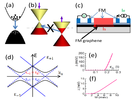
Figure 1: (color online). The schematic diagrams: (a) the band structure for the conventional exciton system; (b) for FM graphene; and (c) for the proposed four-terminal device to measure the SSC state. (d) The schematic energy bands of FM graphene for free electrons (blue curves) and for the e-h pair condensate (black curves). (e) The gap $\Delta$ vs. $\epsilon_{D}$ at the FM magnetic moment $M=5meV$ and (f) The gap vs. $M$ at $\epsilon_{D}=0.18t$.

Meissner effect is the criterion that a superconductor differs from a perfect metal: The magnetic field can not enter the bulk of a superconductor.meiss This phenomenon can be described by the London equations.london Is there a Meissner-like effect for the SSC? Consider a SSC with the superfluid carrier density $n_{s}$ in an electric field ${\bf E}$ and a magnetic field ${\bf B}$. A magnetic force ${\bf F}=({\bf m}\cdot\nabla){\bf B}$ acts on these spin carriers. Here ${\bf m}=(4\pi g\mu_{B}/h){\bf s}$ is the magnetic moment of a carrier; $\mu_{B}$ is the Bohr magneton and $g$ is the Lande factor. This force accelerates the carrier by Newton’s second law ${\bf F}=m^{*}d{\bf v}/dt$ for a carrier with the velocity ${\bf v}$ and the effective mass $m^{*}$. The spin current density $\mathbbm{J}_{s}=n_{s}{\bf v}{\bf s}$ is thus a tensor. The time derivative of this super-spin-current density $\mathbbm{J}_{s}$ is then given by

$$d\mathbbm{J}_{s}/dt=a(\mathbf{s}\cdot\nabla)\mathbf{B}\mathbf{s},$$ (17)

with the constant $a=4\pi g\mu_{B}n_{s}/hm^{*}$. Comparing with London’s first equation for the super-charge-current density:london $d{\bf J}/dt\propto{\bf E}$, the spatial variation of ${\bf B}$ along with the magnetic moment plays the role of an external field accelerating the spin carriers.

When an electric field ${\bf E}$ applies, by acting $({\bf s}\cdot\nabla)$ on two sides of the Maxwell equations$\nabla\times{\bf B}=\mu_{0}\epsilon_{0}\partial{\bf E}/\partial t$ and using Eq.(17), we obtain $\frac{\partial}{\partial t}[\nabla\times\mathbb{J}_{s}]=\frac{\partial}{\partial t}[\mu_{0}\epsilon_{0}a({\bf s}\cdot\nabla){\bf E}{\bf s}]$. Integrating over the time $t$, one has the equation for $\mathbb{J}_{s}$

$$\nabla\times\mathbb{J}_{s}=\mu_{0}\epsilon_{0}a({\bf s}\cdot\nabla){\bf E}{\bf s},$$ (18)

where the integral constant is taken to be zero because of the requirement of thermodynamic equilibrium. Instead of the magnetic field in London’s second equation for the superconductor,london the ‘external field’ here is the spatial variation of the electric field ${\bf E}$ along with the magnetic moment.

Eqs. (17) and (18) for $\mathbb{J}_{s}$ play roles similar to the London equations in superconductor.london For example, if the system is in the steady state, $d\mathbb{J}_{s}/dt=a({\bf s}\cdot\nabla){\bf B}{\bf s}=0$ implies that the variation $({\bf s}\cdot\nabla){\bf B}$ of the magnetic field along the direction of the FM magnetic moment ${\bf m}$ must be zero because of the zero spin resistance. On the other hand, Eq.(18) means the variation of the electric field, $({\bf s}\cdot\nabla){\bf E}$, is zero in bulk of the SSC. This is an electric ‘Meissner effect’ in the SSC against a spatial variation of an electric field.

We now give an example of this electric Meissner effect. Consider a positive charge $Q$ at the origin and an infinite FM graphene in the $x$-$y$ plane at $z=Z$ as shown in Fig. 2(a). The charge $Q$ generates an electric field ${\bf E}$ in FM graphene plane. This electric field will induce a super-spin-current in graphene against the spatial variation of ${\bf E}$. Assuming that the magnetic moment ${\bf m}$ (i.e., ${\bf s}$) is in the $z$-direction, then $({\bf s}\cdot\nabla)E_{z}=\partial_{z}E_{z}=\frac{Q}{4\pi\epsilon_{0}}\frac{r^{2}-2z^{2}}{(z^{2}+r^{2})^{5/2}}$ with $r^{2}=x^{2}+y^{2}$. Solving Eq.(18), one has the induced super-spin-current density $J_{s}=-\frac{\mu_{0}aQ}{4\pi}\frac{r}{(Z^{2}+r^{2})^{3/2}}$. This $J_{s}$ flows along the tangential direction (see Fig.2(a)) and its spin points to the $z$-direction. On the other hand, as a usual spin current,ref9 the super-spin-current density $J_{s}$ can generate an electric field ${\bf E}^{i}$ in space which is the same as that generated by the electric dipole moment $\vec{p}_{e}\propto(-\frac{r}{(Z^{2}+r^{2})^{3/2}},0,0)$ or the equivalent charge $Q_{i}=-\nabla\cdot\vec{p}_{e}\propto\frac{2Z^{2}-r^{2}}{(Z^{2}+r^{2})^{5/2}}$. In Fig.2(b), we plot the radial distributions in graphene for the variation $\partial_{z}E_{z}$ of the electric field of the original charge $Q$, the induced super spin current density $J_{s}$, and the equivalent charge $Q_{i}$ (i.e. the spatial variation $\partial_{z}E^{i}_{z}$). For $r<\sqrt{2}Z$ ($r>\sqrt{2}Z$) with $\partial_{z}E_{z}$ being negative (positive), the spatial variation $\partial_{z}E^{i}_{z}$ of the electric field ${\bf E}^{i}$ induced by the super-spin-current is positive (negative). As a result, $\partial_{z}E^{i}_{z}$ counteracts the variation $\partial_{z}E_{z}$ and then causes the variation of the total electric field in the SSC to vanish.

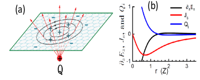
Figure 2: (color online). (a) The schematic diagram for the device consisting of a positive charge $Q$ and FM graphene. (b) The variation $\partial_{z}E_{z}$ ($Q/4\pi\epsilon_{0}$) of the electric field, the induced super-spin-current $J_{s}$ ($\mu_{0}aQ/8\pi$), and the equivalent charge $Q_{i}$ (i.e. $\partial_{z}E_{z}^{i}$) versus the radial distance $r$.

Josephson effect is another highlight of superconductivity and has wide applications.jose We now investigate the similar effect for this SSC by considering a device consisting of two SSCs which are weakly coupled by a normal conductor, i.e., a SSC/normal conductor/SSC junction (see Fig. 3(a)). We can explicitly show the existence of the super-spin-current in this device in equilibrium. The weakly coupled junction is described by the Hamiltonian $H=\sum_{\beta(\beta=L,R)}H_{\beta}+H_{c}+H_{T}$, where

$$H_{\beta} = \sum\limits_{\bf k}(\alpha^{\dagger}_{\beta{\bf k}e\uparrow},\alpha_{\beta{\bf k}h\uparrow})\left(\begin{array}[]{ll}\epsilon_{+\uparrow}&\Delta_{\beta{\bf k}}\\ \Delta_{\beta{\bf k}}^{*}&\epsilon_{-\downarrow}\end{array}\right)\left(\begin{array}[]{l}\alpha_{\beta{\bf k}e\uparrow}\\ \alpha^{\dagger}_{\beta{\bf k}h\uparrow}\end{array}\right),$$ (23)

$$H_{c} = \sum\limits_{\sigma}(\epsilon_{d}+\sigma M_{d})c^{\dagger}_{\sigma}c_{\sigma},$$

$$H_{T} = \sum\limits_{\beta,{\bf k}}\left[t_{\beta}\alpha^{\dagger}_{\beta{\bf k}+\uparrow}c_{\uparrow}+t_{\beta}\alpha^{\dagger}_{\beta{\bf k}-\downarrow}c_{\downarrow}+H.c.\right].$$

Namely, $H_{L/R}$, $H_{c}$, and $H_{T}$ are the Hamiltonians of the left/right SSC, the normal conductor, and the tunnelings between them, respectively. The order parameters $\Delta_{L/R{\bf k}}=\Delta e^{i\phi_{L/R}}$, where the SSC phases $\phi_{L/R}$ are assumed to be independent of the momentum ${\bf k}$. We consider a phase difference $\Delta\phi\equiv\phi_{L}-\phi_{R}$ between the left and right SSCs, which origins from a spin current flowing through the junction under the drive of an external device or from a variation of an external electric field thread the ring junction device. The normal conductor is described by a level (or a quantum dot) with the spin index $\sigma$ and spin-split energy $M_{d}$.

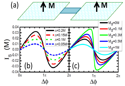
Figure 3: (color online). (a) The schematic diagram of the weakly coupled SSC-normal conductor-SSC junction. (b) The spin current $I_{s}$ vs. the phase difference $\Delta\phi$ for different $\Delta$ and $M_{d}=0$. (c) The $I_{s}$-$\Delta\phi$ curves for different $m_{d}$ and $\Delta=0.1M$. Here $\epsilon_{d}=0$ and $\Gamma\equiv 2\pi t^{2}_{\beta}\rho_{k}=0.1M$; $\rho_{k}$ is the density of state of FM graphene in momentum space.

The spin-dependent particle current $I_{\beta\sigma}$ with the spin $\sigma$ from the $\beta$ SSC to the central normal conductor can be calculated by the following equation,ref8 $I_{\beta\sigma}=Re(2t^{*}_{\beta}/\hbar)\int\frac{d\epsilon}{2\pi}G^{<}_{\beta\sigma,\sigma}(\epsilon)$, where the lesser Green function $G^{<}_{\beta\sigma,\sigma}(\epsilon)$ is the Fourier transformation of $G^{<}_{\beta\sigma,\sigma}(t)\equiv i\langle c^{\dagger}_{\sigma}(0)\alpha_{\beta{\bf k}\pm\sigma}(t)\rangle$. This Green function $G^{<}_{\beta\sigma,\sigma}(\epsilon)$ can be calculated by using the Dyson equation and so is the particle current $I_{\beta\sigma}$.ref8 Therefore, one can obtain the spin current $I_{s}=(I_{R\uparrow}-I_{R\downarrow})\hbar/2$ and the charge current $I_{e}=(I_{R\uparrow}+I_{R\downarrow})e$. The charge current $I_{e}$ is identically zero because the e-h pairs are charge neutral. The spin current $I_{s}$ versus $\Delta\phi$ in the equilibrium with zero bias and zero spin bias is calculated and shown in Fig. 3. There is a super-spin-current flowing through the junction that resembles the Josephson tunneling in a conventional superconductor junction. While Fig. 3(b) exhibits the $I_{s}$-$\Delta\phi$ curves for different values of the gap $\Delta$ with $m_{d}=0$, Fig. 3(c) shows $I_{s}$ can also be observed in non-zero $M_{d}$ as long as $\Delta\neq 0$ and $\Delta\phi\neq 0,\pi$.

In conclusion, a SSC state as well as the electric ‘Meissner effect’ and spin-current Josephson effect are predicted in FM graphene. For detection of the SSC, one can measure the zero spin resistance or super spin current. Based on the experiment in Ref.ref1b , here we propose a four-terminal device (as shown in Fig.1c) which can be used to measure the non-local resistance and then confirm the SSC state.sm A non-local resistance measurement means that a current is applied to the two right electrodes and the bias is measured on the two left electrodes.ref1b In this device, the non-local resistance is induced by a pure spin current flowing from right side through FM graphene (SSC) to left side.ref1b Once FM graphene turns into the SSC state by lowering temperature $T<T_{c}$, the spin current will flow with no dissipation, leading to a sharp increase of the non-local resistance (see the Fig.1c in the supplemental material). Due to the zero spin resistance effect in SSC, this sharp increase can be observed even in a macroscopic SSC device.

Acknowledgments: This work was financially supported by NSF-China under Grants Nos. 10734110, 10974015, 11074174, and 10874191, China-973 program and US-DOE under Grants No. DE-FG02- 04ER46124.

Supplementary information:

In this supplementary material we discuss how to detect the spin superconductor state. In the following we first suggest five measurable physical quantities or methods, and then follow up by proposing an experimental setup.

1) When the system enters the spin superconductor state, an energy gap opens up (see Fig.1d in the paper). This energy gap can be measured by ARPES or STM. When the temperature $T$ is lower (or higher) than the critical temperature $T_{C}$, the gap emerges (or disappears).

2) Because of the opening of an energy gap and the spin superconductor state does not carry charge current, the resistance sharply increases when the FM graphene enters from the normal metal state to the spin superconductor state. This sharp increase in resistance can be experimentally tested.

Notice that the measurements 1) and 2) are commonly done. These measurements demonstrate the opening of an gap and give strong hint that the sample may enter into the spin superconductor.

3) The zero spin resistance is a main characteristic for the spin superconductor. Due to the zero spin resistance, the spin current can flow without any dissipation even for a macroscopic sample. At the end of the supplementary material we propose a four-terminal device and in this device one can show zero spin resistance by measuring a non-local resistance.

4) In the Meissner effect for spin superconductor, an electric field applied to the spin superconductor can induce the super spin current on the surface of the sample. This induced super spin current can generate an electric field ${\bf E}^{i}$ that against the variation of the external electric field. Here the induced electric field ${\bf E}^{i}$ is equivalent to that generated by a certain surface charge distribution. In this case, the induced electric field and the equivalent surface charge distribution are the measurable quantities. For the example of Fig.2 in the paper, the equivalent surface charge $Q_{i}$ is proportional to $\frac{n_{s}}{m^{*}}\frac{2Z^{2}-r^{2}}{(Z^{2}+r^{2})^{5/2}}$, this value is quite large due to the smallness of the effective mass $m^{*}$ in graphene. But the equivalent surface charge $Q_{i}$ is still finite even if $m^{*}=0$, since once it reaches the complete shielding and the variation of the total electric field is zero, no more super spin current and charge are induced. By considering the complete shielding case, the inducing surface charge $Q_{i}=\frac{2Z^{2}-r^{2}}{(Z^{2}+r^{2})^{5/2}}\frac{Qd}{4\pi}$, where $d\approx 0.1nm$ is the thickness of graphene. Let us estimate the value of $Q_{i}$. We assume that the distance $Z$ between the external charge $Q$ and the plane of graphene is $10nm$ and $Q$ is a basic charge. The inducing surface charge $Q_{i}$ is about $10^{13}m^{-2}$ at the position $r=0$. This surface charge is quite large and should be measurable.

5) The super spin current in the the spin superconductor state or in the spin-current Josephson effect is also a measurable physical quantity. For example, it can be directly measured by observing the second-harmonic generation of the Faraday rotation as done in reference, Nature physics 6, 875 (2010).

In addition, many indirect methods have successfully measured the spin current, e.g., by probing the spin accumulation (Science 306, 1910(2004)), or probing the bias due to the inverse spin Hall effect (Nature 442, 176(2006)), or probing the bias through a quantum point contact (Nature 458, 868(2009), etc. These methods can also be used in our system. Let us imagine a spin current flowing into the spin superconductor (FM graphene) from one terminal, this spin current can flow through the spin superconductor with no dissipation and flows out to another terminal. Then we can measure the (usual) spin current at the outside through the aforementioned methods.

Notice that it is not necessary to do all of the aforementioned measurements. In fact, if one can take a measurement either in 3), 4), or 5), it establishes the presence of the spin superconductor.

Now let us suggest an experiment setup and propose a detailed experimental process.

Based on the device in the paper of Nature 488, 571 (2007), we propose a four-terminal device consisting of a graphene ribbon coupled by four FM electrodes and a long FM strip, as shown in the Fig.1(a) and (b). Except for the long FM strip (the red region), the device is what used in the paper of Nature 488, 571 (2007). So this device can be realized by the present technology. The ideal case is that the long red strip is a FM insulator which directly couples to the graphene without the $Al_{2}O_{3}$ layer. But even if this is hard to achieve, it is also fine for the red region being a FM metal. Graphene in the red region has a FM exchange splitting, and it is normal FM graphene at high temperature and turns to the spin superconductor at low temperature. Now we can qualitatively analyze the measurement results if the spin superconductor is realized. To simplify the analysis, we only consider the magnetic moments in all FM electrodes and strip are in the same direction.

Here we measure the non-local resistance as in the experimental paper of Nature 488, 571 (2007). In this measurement, a current is applied to two right electrodes (electrodes 3 and 4) and the bias is measured on two left electrodes (electrodes 1 and 2). When a current is applied between electrodes 3 and 4, it injects a pure spin current into graphene. This pure spin current flows from the electrode 3 through FM graphene (spin superconductor) to the left side (as shown in the Fig.1(b)). Then it induces the bias between the electrodes 1 and 2. When FM graphene is in the normal FM metal phase, it has a finite spin resistance. In this case, the spin current gradually decays along its transport direction, so the bias and the non-local resistance $R_{12,34}$ are small. Denoting $L_{ij}$ the distances between the electrode $i$ and $j$ and assuming $L_{12}$ and $L_{34}$ are much longer than the spin relaxation length $\lambda$ of the graphene in the normal state, the non-local resistance $R_{12,34}$ can be obtained analytically (see Nature 416, 713(2002); Nature 442, 176(2006); etc): $R^{normal}_{12,34}=\frac{1}{2}P^{2}\frac{\lambda}{\sigma_{G}W}e^{-L_{23}/\lambda}$, where $W$ is the width of the graphene ribbon, $P$ the spin polarization of the FM electrode, and $\sigma_{G}$ the conductivity of normal FM graphene. On the other hand, when FM graphene is in the spin superconductor phase, the spin resistance is zero and the spin current can flow through it with no dissipation. In this case, the non-local resistance can be obtained as $R_{12,34}^{SSC}=\frac{1}{2}P^{2}\frac{\lambda}{\sigma_{G}W}e^{-(L_{23}-L_{SSC})/\lambda}=R^{normal}_{12,34}e^{L_{SSC}/\lambda}$, which are much larger than $R^{normal}_{12,34}$. Therefore, a sharp increase in the non-local resistance can be observed (see the Fig.1(c)) when FM graphene turns from the normal metal phase to the spin superconductor phase as temperature is lowered. Furthermore, the spin resistance in the spin superconductor is always zero regardless of the length of the spin-superconductor device, so the non-local resistance is independent of the length of spin superconductor system and the sharp increase in non-local resistance can be observed even in a macroscopic spin superconductor device. Experimentally, one can also observe the relation between the non-local resistance and the sample length to confirm the zero spin resistance.

In addition, if the long red strip is a FM insulator, a sharp increase can also be observed in the resistance $R_{23}$ between electrodes 2 and 3 (see the Fig.1(d)), as discussed in point 2).

Finally, we emphasize that the main body of the proposed device as well the pure spin current injected into graphene have been realized in an experiment (see Nature 488, 571 (2007), etc). So the proposed method is experimentally feasible.

References

- (1) H. K. Onnes, Leiden Comm. 122b, 122c (1911); for a text book, see D. Shoenberg, Superconducting, Cambridge University Press, 1952.
- (2) W. Meissner and R. Ochsenfeld, Naturwiss 21, 787 (1933).
- (3) B. D. Josephson, Phys. Lett. 1, 251 (1962).
- (4) S. A. Wolf, et al., Science 294, 1488 (2001); G. A. Prinz, Science 282, 1660 (1998).
- (5) J. Bardeen, L. N. Cooper and J. R. Schrieffer, Phys. Rev. 108, 1175 (1957).
- (6) E. Hanamura and H. Haug, Phys. Rep. 33, 209 (1977).
- (7) A review on the exciton can be found in S. A. Moskalenko and D. W. Snoke, Bose-Einstein condensation of excitons and biexcitons: and coherent nonlinear optics with excitons (Cambridge University Press, 2000).
- (8) B. Deveaud, et al., Phys. Rev. Lett. 67, 2355 (1991).
- (9) J. Feldmann, et al., Phys. Rev. Lett. 59, 2337 (1987).
- (10) R. Rapaport and G. Chen, J. Phys.: Condens. Matter 19, 295207 (2007).
- (11) K.S. Novoselov, et al., Science 306, 666 (2004); Nature (London) 438, 197 (2005); Y. Zhang, et al., Nature (London) 438, 201 (2005).
- (12) N. Tombros, et al., Nature (London) 448, 571 (2007).
- (13) C. W. J. Beenakker, Rev. Mod. Phys. 80, 1337 (2008); A. H. Castro Neto, et al., Rev. Mod. Phys. 81, 109 (2009).
- (14) N. M. R. Peres, Rev. Mod. Phys. 82, 2673 (2010).
- (15) H. Haugen et al., Phys. Rev. B 77, 115406 (2008); J. Linder et al., Phys. Rev. Lett. 100, 187004 (2008).
- (16) Q. Zhang et al., Phys. Rev. Lett. 101, 047005 (2008).
- (17) Y.-W. Son et al., Nature (London) 444, 347 (2006); E.-J. Kan et al., Appl. Phys. Lett. 91, 243116 (2007).
- (18) D. A. Abanin, et al., Science 332, 328 (2011).
- (19) F. London and H. London, Proc. Roy. Soc. A 155 , 71 (1935).
- (20) Q.-F. Sun, H. Guo, and J. Wang, Phys. Rev. B 69, 054409 (2004); Q.-F. Sun and X. C. Xie, Phys. Rev. B 72, 245305 (2005).
- (21) Q.-F. Sun, et al., Phys. Rev. B 61, 4754 (2000); Q.-F. Sun, J. Wang, and T.-H. Lin, Phys. Rev. B 59, 3831 (1999).
- (22) See supplementary material at http://link.aps.org/ supplemental/… .